| Issue |
A&A
Volume 597, January 2017
|
|
|---|---|---|
| Article Number | A127 | |
| Number of page(s) | 7 | |
| Section | The Sun | |
| DOI | https://doi.org/10.1051/0004-6361/201629656 | |
| Published online | 16 January 2017 | |
Lambda-shaped jets from a penumbral intrusion into a sunspot umbra: a possibility for magnetic reconnection⋆
1 Max-Planck-Institute für Sonnensystemforschung, Justus-von-Liebig-Weg 3, 37077 Göttingen, Germany
e-mail: This email address is being protected from spambots. You need JavaScript enabled to view it.
2 Bal Shiksha Sadan Society, 3-Ratakhet, Udaipur, Rajsathan, India
3 School of Space Research, Kyung Hee University, Yongin, 446-701 Gyeonggi Do, Korea
Received: 5 September 2016
Accepted: 24 October 2016
Abstract
We present the results of high resolution co-temporal and co-spatial photospheric and chromospheric observations of sunspot penumbral intrusions. The data were taken with the Swedish Solar Telescope (SST) on the Canary Islands. Time series of Ca II H images show a series of transient jets extending roughly 3000 km above a penumbral intrusion into the umbra. For most of the time series, jets were seen along the whole length of the intruding bright filament. Some of these jets develop a clear λ-shaped structure, with a small loop appearing at their footpoint and lasting for around a minute. In the framework of earlier studies, the observed transient λ shape of these jets suggests that they could be caused by magnetic reconnection between a curved arcade-like or flux rope-like field in the lower part of the penumbral intrusion and the more vertical umbral magnetic field forming a cusp-shaped structure above the penumbral intrusion.
Key words: Sun: chromosphere / Sun: photosphere / sunspots / Sun: granulation
Movies associated to Figs. 1 and 2 are available at http://www.aanda.org
© ESO, 2017
1. Introduction
High resolution observations have revealed that the chromosphere above sunspots is very dynamic at small scales. Jet-like phenomena observed above sunspot penumbrae (penumbral micro jets, Katsukawa et al. 2007) and above umbrae (umbral microjets, Bharti et al. 2013) in Ca II H are examples of such dynamic events. The penumbral micro jets are associated with transient brightenings and are observed at the boundaries of penumbral filaments. Their lifetime is approximately one minute, and the apparent speed projected on the image plane is about 100 km s-1. The length of these jets is approximately 1000–4000 km and their width is 400 km. Jurčák & Katsukawa (2008) found that they are aligned with the background magnetic field. Umbral microjets (Bharti et al. 2013) are likely also aligned with the background magnetic field. The typical length and width of umbral microjets is less than 1′′ and 0.̋3, respectively. They last around one minute. Reardon et al. (2013) found that penumbral micro jets show extended emission in the wings of spectral lines, thus giving a similar signature to Ellerman bombs (Ellerman 1917) outside the sunspot.
Other interesting dynamical phenomena in the sunspot chromosphere are brightenings and surge activity above light bridges (Roy 1973; Asai et al. 2001; Berger & Berdyugina 2003; Bharti et al. 2007; Louis et al. 2008, 2009; Shimizu et al. 2009; Shimizu 2011). In particular, Shimizu et al. (2009) and Shimizu (2011) clearly detected jet-like structures in light bridges. The observed bright plasma ejection was intermittent and recurrent for more than a day. The length of the bright ejections was reported to be 1500–3000 km, significantly less than the previously reported length, 10 000 km, of dark surges in Hα images by Roy (1973) and Asai et al. (2001). Shimizu et al. (2009) occasionally observed fan-shaped jets as well as a chain of ejections from one end the of the light bridge to the other. Fan-shaped jets emanating from a light bridge were also reported by Robustini et al. (2016), who concluded that they were driven by magnetic reconnection. Louis et al. (2008) reported arch-like structures above a light bridge and brightness enhancement along the light bridge. Bharti (2015) finds jets above a light bridge which reach up to coronal heights and the leading edge of jets are hotter in the transition region and corona. The jets show a coordinated behaviour – neighbouring jets move up and down together. Kleint & Sainz Dalda (2013) reported on brightenings above several unusual filamentary structures (umbral filaments) in a sunspot. Coronal images show end points of bright coronal loops end in these unusual filaments.
Sakai & Smith (2008) and Magara (2010) proposed models for penumbral microjets that build on magnetic reconnection taking place between more inclined magnetic field in penumbral filaments and a more vertical background field. A similar interpretation was proposed by Shimizu et al. (2009) for the (bidirectional) jets emanating from a light bridge.
Chromospheric jets and surges are also found outside active regions (Shibata et al. 2007). In particular, Shibata et al. (2007) found λ-shaped jets in the quiet chromosphere, which was interpreted to support the notion of reconnection between an emerging magnetic bipole and a preexisting uniform vertical field (Yokoyama & Shibata 1995). Such a loop configuration gives indirect evidence of small-scale reconnection in the solar atmosphere (Singh et al. 2012b; Yan et al. 2015). Particularly, Yan et al. (2015) found evidence for intermittent reconnection in a λ-shaped jet driven by loop advection and followed by an outflow that excites waves and jets. The authors interpret these phenomena respecively as the causes and consequences of reconnection. A detailed analysis of quiet sun jets is presented by Nishizuka et al. (2011). A study of anemone jets by Morita et al. (2010) suggests that jets are generated in the lower chromosphere. On the other hand, a multiwavelength study of a jet shows simultaneous appearance in the lower and upper atmosphere (Nishizuka et al. 2008). The appearance of jets in the atmosphere depends on the size of the bipole (Shibata et al. 2007).
The present study is based on the high resolution G-continuum, Ca II H and FeI 6302 Å observations taken with the Swedish Solar Telescope (SST) to detect λ-shaped jets above a penumbral intrusion into the umbra and possible mechanism for jets occurrence. This paper is organized as follows: in Sect. 2 we present the observations, in Sect. 3 we describe the λ-shaped jets and their association with the underlying photospheric umbral features, we then present our conclusions in Sect. 4.
2. Observations
The observations were carried out in various wavelength bands at the Swedish Solar Telescope (Scharmer et al. 2003), La Palma, Canary Islands on 2006 August 13. The sunspot belonged to the active region NOAA 10904 and positioned at the heliocentric angle θ = 40.15° (μ = 0.76). The sunspot was located at x = −556″ and y = −254″ on the solar disk.
The sunlight was divided into blue and red channels. In the blue beam, various interference filters were used to obtain images in the G band (4305 Å), G continuum (4363 Å), Ca II H (3968.5 Å) line core, and in the ling wing (0.06 Å away from line centre). The image scale in the blue beam corresponded to 0.041′′/pixel.
The red beam was fed to the Solar Optical Universal Polarimeter (SOUP, see Title & Rosenberg 1981) filter to scan the FeI 6302.5 Å line at six wavelength positions. The width of the filter was 75 mÅ. Full Stokes polarimetry was performed to measure the magnetic field vector at each pixel of the field of view. In addition, continuum (broad band) images at 6302 Å were recorded. The plate scale in the red beam corresponded to 0. 065′′/pixel. More details on the data acquisition and reconstruction are described in Hirzberger et al. (2009). Measurement of instrumental polarization effects of the SST optical setup was done by inserting calibration optics, consisting of a rotating polarizer and a quarter wave plate into the beam. A code developed by Selbing (2005) was used to determine the demodulation matrix (see Hirzberger et al. 2009, for more details.)
Speckle interferometric techniques (see, Hirzberger et al. 2009) were used to reconstructed the G-continuum, the Ca II H core and Ca II H wing time series and SOUP polarization data. In addition, the HeLIx inversion code (Lagg et al. 2004) was used to invert the Stokes vector data assuming a simple one-component-plus-straylight Milne-Eddington atmosphere. The obtained magnetic parameters were transformed to the local coordinate system and a code developed by Georgoulis (2005) was used to resolve the 180° ambiguity.
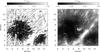 |
Fig. 1 Left panel: contrast-enhanced G-continuum image of the inner part of the observed sunspot at 9:11:31 UT. The arrow labelled “DC” points towards the disk centre. Right panel: cotemporal and cospatial contrast-enhanced Ca II H line core image. Locations labelled A, B and C in the left panel indicate penumbral intrusions where jet-like events are seen (see Movie 1 for more details). White boxes outline the field-of-view of events discussed in more details in the text. Enlargement of this box is shown in Fig. 2 and in the movies available online. The FOV is rotated by 90° clockwise so that the jets point upward. |
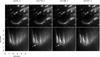 |
Fig. 2 Evolution of the jets and λ-shaped jets above penumbral intrusion C. Upper row: G-continuum images; lower row: simultaneous and cospatial images in the Ca II H line core. The plotted scene corresponds to the white squares in Fig. 1. Time Δt = 0 corresponds to 9:11:12 UT (see Movie 2 for more details). The white arrow indicates footpoint of a λ-shaped jet. |
3. Analysis and results
Contrast enhanced co-temporal and co-spatial images of the sunspot in the G continuum and in the Ca II H line core are displayed in Fig. 1. A broad light bridge (LB), a larger and a smaller umbrae is visible in both the images. In the G-continuum image both the umbrae show peripheral umbral dots and several dark patches (nuclei). However, in the larger umbra, central umbral dots and many penumbral intrusions are also recognised (Bharti et al. 2013). These intrusions are also visible with lower contrast in the Ca II H core image. Several jet-like transient bright structures are visible above penumbral filaments (penumbral microjets, cf. Katsukawa et al. 2007), LB (Shimizu et al. 2009; Shimizu 2011) and penumbral intrusions in the Ca II H core image (best seen in Movie 1, available online).
Occasionally bright jets similar to penumbral microjets are visible above penumbral intrusions A and B as can be gleaned from Movie 1. Around 9:11 UT we see the jets above intrusion B have a longer lifetime and a larger width than jets above intrusion A. Most striking is penumbral intrusion C, however. There, jets are both brighter and more extended than those from the other intrusions and occur without interruption over the entire observing span of approximately 47 min. The jets above the intrusion follow the orientation of the nearby penumbral microjets. In the following, we concentrate on the activity above penumbral intrusion C.
In the beginning, at 8:28:27 UT the jets occur only along the tip of this penumbral intrusion. Later on jets appear somewhat closer to the umbral-penumbral boundary. The jets’ length and brightness is higher around the tip of the filament. Around 9:02:01 UT a bunch of jets appears near the umbral-penumbral boundary with comparable length and brightness as around the tip of the filament. This strong jet activity then rapidly migrates along the intrusion into the umbra. Apart from migration, neighbouring jets also merge with each other. Such migration and merging of jets has been also reported above a light bridge in the transition region by Bharti (2015).
In Fig. 2, from 9:11:12 UT on, one can clearly see λ-shaped jets (the identification of these structures as “jets” is based on the comparison with similarly shaped features in the literature, e.g. Shibata et al. 2007). These are jets coming out of the tops of (small) loops whose footpoints lie in or next to the penumbral intrusion. Later, after 9:12:28 UT, again only elongated jets are visible in subsequent frames, although a weak λ-like structure is still discernible.
In the G-continuum images the penumbral intrusion shows a dynamical behaviour reminiscent of twisting motions and migrations of bright grains (see online Movie 2). A clear association of bright penumbral grain migration towards the umbra and the jets is visible around the tip of the penumbral intrusion from 8:42:23 UT to 8:45:52 UT. Similarly, from 9:11:12 UT onwards (i.e. starting with the appearance of λ-shaped jets), migration of bright penumbral grains towards the umbra in G-continuum images close to the footpoints of λ-shaped jets can be recognised.
We applied an intensity threshold (cf. Bharti et al. 2013, for more details) to determine various parameters of the jets. The projected lengths of jets are found to be 1700–3000 km. The λ-shaped jets belong to the shorter ones with lengths of 1700–1900 km. The separation between the footpoints of λ-shaped jet is 450–600 km and the loop at the bottom of the λ structure reaches a height of around 600 km above the loop base. These jets have shorter lengths than penumbral microjets (Katsukawa et al. 2007) but longer lengths than umbral microjets (Bharti et al. 2013). The lifetime of these jets (2–3 min) is comparable with penumbral microjets (Katsukawa et al. 2007) and umbral microjets (Bharti et al. 2013) as well as with jets reported in the umbra by Yurchyshyn et al. (2014).
Panel a of Fig. 3 displays the continuum intensity (broad band at 6302 Å) at 8:44:31 UT. The penumbral intrusion appears similar to that in the G-continuum (see Movie 2), but, due to the somewhat lower spatial resolution and contrast (caused by the longer wavelength), the fine structures are less clear.
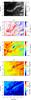 |
Fig. 3 Continuum image and plasma parameters from inversions of the Stokes profiles at around 6302 Å. a) Continuum at 6302 Å; b) line-of-site velocity; c) vertical component of the magnetic vector; d) inclination of magnetic vector (an inclination of 0 means a magnetic vector pointing vertically upward); e) azimuth. The overplotted contours outline the umbral-penumbral boundary in the continuum images. |
The line-of-sight velocity is depicted in panel b (positive velocity: blue shifted). The part of the intrusion close to the penumbra-umbra boundary shows upflows, similar to the ones typical of the inner penumbra, while the part away from the penumbra-umbra boundary shows upflows in the section towards disk centre and downflows away from disk centre. From x = 1.5′′ towards the tip of the intrusion only downflows are visible. The magnetic field strength is plotted in panel c. It is weaker in the intrusion compared to the surroundings, but always above 1 kG (in the mid-photosphere), again similar to filaments embedded in the penumbra. From panel d we infer that the field in the intrusion is more transverse, where the direction perpendicular to the solar surface refers to zero degrees. Interestingly, there is an opposite polarity patch, around x = 2.7′′ and y = 1.8′′, at the edge of the intrusion, close to the penumbra-umbra boundary. The azimuth (panel e) also shows about 90° rotation compared to the rest of the field surrounding the opposite polarity patch. The positive y axis is taken to correspond to a field azimuth of zero. The arrows overplotted on the intensity image in Fig. 4 show the horizontal field.
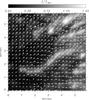 |
Fig. 4 Vectors showing the horizontal magnetic field structure overplotted on an intensity image. |
We note that there may be smaller amounts of opposite polarity flux also along other parts of the filament hidden by the dominant umbral field. Although we observe patches of opposite polarity, we are aware of the fact that with six wavelength points and highly redshifted profiles, this interpretation is not straightforward. Figure 5 shows observed and fitted profiles for an opposite polarity pixel. The pixel displays a highly redshifted Stokes I profile. The Stokes V profile has a peculiar shape; it looks like a superposition of two Stokes signals. Most likely one of the two components results from the strongly redshifted component, the other one, possibly, stems from the surrounding (straylight). If we look at the two components of the fit of this pixel one sees what HeLIx+ is trying to do: since the Stokes I profile does not match well with Stokes V it uses the straylight component (non-magnetic, blue) to fit Stokes I. The magnetic component gets a huge splitting in order to somehow match Q, U and V. With only six WL points, a much more complex interpretation is very difficult. The possibility of mis-interpreting the signal is quite high. The fit could definitely be improved by assuming two magnetic components, but with only 6 WL points such a fit cannot be done reliably. Since there are observational hints (Tiwari et al. 2013; Esteban Pozuelo et al. 2015) and well-established results from simulations (Rempel 2012) for the existence of opposite polarity field at the edges of penumbral filaments as well as in light bridges (Bharti et al. 2007; Lagg et al. 2014; Louis et al. 2014) the observed opposite polarity patches might be real. The presence of jets beyond the opposite polarity patch support this notion.
The left panel of Fig. 6 displays a Ca II H wing image of the penumbral intrusion at 08:44:55 UT. The umbral-penumbral boundary, and the penumbral intrusion as visible in the continuum image (6302 Å), are marked by white contours. The orange contour outlines the opposite polarity patch. In the Ca II H wing image the penumbral intrusion shows a filamentary structure with a central dark lane along its whole length. In continuum radiation, formed somewhat deeper than the line wing, the intrusion is much narrower and only the bright part adjacent to the central dark lane toward disk centre is clearly visible.
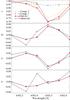 |
Fig. 5 Observed and fitted profiles for an opposite polarity pixel. Comp. 1 = the magnetic component of the ME-type atmosphere (blue) and Comp. 2 = the non-magnetic component of the ME-type atmosphere (usually the straylight contribution) (orange). Helix+ = sum of Comp. 1 + Comp. 2 (red) and fitted = the same as Helix+. |
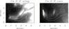 |
Fig. 6 Left: Ca II H wing image. An intensity threshold has been chosen to highlight the penumbral intrusion. Right: Ca II H core image. The white contours correspond to a continuum (6302 Å) threshold, the orange contour outlines the opposite polarity patch. All images were recorded around 08:44:55 UT. |
The other part, on the limbward side of the central dark lane, is hardly seen. We note that the sunspot is located away from the disc centre at θ = 40.15°, and the intrusion corresponds to an elevated structure (Lites et al. 2004) due to the raised optical depth unity level (Cheung et al. 2010). It is unclear if this 3D structure of the iso-τ surface is responsible for the difference in visibility and structure of the intrusion at different wavelengths. The velocities may also give an indication why the intrusion looks so different in the lower photosphere than in the middle and upper photosphere. The weak upflow in the disc centre side (i.e. in the continuum intrusion) and the strong downflows in the part close to the limb (visible only in the Ca wing) can be described as in Fig. 7. We propose that these flows have different physical causes: firstly, convection, with upflows on the disc centre side of the arcade and downflows on the other side. These convective flows heat the gas in the lower photosphere, but only at the location of the upflows, producing a narrow intrusion in lower photosphere. Secondly, in the upper photosphere and the chromosphere the intrusion is heated more by the reconnection, which accelerates the gas in both directions and thus brightens both parts of the intrusion located at the footpoints of the emerging arcade. The fact that the reconnection takes place closer to the limbward footpoint of the arcade may explain why the intrusion is brighter in Ca wing on the limbward side at many places. Due to increasing gas density with depth, the reconnection does not affect the lower photosphere. The width of the penumbral intrusion in the 6302 Å continuum images is 400–550 km, which is comparable to, but somewhat narrower than the footpoint separation of the λ-shaped jets in the Ca II H line core images (see Fig. 2). The width of the intrusion, as seen in the wing of Ca II H, is sufficient, however, to easily host both legs of the λ-shaped jets. The right panel of Fig. 6 depicts a Ca II H line core image with overplotted contours of the continuum (6302 Å) and the opposite polarity patch as in the left panel. At x = 2.7′′ and y = 1.8′′, a jet can be seen which seems to emerge directly from the opposite polarity. Close inspection of Movie 1 shows that the location of this jet activity corresponds to x = 8.5′′ and y = 6′′ in Ca II H that peaked at 08:44:55 UT. It is evident from Figs. 3 and 4 that there is also a downflow and opposite polarity patch surrounding x = 2.7′′ and y = 1.8′′. This location corresponds to the footpoints of the jets seen in Ca II H line core. Louis et al. (2014) found small-scale jets above light bridges in Ca II H line core images from Hinode (SOT) observations which are associated with localized patches of opposite polarity in the photosphere. The jets are triangular-shaped and exhibit a spike-like structure. The width of the filter used in the present study is narrower (1.1 Å) than the one used in Hinode (SOT/BFI). In addition, the spatial resolution of the present observations is nearly a factor of two higher, which might enable us to unravel the sub-structure (λ-shape) of the jets.
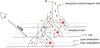 |
Fig. 7 Schematic picture of λ-shaped jets produced by magnetic reconnection between an emerging magnetic arcade along the penumbral intrusion and the pre-existing background umbral magnetic field. Thick arrows (brown) represent plasma accelerated by the reconnection, thin arrows indicate convective flows. The red stars mark the location of reconnection. |
4. Discussion and conclusion
We have for the first time clearly detected λ-shaped jets in a sunspot. These lie above a penumbral intrusion into the umbra. With a length of 1800 km they are at the small end of the quiet-sun λ-shaped jets (lengths of 2000–5000 km) reported by Shibata et al. (2007), based on Hinode/SOT Ca II H observations. This shape of a jet is considered to be a signal of reconnection between the loop connecting an emerging magnetic bipole and preexisting more vertical field (Yokoyama & Shibata 1995; Shibata et al. 1992, 2007). Robustini et al. (2016) also argue for magnetic reconnection as the driver of jets above a sunspot light-bridge. In our case a whole arcade of emerging flux is required, as we see jets all along the penumbral intrusion (or partial light bridge), although not all of them display a λ-type structure, possibly due to overlap between jets or insufficient spatial resolution. As can be deduced from the Movie 2, the group of jets to which the λ-shaped jets belong moves rapidly along the penumbral intrusion, starting at the umbral-penumbral boundary and ending at the tip of the intrusion. This implies an emerging arcade and suggests that the arcade first started to emerge near the umbra-penumbra boundary and later towards the tip of the intrusion. This notion is supported by the fact that we also see a migration of bright penumbral grains (in the G-continuum) toward the tip of the intrusion and close to the λ-shaped jets. Instead of an arcade, a rising and heavily twisted flux rope (and possibly rotating) could also be the cause the jets, or a strong elongated convective upwelling, carrying opposite polarity magnetic flux to its edges. Singh et al. (2012a) found systematic motions of λ-shaped jets outside a sunspot in Ca II H observations from Hinode in terms of migration from one end of the footpoint to the other end of an arcade that, finally, leads to a merging of jets similar to the merging of jets in the penumbral intrusion presented here. Such a morphology is illustrative of the emergence of twisted flux rope (see Fig. 4 of Singh et al. 2012a). The presence of the λ-shaped loops, however, requires a relatively ordered loop-like field, as illustrated in Fig. 7. This scenario is reproduced by a rising arcade of loops connected with convective upwelling. The convective upflow heats the gas in the lower photosphere thus loops connected with convective upwelling brightens the disk side penumbral intrusion in the continuum. The appearance of the bright λ-shaped loop in the upper photosphere is due to the heating caused by the reconnection, which accelerates the gas in both directions, filling both the loop with hot and bright gas as well as the jet above it.
Magara (2010) performed a magnetohydrodynamic simulation to explain penumbral microjets. In his model a strongly twisted flux rope (penumbral filament) is placed within the more vertical background field (umbral field). Magnetic reconnection takes place on the side of the flux rope with field lines having opposite polarity to the background field. Bharti et al. (2010a) found reverse polarities at edges of larger UDs, in the simulations of Schüssler & Vögler (2006), caused by strong convective downflows. The presence of opposite polarity along the lateral edges of penumbral filaments has been reported recently by Ruiz Cobo & Asensio Remos (2013), Scharmer et al. (2013), Tiwari et al. (2013) and Esteban Pozuelo et al. (2015). These opposite polarities are thought to be caused by convective downflows (Joshi et al. 2011; Scharmer et al. 2011). The observed up and downflows pattern, their correlation with lower photospheric brightness (bright upflows, dark downflows) opposite polarity and (possibly to a lesser extent) apparent twisting motions in the penumbral intrusion similar to penumbral filaments (Ichimoto et al. 2007; Zakharov et al. 2008; Bharti et al. 2010b, 2012) suggests that the intrusion is of convective nature similar to penumbral filaments, umbral dots and light bridges (Cheung et al. 2010). This supports the reconnection scenario of Magara (2010), although the full structure of the magnetic field may be different from what he proposed to produce a jet-like structure (see Tiwari et al. 2013). The approximate alignment of penumbral microjets with the background field found by Jurčák & Katsukawa (2008) was explained by Nakamura et al. (2012) as caused by reconnection between a weaker more horizontal and a stronger background field. Shimizu et al. (2009) proposed a model to interpret plasma ejections above an LB. In their model the current-carrying and highly twisted LB field is trapped below a cusp-shaped magnetic structure formed by the background field. This geometry is then proposed to lead to reconnection on the side of the LB at which the field is of opposite polarity to the umbral field. In a laboratory experiment Nishizuka et al. (2012) succeeded in producing jets that are qualitatively similar to penumbral jets as a result of magnetic reconnection in a roughly similar magnetic configuration. The general magnetic configuration presented by Magara (2010) and Shimizu et al. (2009) is in general agreement with our findings for the penumbral intrusion. However, different sources of the magnetic flux forming the arcade are possible. It may be an emerging arcade of loops along the intrusion, or an emerging or twisting flux rope. Finally, fields twisted and dragged down by magnetoconvection are also candidates. Since the λ jets are seen in chromospheric radiation and the loop at the base of the jet is around 600 km high, we expect that the reconnection is taking place in the upper photosphere.
Online material
Movie of Fig. 1 Access Supplementary Material
Movie of Fig. 2 Access Supplementary Material
Acknowledgments
Dr. Andreas Lagg is kindly acknowledged for help with inversions. The Swedish 1-m Solar telescope is operated on the island of La Palma by the Institute for Solar Physics of the Royal Swedish Academy of sciences in the Spanish Observatorio del Roque de los Muchachos of the Instituto de Astrofísica de Canarias. This work has been partly supported by the BKZI plus program through the NRF funded by the Korean Ministry of Education.
References
- Asai, A., Ishii, T., & Kurokawa, H. 2001, ApJ, 555, L65 [NASA ADS] [CrossRef] [Google Scholar]
- Berger, T. E., & Berdyugina, S. V. 2003, ApJ, 589, L117 [NASA ADS] [CrossRef] [Google Scholar]
- Bharti, L. 2015, MNRAS, 452, L16 [NASA ADS] [CrossRef] [Google Scholar]
- Bharti, L., Rimmele, T., Jain, R., Jaaffrey, S. N. A., & Smartt, R. N. 2007, MNRAS, 376, 1291 [Google Scholar]
- Bharti, L., Beek, B., & Schüssler, M. 2010a, A&A, 510, A12 [NASA ADS] [CrossRef] [EDP Sciences] [Google Scholar]
- Bharti, L., Solanki, S. K., & Hirzberger, J. 2010b, ApJ, 722, L194 [NASA ADS] [CrossRef] [Google Scholar]
- Bharti, L., Cameron, R. H., Rempel, M., Hirzberger, J., & Solanki, S. K. 2012, ApJ, 752, 128 [NASA ADS] [CrossRef] [Google Scholar]
- Bharti, L., Hirzberger, J., & Solanki, S. K. 2013, A&A, 552, L1 [NASA ADS] [CrossRef] [EDP Sciences] [Google Scholar]
- Cheung, M. C. M., Rempel, M., Title, A. M., & Schüssler, M. 2010, ApJ, 720, 233 [NASA ADS] [CrossRef] [Google Scholar]
- Ellerman, F. 1917, ApJ, 46, 298 [NASA ADS] [CrossRef] [Google Scholar]
- Esteban Pozuelo, S., Bellot Rubio, L. R., &de la Cruz Rodríguez, J. 2015, ApJ, 803, 93 [NASA ADS] [CrossRef] [Google Scholar]
- Georgoulis, M. K. 2005, ApJ, 629, L69 [NASA ADS] [CrossRef] [Google Scholar]
- Hirzberger, J., Riethmüller, T., Lagg, A., Solanki, S. K., & Kobel, P. 2009, A&A, 505, 771 [NASA ADS] [CrossRef] [EDP Sciences] [Google Scholar]
- Ichimoto, K., Suematsu, Y., Tsuneta, S., et al. 2007, Science, 318, 1597 [NASA ADS] [CrossRef] [PubMed] [Google Scholar]
- Joshi, J., Pietarila, A., Hirzberger, J., et al. 2011, ApJ, 734, L18 [NASA ADS] [CrossRef] [Google Scholar]
- Jurčák, J., & Katsukawa, Y. 2008, A&A, 488, L33 [NASA ADS] [CrossRef] [EDP Sciences] [Google Scholar]
- Katsukawa, Y., Berger, T. E., Ichimoto, K., et al. 2007, Science, 318, 1594 [NASA ADS] [CrossRef] [Google Scholar]
- Kleint, L., & Sainz Dalda, A. 2013, ApJ, 770, 74 [NASA ADS] [CrossRef] [Google Scholar]
- Lagg, A., Woch, J., Krupp, N., & Solanki, S. K. 2004, A&A, 414, 1109 [NASA ADS] [CrossRef] [EDP Sciences] [Google Scholar]
- Lites, B. W., Scharmer, G. B., Berger, T. E., & Title, A. M. 2004, Sol. Phy., 221, 65 [Google Scholar]
- Louis, R. E., Bayanna, A. R., Mathew, S. K., & Venkatakrishnan, P. 2008, Sol. Phys., 252, 43 [NASA ADS] [CrossRef] [Google Scholar]
- Louis, R. E., Bellot Rubio, L. R., Mathew, S. K., & Venkatakrishnan, P. 2009, ApJ, 704, L29 [NASA ADS] [CrossRef] [Google Scholar]
- Louis, R. E., Beck, C., & Ichimoto, K. 2014, A&A, 567, A96 [NASA ADS] [CrossRef] [EDP Sciences] [Google Scholar]
- Magara, T. 2010, ApJ, 715, L40 [NASA ADS] [CrossRef] [Google Scholar]
- Morita, S, Shibata, K., Ueno, S., et al. 2010, PASJ, 62, 901 [NASA ADS] [CrossRef] [Google Scholar]
- Nakamura, N., Shibata, K., & Isobe, H. 2012, ApJ, 761, 87 [NASA ADS] [CrossRef] [Google Scholar]
- Nishizuka, N., Shimizu, M., Nakamura, T., et al. 2008, ApJ, 683, L83 [NASA ADS] [CrossRef] [Google Scholar]
- Nishizuka, N., Nakamura, T., Kawate, T., Singh, K. P. A., & Shibata, K. 2011, ApJ, 731, 43 [NASA ADS] [CrossRef] [Google Scholar]
- Nishizuka, N., Hayashi, Y., Tanabe, H., et al. 2012, ApJ, 756, 152 [NASA ADS] [CrossRef] [Google Scholar]
- Reardon, K., Tritschler, A., & Katsukawa, Y. 2013, ApJ, 779, 143 [NASA ADS] [CrossRef] [Google Scholar]
- Rempel, M. 2012, ApJ, 750, 62 [NASA ADS] [CrossRef] [Google Scholar]
- Robustini, C., Leenaarts, J., de la Cruz Rodríguez, J., & Rouppe van der Voort, L. 2016, A&A, 590, A57 [NASA ADS] [CrossRef] [EDP Sciences] [Google Scholar]
- Roy, J. 1973, Sol. Phys., 28, 95 [NASA ADS] [CrossRef] [Google Scholar]
- Ruiz Cobo, B., & Asensio Ramos, A. 2013, A&A, 549, L4 [NASA ADS] [CrossRef] [EDP Sciences] [Google Scholar]
- Sakai, J. I., & Smith, P. D. 2008, ApJ, 687, L127 [NASA ADS] [CrossRef] [Google Scholar]
- Scharmer, G. B., Bjelksjo, K., Korhonen, T. K., Lindberg, B., & Petterson, B. 2003, Proc. SPIE, 4853, 341 [Google Scholar]
- Scharmer, G. B., Henriques, V. M. J., Kiselman, D., & de la Cruz Rodríguez, J. 2011, Science, 333, 316 [NASA ADS] [CrossRef] [Google Scholar]
- Scharmer, G. B., de la Cruz Rodriguez, J., Sütterlin, P., & Henriques, V. M. J. 2013, A&A, 553, A63 [NASA ADS] [CrossRef] [EDP Sciences] [Google Scholar]
- Schüssler, M., & Vögler, A. 2006, ApJ, 641, L73 [NASA ADS] [CrossRef] [Google Scholar]
- Selbing, J. 2005, Master Thesis, Stockholm Observatory [Google Scholar]
- Shibata, K., Ishido, Y., Acton, L., et al. 1992, PASJ, 44, 173 [Google Scholar]
- Shibata, K., Nakamura, T., Matsumoto, T., et al. 2007, Science, 318, 1591 [NASA ADS] [CrossRef] [Google Scholar]
- Shimizu, T. 2011, ApJ, 738, 83 [NASA ADS] [CrossRef] [Google Scholar]
- Shimizu, T., Katsukawa, Y., Kubo, M., et al. 2009, ApJ, 696, 66 [Google Scholar]
- Singh, K. A. P., Isobe, H., Nishida, K., & Shibata, K. 2012a, ApJ, 760, 28 [NASA ADS] [CrossRef] [Google Scholar]
- Singh, K. A. P., Isobe, H., Nishizuka, N., Nishida, K., & Shibata, K. 2012b, ApJ, 759, 33 [NASA ADS] [CrossRef] [Google Scholar]
- Title, A. M., & Rosenberg, W. J. 1981, Opt. Eng., 20, 815 [NASA ADS] [CrossRef] [Google Scholar]
- Tiwari, S. K., van Noort, M., Lagg, A., & Solanki, S. K. 2013, A&A, 557, A25 [NASA ADS] [CrossRef] [EDP Sciences] [Google Scholar]
- Yan, L., He, J., Xia, L., & Jiao, F. 2015, ApJ, 804, 69 [NASA ADS] [CrossRef] [Google Scholar]
- Yokoyama, T., & Shibata, K. 1995, Nature, 375, 42 [NASA ADS] [CrossRef] [Google Scholar]
- Yurchyshyn, V., Abramenko, V., Kosovichev, A., & Goode, P. 2014, ApJ, 787, 58 [NASA ADS] [CrossRef] [Google Scholar]
- Zakharov, V., Hirzberger, J., Riethmüller, T. L., Solanki, S. K., & Kobel, P. 2008, A&A, 488, L17 [NASA ADS] [CrossRef] [EDP Sciences] [Google Scholar]
All Figures
|
Fig. 1 Left panel: contrast-enhanced G-continuum image of the inner part of the observed sunspot at 9:11:31 UT. The arrow labelled “DC” points towards the disk centre. Right panel: cotemporal and cospatial contrast-enhanced Ca II H line core image. Locations labelled A, B and C in the left panel indicate penumbral intrusions where jet-like events are seen (see Movie 1 for more details). White boxes outline the field-of-view of events discussed in more details in the text. Enlargement of this box is shown in Fig. 2 and in the movies available online. The FOV is rotated by 90° clockwise so that the jets point upward. |
| In the text | |
|
Fig. 2 Evolution of the jets and λ-shaped jets above penumbral intrusion C. Upper row: G-continuum images; lower row: simultaneous and cospatial images in the Ca II H line core. The plotted scene corresponds to the white squares in Fig. 1. Time Δt = 0 corresponds to 9:11:12 UT (see Movie 2 for more details). The white arrow indicates footpoint of a λ-shaped jet. |
| In the text | |
|
Fig. 3 Continuum image and plasma parameters from inversions of the Stokes profiles at around 6302 Å. a) Continuum at 6302 Å; b) line-of-site velocity; c) vertical component of the magnetic vector; d) inclination of magnetic vector (an inclination of 0 means a magnetic vector pointing vertically upward); e) azimuth. The overplotted contours outline the umbral-penumbral boundary in the continuum images. |
| In the text | |
|
Fig. 4 Vectors showing the horizontal magnetic field structure overplotted on an intensity image. |
| In the text | |
|
Fig. 5 Observed and fitted profiles for an opposite polarity pixel. Comp. 1 = the magnetic component of the ME-type atmosphere (blue) and Comp. 2 = the non-magnetic component of the ME-type atmosphere (usually the straylight contribution) (orange). Helix+ = sum of Comp. 1 + Comp. 2 (red) and fitted = the same as Helix+. |
| In the text | |
|
Fig. 6 Left: Ca II H wing image. An intensity threshold has been chosen to highlight the penumbral intrusion. Right: Ca II H core image. The white contours correspond to a continuum (6302 Å) threshold, the orange contour outlines the opposite polarity patch. All images were recorded around 08:44:55 UT. |
| In the text | |
|
Fig. 7 Schematic picture of λ-shaped jets produced by magnetic reconnection between an emerging magnetic arcade along the penumbral intrusion and the pre-existing background umbral magnetic field. Thick arrows (brown) represent plasma accelerated by the reconnection, thin arrows indicate convective flows. The red stars mark the location of reconnection. |
| In the text | |
Current usage metrics show cumulative count of Article Views (full-text article views including HTML views, PDF and ePub downloads, according to the available data) and Abstracts Views on Vision4Press platform.
Data correspond to usage on the plateform after 2015. The current usage metrics is available 48-96 hours after online publication and is updated daily on week days.
Initial download of the metrics may take a while.