© ESO, 2016

1. Introduction

The magnetic activity of the Sun follows an 11-year cycle. At the time of minimum activity, the surface magnetic field is concentrated at the polar caps and presents a strongly dipolar configuration. As the cycle progresses, new magnetic flux erupts in the form of bipolar magnetic regions (BMRs). The preceding polarity (relative to the Sun’s sense of rotation) of the new BMRs tends to emerge closer to the equator (Joy’s law), and is of the same sign as the polar field in the same hemisphere at the immediately previous activity minimum (Hale’s law). The latitudinal separation of polarities favors the cross-equatorial transport of preceding polarity flux, which causes the gradual cancellation and eventual reversal of the polar fields. When the next activity minimum is reached, the global field is again nearly dipolar and reversed with respect to the previous activity minimum. The full magnetic cycle is therefore 22 yr long. These activity cycles show pronounced variability, both cycle to cycle and on longer time scales (for a review of the solar cycle, see Hathaway 2015).

It has been shown that the strength of the polar fields at activity minima strongly correlates with the amplitude of the subsequent cycle (see, for example, Schatten et al. 1978; Choudhuri 2008; Wang & Sheeley 2009; Muñoz-Jaramillo et al. 2013). This is supportive of the Babcock-Leighton model of solar dynamo, in which the polar fields at activity minima represent the poloidal field threading the Sun, from which the toroidal field of the next cycle is generated, rather than being a secondary manifestation of a dynamo mechanism operating below the surface (Cameron & Schüssler 2015). It follows that, in this framework, an activity-related feedback mechanism affecting the surface transport of magnetic flux could provide a means for saturating the dynamo by limiting the build-up of the polar fields (and therefore the regeneration of the poloidal field) and possibly also contribute to the observed variability of the cycle amplitude. One candidate for such a mechanism are the near-surface, converging flows towards active regions (Cameron & Schüssler 2012). These flows, first reported by Gizon et al. (2001), have magnitudes of ~50 m s^-1 and can extend up to 30° away from the center of the active region. The inflows are possibly driven by the temperature gradient arising from the enhanced radiative loss in areas of strongly concentrated magnetic field (Spruit 2003; Gizon & Rempel 2008).

The question of how these inflows affect the surface transport of magnetic flux and the build-up of the polar fields has been addressed in a number of works. Their main effect is the limitation of the latitudinal separation of the polarities of BMRs, which causes a reduction of the global dipole with respect to a no-inflows scenario (Jiang et al. 2010). This effect dominates in strong cycles, while in weaker cycles the inflows driven by low-latitude BMRs mainly enhance the cross-equatorial transport of magnetic flux, resulting in stronger polar fields. The inclusion of the inflows in surface flux transport simulations improves the correlations of the amplitude of the global dipole with the inferred open heliospheric flux in cycles 13 to 21 (Cameron & Schüssler 2012), but produces a weaker match with the observed butterfly diagram and dipole reversal times in cycles 23 and 24 (Yeates 2014).

All the studies cited above modelled the inflows as an axisymmetric perturbation of the meridional flow converging towards the activity belts. De Rosa & Schrijver (2006) included a more realistic model of inflows in their surface flux transport model, but the converging flows severely affected the dispersal of magnetic flux in their simulations, leading to unrealistic clumping of magnetic flux despite the diffusion by supergranules. In a recent work (Martin-Belda & Cameron 2016), we studied the impact of the inflows in the evolution of an isolated BMR, and showed that turbulent diffusion and differential rotation are sufficiently strong to counteract the converging flows, which decline quickly owing to flux cancellation. A probable reason for the discrepancy with the aforementioned study is the additional damping of the turbulent diffusivity inside active regions, which these authors included to match observations. We argued that the inflows alone can cause this effect.

In this work we continue studying the effect of the inflows on the surface transport of magnetic flux. Our main question is the impact that realistic, non axisymmetric inflows may have on the generation of the large-scale poloidal field. As mentioned above, this could provide a non-linear saturation mechanism for the global dynamo and contribute to the solar cycle variability. A second problem concerns whether our previous result on the dispersal of flux against converging flows holds in global simulations. To address these questions, we incorporated two non-axisymmetric parametrizations of the inflows in a surface flux transport model. The paper is structured as follows: we first introduce our model (Sect. 2); then, we examine a case with inflows whose strength and extension are compatible with observations (Sect. 3); next, we carry out a parameter study to test how these two magnitudes, as well as the activity level, may affect the build-up of the global magnetic dipole at activity minima (Sect. 4); finally, the results are summarized and briefly discussed (Sect. 5).

2. Surface flux transport model

2.1. Surface flux transport equation

The evolution of the magnetic field on the solar surface is governed by the radial component of the induction equation (DeVore et al. 1984): $\begin{array}{ccc}\frac{\mathit{\partial }{\mathit{B}}_{\mathit{r}}}{\mathit{\partial t}}& \mathrm{=}& \mathrm{-}\frac{\mathrm{1}}{{\mathit{R}}_{\mathrm{\odot }}\sin \mathit{\theta }}\left[\frac{\mathit{\partial }\mathrm{\left(}{\mathit{B}}_{\mathit{r}}{\mathit{u}}_{\mathit{\theta }}\sin \mathit{\theta }\mathrm{\right)}}{\mathit{\partial \theta }}\mathrm{+}\frac{\mathit{\partial }\mathrm{\left(}{\mathit{B}}_{\mathit{r}}{\mathit{u}}_{\mathit{\phi }}\mathrm{\right)}}{\mathit{\partial \phi }}\right]\\ & & \\ & & \mathrm{+}\mathit{S}\mathrm{\left(}\mathit{\theta ,\phi ,t}\mathrm{\right)}\mathit{,}\end{array}$(1)where φ and θ denote solar longitude and colatitude, respectively. The first term on the right hand side represents the advection of magnetic flux by the surface flows, which include differential rotation, meridional flow, and inflows towards active regions: $\begin{array}{ccc}& & {\mathit{u}}_{\mathit{\theta }}\mathrm{=}{\mathit{v}}_{\mathrm{m}}\mathrm{\left(}\mathit{\theta }\mathrm{\right)}\mathrm{+}{\mathit{w}}_{\mathit{\theta }}\mathrm{\left(}\mathit{\theta ,\phi }\mathrm{\right)}\\ & & {\mathit{u}}_{\mathit{\phi }}\mathrm{=}{\mathit{R}}_{\mathrm{\odot }}\sin \mathit{\theta }\hspace{0.17em}\mathrm{\Omega }\mathrm{\left(}\mathit{\theta }\mathrm{\right)}\mathrm{+}{\mathit{w}}_{\mathit{\phi }}\mathrm{\left(}\mathit{\theta ,\phi }\mathrm{\right)}\mathit{.}\end{array}$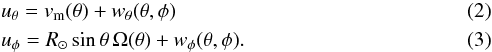Here, v_m is the velocity of the meridional flow, Ω(θ) is the angular velocity of the differential rotation and w_φ and w_θ are the components in spherical coordinates of the inflows.

We adopt the differential rotation profile from Snodgrass (1983): $\mathrm{\Omega }\mathrm{\left(}\mathit{\theta }\mathrm{\right)}\mathrm{=}\mathrm{13.38}\mathrm{-}\mathrm{2.30}{\cos }^{\mathrm{2}}\mathit{\theta }\mathrm{-}\mathrm{1.62}{\cos }^{\mathrm{4}}\mathit{\theta }{\mathrm{[}}^{\mathrm{◦}}\mathit{/}\mathrm{day}\mathrm{]}\mathit{.}$(4)Following van Ballegooijen et al. (1998), we model the meridional flow as ${\mathit{v}}_{\mathrm{m}}\mathrm{\left(}\mathit{\lambda }\mathrm{\right)}\mathrm{=}\{\begin{array}{c}\\ & \mathrm{if}\mathrm{\left|}\mathit{\lambda }\mathrm{\right|}\mathit{<}{\mathit{\lambda }}_{\mathrm{0}}\\ & \mathrm{if}\mathrm{\left|}\mathit{\lambda }\mathrm{\right|}\mathrm{\ge }{\mathit{\lambda }}_{\mathrm{0}}\mathit{,}\end{array}$(5)where λ denotes solar latitude and λ₀ = 75°.

The second term on the right hand side of Eq. (1)describes the flux dispersal by convective flows as a random walk/diffusion process (Leighton 1964). We choose η = 250 km²/ s, a value in agreement with observations (Schrijver & Martin 1990; Jafarzadeh et al. 2014) and consistent with the evolution of the large scale fields (Cameron et al. 2010).

The term S(θ,φ,t) describes the emergence of new active regions, and is described in detail in Baumann et al. (2004). The synthetic activity cycles in our simulations are 13 yr long, with a two-year overlap between cycles, so the time distance between consecutive cycle minima is 11 yr. The activity level (the number of new BMRs per day) is governed by a Gaussian function whose height peaks halfway into the cycle. At the beginning of the cycle, the BMRs emerge at a mean latitude of 40° with a standard deviation of 10°. These values decrease linearly and reach a mean latitude of 5° and a standard deviation of 5° at the end of the cycle. We do not consider active longitudes in this study, so the random distribution is uniform in φ. Following van Ballegooijen et al. (1998), we represent a BMR by two circular patches of opposite polarity. The magnetic field of each patch is given by: ${\mathit{B}}_{\mathit{r}}\mathrm{\left(}\mathit{\theta ,\phi }\mathrm{\right)}\mathrm{=}{\mathit{B}}_{\max }{\left(\frac{\mathit{\delta }}{{\mathit{\delta }}_{\mathrm{0}}}\right)}^{\mathrm{2}}\exp \begin{array}{c}\mathrm{⎧}\\ \mathrm{⎪}\\ \mathrm{⎪}\\ \mathrm{⎨}\\ \mathrm{⎪}\\ \mathrm{⎪}\\ \mathrm{⎩}\end{array}\mathrm{-}\frac{\mathrm{2}\mathrm{[}\mathrm{1}\mathrm{-}\cos {\mathit{\beta }}_{\mathrm{\pm }}\mathrm{(}\mathit{\theta ,\phi }\mathrm{\left)}\mathrm{\right]}}{{\mathit{\delta }}_{\mathrm{0}}^{\mathrm{2}}}\begin{array}{c}\mathrm{⎫}\\ \mathrm{⎪}\\ \mathrm{⎪}\\ \mathrm{⎬}\\ \mathrm{⎪}\\ \mathrm{⎪}\\ \mathrm{⎭}\end{array}\mathit{,}$(6)where β_± is the heliocentric angle between the center of the (±) polarity patch and the surface point (θ,φ); δ denotes the angular size of the BMR and δ₀ = 4°. The size of the BMRs follows a distribution n(δ) ∝ δ⁴. This distribution was derived by Schrijver & Harvey (1994) from observations for BMRs with sizes ranging from 3.5° to 10°. BMRs smaller than 3.5° cannot be well resolved in our simulations, so they are assumed to diffuse without interacting with the rest of the flux until they reach this size. The maximum field strength upon emergence, B_max, is adjusted so the total flux input per cycle is ~ 8.9 × 10²⁴ Mx (Schrijver & Harvey 1994).

2.2. Parametrization of the inflows

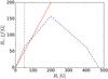Fig. 1 Br (orange line) and ξf (dashed, blue line) as a function of Br. The dashed vertical line indicates Br = 50 G.

We test two different models of inflows. The first one is based upon the parametrization of Cameron & Schüssler (2012), 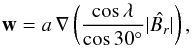${w}\mathrm{=}\mathit{a}\hspace{0.17em}\mathrm{\nabla }\left(\frac{\cos \mathit{\lambda }}{\cos {\mathrm{30}}^{\mathrm{◦}}}\mathrm{\left|}\widehat{{\mathit{B}}_{\mathit{r}}}\mathrm{\right|}\right)\mathit{,}$(7)where $\mathrm{\left|}\widehat{{\mathit{B}}_{\mathit{r}}}\mathrm{\right|}$ is the absolute value of the magnetic field smoothed with a Gaussian. Adjusting the full width at half maximum (FWHM) of the Gaussian allows us to control the extension of the inflows. We note that the gradient of the smoothed magnetic field generally decreases with increasing width of the Gaussian. Hence, for a fixed value of a, wider inflows are weaker. The factor cosλ/ cos30° is introduced to quench unrealistically strong poleward flows arising from the gradient of the polar fields. Figure 2 shows the inflows around an activity complex for our reference values a = 1.8 × 10⁸ m²/ G s and FWHM = 15°. The value of a is chosen so that the peak inflow velocity around an isolated BMR of size 10° is ~50 m/s, in agreement with observations. Hereafter we refer to this parametrization as the B-parametrization.

The second parametrization of the inflows is motivated by the results of Vögler (2005). The author’s radiative MHD simulations suggest that the relation between the average magnetic field in an active region and the integrated radiation flux is non-monotonic, peaking at about ~200 G. For stronger average fields, the formation of dark pores reduces the radiation output. This can effectively reduce the radiative cooling in active regions, and thus limit the strength of the inflows. We attempt to capture this effect by substituting B_r in Eq. (7)with the angle integrated radiation flux normalized to the quiet-Sun value (which we denote by f), taken from the left panel of Fig. 2 in Vögler (2005), 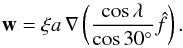${w}\mathrm{=}\mathit{\xi a}\hspace{0.17em}\mathrm{\nabla }\left(\frac{\cos \mathit{\lambda }}{\cos {\mathrm{30}}^{\mathrm{◦}}}\mathit{f̂}\right)\mathit{.}$(8)The prefactor ξ = 6.3 × 10⁴ was adjusted such that the peak inflow velocity around an isolated, 10°-sized BMR is ~50 m/s for our reference values of a and the FWHM. This parametrization is referred to as f-parametrization in the remainder of the paper. The f-parametrization produces weaker inflow velocities in regions of strong magnetic field. However, since the slope of f is steeper than the slope of B between 0 and 50 G (see Fig. 1), the contribution to the inflows of areas with fields lower than 50 G value to the inflows will be stronger than in the B-case.

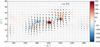Fig. 2 Model of inflows towards an activity complex formed by several emerged BMRs. The colour scale encodes the strength of the magnetic field Br in Gauss and saturates at 250 G. Red and blue indicate opposite polarities. The values of the parameters in Eq. (7)are a = 1.8 × 108 m2 G-1 s-1 and FWHM = 15°.

One of the problems we address in this paper is the suppression of magnetic flux dispersal in the presence of inflows found by De Rosa & Schrijver (2006). These authors parametrize the inflows in the following way: ${w}\mathrm{=}\mathit{a}\mathrm{\nabla }\mathrm{|}{\mathit{B}}_{\mathit{r}}{\mathrm{|}}^{\mathit{b}}\mathit{.}$(9)This parametrization (with b = 1) is the same as ours except for the geometric factor that is similar to the one introduced in Cameron & Schüssler (2012) to prevent strong inflows near the poles.

2.3. Numerical treatment

To integrate Eq. (1), we developed a surface flux transport code. The equation is expressed in terms of x = cosθ. We calculate the x-derivative in the advection term with a fourth-order centered finite differences scheme. The derivative in the φ direction is calculated in Fourier space. We use a fourth-order Runge-Kutta scheme to advance the advection terms in time. The diffusion term in the x-direction is treated with a Crank-Nicolson scheme. We treat the φ-diffusion term by computing the exact solution of the diffusion equation for the Fourier components of B_r.

We validated the code by reproducing the results for the reference case of the study by Baumann et al. (2004).

Calculating the inflows requires smoothing the absolute value of the magnetic field (or the normalized radiation flux, in the f-parametrization) with a Gaussian of given FWHM every time step. The result of this operation is identical to diffusing | B_r | (or f) with a given diffusion coefficient η_s for a time interval Δt′, related to the FWHM of the smoothing Gaussian through $\mathit{FWHM}\mathrm{=}\mathrm{4}\sqrt{\mathrm{\Delta }{\mathit{t}}^{\mathrm{\prime }}\hspace{0.17em}{\mathit{\eta }}_{\mathrm{s}}\hspace{0.17em}\ln \mathrm{2}}\mathit{.}$(10)We emphasize that the time t′ in Eq. (10)is different to the simulation time t. The diffusion of | B_r | or f is a mathematical resource that we employ to compute the inflows every time step, and is therefore unrelated to the diffusion term in Eq. (1), which describes the physical surface diffusion of B_r by the convective flows.

The numerical integration of the diffusion equation for | B_r | or f is performed in a number n of time steps that must be large enough for the implicit scheme to produce a reasonably accurate solution and avoid Gibbs oscillations, which lead to instabilities in the simulation. The number n should also be as small as possible to minimize the computational cost. We tested two different approaches to matching this compromise. The straightforward solution is to use time steps of equal size δt′ = Δt′/n. By a process of trial and error, we find that n = 50 satisfies the required conditions. The second approach relies on the fact that the time steps need to be shorter when the gradient of the function to diffuse is steeper. Since the steepest gradients are reduced as the diffusion progresses, taking time steps of increasing size enables us to reduce n. If we allow every time step be longer than the preceding one by a factor γ, then $\mathit{\delta }{\mathit{t}}^{\mathrm{\prime }}\mathrm{=}\frac{\mathrm{\Delta }{\mathit{t}}^{\mathrm{\prime }}}{\mathrm{1}\mathrm{+}\mathit{\gamma }\mathrm{+}{\mathit{\gamma }}^{\mathrm{2}}\mathrm{+}\mathit{...}\mathrm{+}{\mathit{\gamma }}^{\mathit{n}\mathrm{-}\mathrm{1}}}\mathrm{=}\frac{\mathrm{1}\mathrm{-}\mathit{\gamma }}{\mathrm{1}\mathrm{-}{\mathit{\gamma }}^{\mathit{n}}}\mathrm{\Delta }{\mathit{t}}^{\mathrm{\prime }}\mathit{,}$(11)where δt′ is now the size of the first step. We find that the combination γ = 1.7 and n = 8 satisfies the above requirements and leads to results that are consistent with the first approach.

Figure 2 shows an example of inflows towards an area of strong magnetic field.

3. Reference case

3.1. Setup

We first study the impact of the inflows on the amplitude of the polar fields for our reference values, a = 1.8 × 10⁸ m²/ G s and FWHM = 15°. We ran three sets of simulations: without inflows, with inflows, and with an axisymmetric perturbation of the meridional flow calculated as the azimuthal average of the inflows. The latter is done for comparison with Cameron & Schüssler (2012). While our treatment is not equivalent to the one in the cited study, the calibration factors ensure that the axisymmetric inflows in both studies have similar strengths. To reduce the statistical noise arising from the random positioning of the sources, we ran 20 realizations for each set of parameters. Each realization spans 55 years.

The initial configuration of the magnetic field is chosen such that the rate of poleward flux transport by the meridional flow and the rate of equatorward transport by turbulent diffusion are approximately equal, v_mB_r ≈ (η/R_⊙)∂B_r/∂θ, which corresponds to a situation of activity minimum (see van Ballegooijen et al. 1998). Combining this with Eq. (5)yields ${\mathit{B}}_{\mathit{r}}\mathrm{\left(}\mathit{\lambda }\mathrm{\right)}\mathrm{=}\{\begin{array}{c}\\ & \mathrm{if}\mathrm{\left|}\mathit{\lambda }\mathrm{\right|}\mathit{<}{\mathit{\lambda }}_{\mathrm{0}}\\ & \mathrm{if}\mathrm{\left|}\mathit{\lambda }\mathrm{\right|}\mathrm{\ge }{\mathit{\lambda }}_{\mathrm{0}}\mathit{,}\end{array}$(12)where a₀ = v_mR_⊙λ₀/θη. B₀ is chosen in each simulation by requiring that the strength of the polar fields at activity minima remains approximately constant from cycle to cycle.

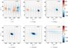Fig. 3 Time series showing the evolution of a long-standing, single-polarity magnetic flux clump. Time progresses from left to right and from top to bottom. The colour scale indicates the magnetic field strength in Gauss and saturates at 350 G. The arrows represent the strength and direction of the inflows.

3.2. Flux dispersal

Regarding the surface transport of magnetic flux, one of the main questions is how the magnetic flux contained in active regions that are surrounded by inflows spreads. De Rosa & Schrijver (2006) found that including the inflows in surface flux transport simulations led to a suppression of the flux dispersal by convective flows, resulting in the formation of magnetic flux clumps that are incompatible with observations. In Martin-Belda & Cameron (2016), we showed that, in the case of an isolated magnetic region, flux cancellation in the first days after emergence causes a decrease in the strength of the inflows, so that turbulent diffusion and the shearing caused by the differential rotation are sufficient to explain the flux dispersal. However, the interaction between neighbouring active regions can result in the formation of polarity-imbalanced magnetic patches. In such cases, flux cancellation no longer decreases the inflow strength. In our simulations, this leads to the occasional formation of highly concentrated, single-polarity flux clumps which can last for years. This is much longer than the typical decay time of active regions, which ranges from days to weeks (see, e.g., Schrijver & Zwaan 2008). By contrast, the flux clumping discussed in De Rosa & Schrijver (2006) possibly arises owing to the additional reduction of the diffusivity inside active regions that was included by these authors in their model. By reducing the diffusivity in active regions, these authors sought to account for the observed reduction of the flux dispersal in the core of active regions (Schrijver & Martin 1990). In Martin-Belda & Cameron (2016), we argued that the inflows alone would have a similar effect.

Figure 3 shows the formation and evolution of one such long-lasting polarity clump. The first panel shows an active region complex that consists of two large patches of magnetic flux, drawing strong inflows, and a BMR to the left of it. Some of the negative polarity of the BMR is attracted towards the active complex by the inflows, and cancels part of the complex’s positive flux. The positive patch of the BMR, further away from the complex, is less affected and diffuses away rapidly. This causes a flux imbalance in the complex (we emphasize that magnetic flux is still conserved globally), leading to the formation of the single-polarity feature (top-middle). The persistent inflows further concentrate its flux, until an approximate equilibrium between diffusion and the inflows is reached. As the patch is advected towards higher latitudes, the shear that is caused by the differential rotation, the partial cancellation with the polar field, and the artificial decrease of the inflow strength that is caused by the prefactor cosλ/ cos30° of our parametrization lead to the dispersal of the single-polarity patch.

The formation and evolution of single-polarity features in simulations using the f-parametrization is essentially parallel to the one described for the B-parametrization, but the magnetic field is substantially less concentrated. This is demonstrated in Fig. 4, which represents the peak magnetic field of the single-polarity patch as a function of time in both parametrizations. An initial concentration of the magnetic field takes place in approximately the first two months of evolution. This is followed by a dip, possibly caused by the assimilation of positive polarity flux from a decaying BMR, much in the same way the single-polarity feature formed by mainly assimilating one of the polarities of a BMR. A plateau phase follows, in which the average magnetic field of the single-polarity feature, which we may estimate as ~ B_r,max/ 2, is ~ 300 G in the B-parametrization case and ~ 150 G in the f-parametrization (although a slightly increasing trend can be seen in the B-parametrization case). This phase lasts slightly longer than a year, after which the feature begins to decay owing to the reasons stated above.

The lower concentration of magnetic flux in the long-standing clumps in the f-parametrization suggests that a less idealized parametrization of this mechanism may solve the clumping problem completely.

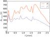Fig. 4 Maximum field strength of the single-polarity patch under discussion. The orange and dashed, blue lines correspond respectively to the B- and the f-parametrizations of the inflows.

3.3. Evolution of the axial dipole moment

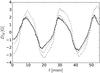Fig. 5 Evolution of the axial dipole moment in one realization with the B-parametrization of the inflows. The (dashed) green, (dotted) purple and black lines correspond to simulations without inflows, with azimuthally averaged inflows and with non-axisymmetric inflows, respectively. Otherwise, the setup of all three simulations is identical.

To evaluate the impact of the inflows on the reversal and regeneration of the large-scale poloidal field we study the evolution of the axial dipole moment of the surface field, which is defined as: ${\mathit{D}}_{\mathit{M}}\mathrm{=}\sqrt{\frac{\mathrm{3}}{\mathrm{4}\mathit{\pi }}}{\mathrm{\int }}_{\mathrm{0}}^{\mathrm{2}\mathit{\pi }}{\mathrm{\int }}_{\mathrm{0}}^{\mathit{\pi }}{\mathit{B}}_{\mathit{r}}\mathrm{\left(}\mathit{\phi ,\theta }\mathrm{\right)}\cos \mathit{\theta }\sin \mathit{\theta }\hspace{0.17em}\mathrm{d}\mathit{\theta }\mathrm{d}\mathit{\phi }\mathit{.}$(13)Figure 5 shows the evolution of the axial dipole moment in three simulations (without inflows, with azimuthally averaged inflows and with full inflows) using the B-parametrization of the inflows. The set of sources is identical in all three realizations. The dipole amplitude is larger in the run without inflows than in the runs with inflows and with azimuthally averaged inflows. In the case of non axisymmetric inflows, D_M is generally lower than in the case with averaged inflows, although values can occasionally be higher owing to statistical fluctuations. Averaging the peak values of the dipole moment over 20 realizations yields the following average axial dipole amplitudes: 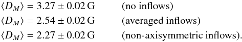$\begin{array}{ccc}\mathrm{⟨}{\mathit{D}}_{\mathit{M}}\mathrm{⟩}\mathrm{=}\mathrm{3.27}\mathrm{\pm }\mathrm{0.02}\hspace{0.17em}\mathrm{G}& & \mathrm{\left(}\mathrm{noinflows}\mathrm{\right)}\\ \mathrm{⟨}{\mathit{D}}_{\mathit{M}}\mathrm{⟩}\mathrm{=}\mathrm{2.54}\mathrm{\pm }\mathrm{0.02}\hspace{0.17em}\mathrm{G}& & \mathrm{\left(}\mathrm{averagedinflows}\mathrm{\right)}\\ \mathrm{⟨}{\mathit{D}}_{\mathit{M}}\mathrm{⟩}\mathrm{=}\mathrm{2.27}\mathrm{\pm }\mathrm{0.02}\hspace{0.17em}\mathrm{G}& & \mathrm{(}\mathrm{non}\mathrm{-}\mathrm{axisymmetricinflows}\mathrm{)}\mathrm{.}\end{array}$The amplitude of the axial dipole moment in the case with azimuthally averaged inflows is, on average, ~22% lower than in the case without inflows. In the case of non-axisymmetric inflows, the average amplitude is ~30% lower.

The average dipole peak strength obtained from the simulations using the f-parametrization is ~ 3% lower than in the B-case: $\begin{array}{ccc}\mathrm{⟨}{\mathit{D}}_{\mathit{M}}\mathrm{⟩}\mathrm{=}\mathrm{2.20}\mathrm{\pm }\mathrm{0.02}\hspace{0.17em}\mathrm{G}\mathrm{(}\mathrm{non}\mathrm{-}\mathrm{axisymmetric,f}\mathrm{-}\mathrm{parametrization}\mathrm{)}\mathrm{.}& & \end{array}$The slight difference is due to the stronger contribution of fields up to 50 G in this parametrization (see Sect. 2.2), which causes a greater restriction of the latitudinal separation of polarities than in the B-case.

The small difference between the average axial dipole moment in the B- and f-cases suggests that the occasional single-polarity clumps do not have a significant impact on the amplitude of the global dipole moment. This is because the single-polarity features occur only very occasionally, so the amount of flux that would have crossed the equator, had the feature been allowed to disperse, is much smaller than the total flux crossing the equator over the cycle. For this reason, we proceed by performing a parameter study of our inflow model using only the B-parametrization.

4. Parameter study

4.1. Inflow parameters

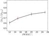Fig. 6 Average amplitude of the axial dipole moment (⟨ DM ⟩) relative to the no-inflows case (⟨ DM,0 ⟩) as a function of the FWHM. The red square symbol indicates the reference case. The error bars indicate a deviation of 1σ from the mean.

To understand the way the two parameters of our model influence the build-up of the axial dipole, we compared the strength of the dipole that results from simulations with and without inflows. The FWHM of the inflows was varied over the range 12° to 25°, while keeping a to its reference value of 1.8 × 10⁸ m² G^-1 s^-1. Similarly, a was varied from 2 × 10⁷ to 3 × 10⁸ m² G^-1 s^-1 with fixed FWHM = 15°. We ran 20 realizations for each combination of parameters.

Figure 6 shows the variation of the average dipole peak amplitude with the FWHM of the smoothing Gaussian. For all the values of the FWHM, the average amplitude of the axial dipole moment decreases relative to their no-inflows counterpart. This is due to the quenching of the contribution of the BMRs to the global dipole induced by the inflows, which is determined by the magnetic flux of the BMR and the latitudinal separation of the polarities (Martin-Belda & Cameron 2016). The inflows enhance the cancellation of opposite polarity flux and limit the latitudinal separation of the polarities, which results in a reduction of this contribution. With decreasing FWHM, the stronger and more localized inflows further enhance these effects, resulting in a larger reduction of the axial dipole moment. The axial dipole moment ratio varies from ~ 60% to ~ 80% in the range of FWHM under consideration.

Figure 7 shows the average peak amplitude of the axial dipole moment as a function of the multiplicative parameter a in Eqs. (7)and (8). For a = 2 × 10⁷ m² G^-1 s^-1, the average peak amplitude of the axial dipole is only slightly smaller than in the no-inflows case. Larger values of a render stronger inflows, and the amplitude of the dipole consequently decreases. For the strongest inflows that we considered (a = 3 × 10⁸ m² G^-1 s^-1), the amplitude of the axial dipole moment is ~ 50% weaker than in the case without inflows.

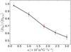Fig. 7 Average amplitude of the axial dipole moment (⟨ DM ⟩) relative to the no-inflows case (⟨ DM,0 ⟩) as a function of the multiplicative parameter a in Eq. (7). The red square symbol indicates the reference case. The error bars indicate a deviation of 1σ from the mean.

4.2. Activity level

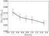Fig. 8 Average amplitude of the axial dipole moment (⟨ DM ⟩) relative to the corresponding no-inflows case (⟨ DM,0 ⟩) as a function of the cycle strength. The symbols indicate the chosen values for the activity level, relative to the activity of the reference case (indicated with the red square symbol). The error bars indicate a deviation of 1σ from the mean.

We ran simulations with an activity level, defined as the number of active regions per 11-yr cycle, ranging from 0.2 to 1.5 times that of the reference case. The dependence of the average peak amplitude of the axial dipole moment (relative to the no-inflows scenario) with activity is shown in Fig. 8. The ratio of dipole moments decreases with the activity level by about a 9% over the whole activity range. This is because, in strong cycles, owing to the larger number of active regions, the collectively driven inflows have a stronger impact on the latitudinal separation of the polarities of individual BMRs. This decrease in the relative amplitude of the axial dipole moment with activity implies that, in the Babcock-Leighton framework, the generation of the poloidal field is more efficient in weak cycles than in strong ones. This constitutes a non-linearity, which may saturate the dynamo and possibly contribute to the modulation of the solar magnetic cycle.

There is a second way inflows can affect the build-up of the axial dipole, namely, enhanced cross-equatorial transport of flux owing to inflows driven by low-latitude active regions. This effect is less pronounced in strong cycles than in weak ones, since the former peak earlier than the latter (Waldmeier rule) and, as a consequence, the inflows during the maxima of strong cycles are further away from the equator. Since all our simulations peak halfway into the cycle, and thus do not include the Waldmeier effect, the influence of the activity level on the build-up of the axial dipole may be even more pronounced than found here.

5. Conclusion

We used a surface flux transport code to study the role of near-surface, converging flows towards active regions on the surface transport of magnetic flux and the build-up of an axial dipole at cycle minima. The inflows have been proposed as one possible non-linear mechanism behind the saturation of the global dynamo in the Babcock-Leighton framework (Cameron & Schüssler 2012). We stress that other mechanisms, such as alpha-quenching (Ruediger & Kichatinov 1993) or cycle-dependent thermal perturbations of the overshoot region affecting the stability of the flux tubes and, as a consequence, the tilt angle of the emerging flux tubes (Işık 2015), have also been proposed. Here we concentrate on the inflows, but we do not mean to suggest that in this paper we exclude other possibilities.

We first studied the evolution of the surface flux in a case with inflows that have strengths and extensions similar to those observed on the Sun. In Martin-Belda & Cameron (2016), we found that the strength of the inflows driven by an isolated BMR decays owing to the cancellation of opposite-polarity flux over approximately the first 30 days of evolution. Differential rotation and turbulent diffusion are strong enough to ensure the flux dispersal. However, as seen in Sect. 3.2, interaction between neighbouring active regions can occasionally give rise to large single-polarity concentrations. In these cases, a mechanism other than flux cancellation may be required to weaken the inflows and allow for the dispersal of the single-polarity clump. One possibility is that the darkening caused by the formation of pores in areas of strong magnetic field leads to a reduction in the cooling beneath the active region, rendering the inflows weaker. We explored this possibility in our simulations and saw that, although the clumping persists, the magnetic field of these features is substantially lower than in the simulations where the effect of pore-darkening is not considered. This result suggests that this mechanism may be operating in the Sun, although less idealized models of inflows may be necessary to fully account for the clumping problem. In any case, the occasional occurrence of single-polarity clumps in the simulations does not have a significant impact on the amplitude of the global dipole.

We also performed a parameter study in which we varied the strength and extension of the inflows and the activity of the cycles. In general, inflows decrease the axial dipole moment at the end of the cycle. This is due to the relative decrease in latitudinal separation of the polarities of BMRs caused by the inflows. Stronger (weaker) inflows lead to larger (smaller) reductions of the axial dipole moment.

Our main finding is that inflows with characteristics that are similar to those observed can reduce the axial dipole moment at the end of the cycle by ~ 30% with respect to the case without inflows in cycles of moderate activity. This ratio varies by ~ 9% from very weak cycles to very strong cycles, which supports the notion of inflows being a potential non-linear mechanism capable of limiting the field amplification in a Babcock-Leighton dynamo and contributing to the modulation of the solar cycle.

Acknowledgments

We want to thank Manfred Schüssler for his valuable suggestions and his thorough revision of this manuscript. D.M.B. acknowledges postgraduate fellowship of the International Max Planck Research School on Physical Processes in the Solar System and Beyond. This work was carried out in the context of Deutsche Forschungsgemeinschaft SFB 963 “Astrophysical Flow Instabilities and Turbulence” (Project A16).

References

All Figures

	Fig. 1 Br (orange line) and ξf (dashed, blue line) as a function of Br. The dashed vertical line indicates Br = 50 G.
In the text

	Fig. 2 Model of inflows towards an activity complex formed by several emerged BMRs. The colour scale encodes the strength of the magnetic field Br in Gauss and saturates at 250 G. Red and blue indicate opposite polarities. The values of the parameters in Eq. (7)are a = 1.8 × 108 m2 G-1 s-1 and FWHM = 15°.
In the text

	Fig. 3 Time series showing the evolution of a long-standing, single-polarity magnetic flux clump. Time progresses from left to right and from top to bottom. The colour scale indicates the magnetic field strength in Gauss and saturates at 350 G. The arrows represent the strength and direction of the inflows.
In the text

	Fig. 4 Maximum field strength of the single-polarity patch under discussion. The orange and dashed, blue lines correspond respectively to the B- and the f-parametrizations of the inflows.
In the text

	Fig. 5 Evolution of the axial dipole moment in one realization with the B-parametrization of the inflows. The (dashed) green, (dotted) purple and black lines correspond to simulations without inflows, with azimuthally averaged inflows and with non-axisymmetric inflows, respectively. Otherwise, the setup of all three simulations is identical.
In the text

	Fig. 6 Average amplitude of the axial dipole moment (⟨ DM ⟩) relative to the no-inflows case (⟨ DM,0 ⟩) as a function of the FWHM. The red square symbol indicates the reference case. The error bars indicate a deviation of 1σ from the mean.
In the text

	Fig. 7 Average amplitude of the axial dipole moment (⟨ DM ⟩) relative to the no-inflows case (⟨ DM,0 ⟩) as a function of the multiplicative parameter a in Eq. (7). The red square symbol indicates the reference case. The error bars indicate a deviation of 1σ from the mean.
In the text

	Fig. 8 Average amplitude of the axial dipole moment (⟨ DM ⟩) relative to the corresponding no-inflows case (⟨ DM,0 ⟩) as a function of the cycle strength. The symbols indicate the chosen values for the activity level, relative to the activity of the reference case (indicated with the red square symbol). The error bars indicate a deviation of 1σ from the mean.
In the text

References

- Baumann, I., Schmitt, D., Schüssler, M., & Solanki, S. K. 2004, A&A, 426, 1075 [NASA ADS] [CrossRef] [EDP Sciences] [Google Scholar]
- Cameron, R., & Schüssler, M. 2012, A&A, 548 [Google Scholar]
- Cameron, R., & Schüssler, M. 2015, Science, 347, 1333 [NASA ADS] [CrossRef] [Google Scholar]
- Cameron, R., Jiang, J., Schmitt, D., & Schüssler, M. 2010, ApJ, 719, 264 [NASA ADS] [CrossRef] [Google Scholar]
- Choudhuri, A. R. 2008, J. Astrophys. Astron., 29, 41 [NASA ADS] [CrossRef] [Google Scholar]
- De Rosa, M., & Schrijver, C. 2006, in Proc. SOHO 18/GONG 2006/HELAS I, Beyond the spherical Sun, ESA SP, 624, 12 [NASA ADS] [Google Scholar]
- DeVore, C. R., Boris, J. P., & Sheeley, Jr., N. R. 1984, Sol. Phys., 92, 1 [Google Scholar]
- Gizon, L., & Rempel, M. 2008, Sol. Phys., 251, 241 [NASA ADS] [CrossRef] [Google Scholar]
- Gizon, L., Duvall, Jr., T. L., & Larsen, R. M. 2001, in Recent Insights into the Physics of the Sun and Heliosphere: Highlights from SOHO and Other Space Missions, eds. P. Brekke, B. Fleck, & J. B. Gurman, IAU Symp., 203, 189 [Google Scholar]
- Hathaway, D. H. 2015, Liv. Rev. Sol. Phys., 12, 4 [Google Scholar]
- Işık, E. 2015, ApJ, 813, L13 [NASA ADS] [CrossRef] [Google Scholar]
- Jafarzadeh, S., Cameron, R. H., Solanki, S. K., et al. 2014, A&A, 563, A101 [NASA ADS] [CrossRef] [EDP Sciences] [Google Scholar]
- Jiang, J., Işik, E., Cameron, R. H., Schmitt, D., & Schüssler, M. 2010, ApJ, 717, 597 [NASA ADS] [CrossRef] [Google Scholar]
- Leighton, R. B. 1964, ApJ, 140, 1547 [Google Scholar]
- Martin-Belda, D., & Cameron, R. H. 2016, A&A, 586, A73 [NASA ADS] [CrossRef] [EDP Sciences] [Google Scholar]
- Muñoz-Jaramillo, A., Dasi-Espuig, M., Balmaceda, L. A., & DeLuca, E. E. 2013, ApJ, 767, L25 [Google Scholar]
- Ruediger, G., & Kichatinov, L. L. 1993, A&A, 269, 581 [NASA ADS] [Google Scholar]
- Schatten, K. H., Scherrer, P. H., Svalgaard, L., & Wilcox, J. M. 1978, Geophys. Res. Lett., 5, 411 [NASA ADS] [CrossRef] [Google Scholar]
- Schrijver, C. J., & Harvey, K. L. 1994, Sol. Phys., 150, 1 [NASA ADS] [CrossRef] [Google Scholar]
- Schrijver, C. J., & Martin, S. F. 1990, Sol. Phys., 129, 95 [NASA ADS] [CrossRef] [Google Scholar]
- Schrijver, C. J., & Zwaan, C. 2008, Solar and Stellar Magnetic Activity (Cambridge, UK: Cambridge University Press) [Google Scholar]
- Snodgrass, H. B. 1983, ApJ, 270, 288 [NASA ADS] [CrossRef] [Google Scholar]
- Spruit, H. C. 2003, Sol. Phys., 213, 1 [Google Scholar]
- van Ballegooijen, A. A., Cartledge, N. P., & Priest, E. R. 1998, ApJ, 501, 866 [NASA ADS] [CrossRef] [Google Scholar]
- Vögler, A. 2005, Mem. Soc. Astron. It., 76, 842 [NASA ADS] [Google Scholar]
- Wang, Y.-M., & Sheeley, N. R. 2009, ApJ, 694, L11 [NASA ADS] [CrossRef] [Google Scholar]
- Yeates, A. R. 2014, Sol. Phys., 289, 631 [NASA ADS] [CrossRef] [Google Scholar]