| Issue |
A&A
Volume 597, January 2017
|
|
|---|---|---|
| Article Number | A61 | |
| Number of page(s) | 13 | |
| Section | Planets and planetary systems | |
| DOI | https://doi.org/10.1051/0004-6361/201628963 | |
| Published online | 23 December 2016 | |
How primordial is the structure of comet 67P?
Combined collisional and dynamical models suggest a late formation
1 Physics Institute, University of Bern, NCCR PlanetS, Sidlerstrasse 5, 3012 Bern, Switzerland
e-mail: This email address is being protected from spambots. You need JavaScript enabled to view it.
; This email address is being protected from spambots. You need JavaScript enabled to view it.
2 Department of Physics, Aristotle University of Thessaloniki, 54124 Thessaloniki, Greece
3 Laboratoire Lagrange, Université Côte d’Azur, CNRS, Observatoire de la Côte d’Azur, 06304 Nice, France
4 Earth Life Science Institute, Tokyo Institute of Technology, Meguro-ku, 152-8550 Tokyo, Japan
Received: 19 May 2016
Accepted: 24 October 2016
Abstract
Context. There is an active debate about whether the properties of comets as observed today are primordial or, alternatively, if they are a result of collisional evolution or other processes.
Aims. We investigate the effects of collisions on a comet with a structure like 67P/Churyumov-Gerasimenko (67P). We develop scaling laws for the critical specific impact energies Qreshape required for a significant shape alteration. These are then used in simulations of the combined dynamical and collisional evolution of comets in order to study the survival probability of a primordially formed object with a shape like 67P. Although the focus of this work is on a structure of this kind, the analysis is also performed for more generic bi-lobe shapes, for which we define the critical specific energy Qbil. The simulation outcomes are also analyzed in terms of impact heating and the evolution of the porosity.
Methods. The effects of impacts on comet 67P are studied using a state-of-the-art smooth particle hydrodynamics shock physics code. In the 3D simulations, a publicly available shape model of 67P is applied and a range of impact conditions and material properties are investigated. The resulting critical specific impact energy Qreshape (as well as Qbil for generic bi-lobe shapes) defines a minimal projectile size which is used to compute the number of shape-changing collisions in a set of dynamical simulations. These simulations follow the dispersion of the trans-Neptunian disk during the giant planet instability, the formation of a scattered disk, and produce 87 objects that penetrate into the inner solar system with orbits consistent with the observed JFC population. The collisional evolution before the giant planet instability is not considered here. Hence, our study is conservative in its estimation of the number of collisions.
Results. We find that in any scenario considered here, comet 67P would have experienced a significant number of shape-changing collisions, if it formed primordially. This is also the case for generic bi-lobe shapes. Our study also shows that impact heating is very localized and that collisionally processed bodies can still have a high porosity.
Conclusions. Our study indicates that the observed bi-lobe structure of comet 67P may not be primordial, but might have originated in a rather recent event, possibly within the last 1 Gy. This may be the case for any kilometer-sized two-component cometary nuclei.
Key words: comets: general / comets: individual: 67P/Churyumov-Gerasimenko / Kuiper belt: general / planets and satellites: formation
© ESO, 2016
1. Introduction
Comets or their precursors formed in the outer planet region during the initial stages of solar system formation. They may have been assembled by hierarchical accretion (e.g. Weidenschilling 1997; Windmark et al. 2012b,a; Kataoka et al. 2013) or, alternatively, were born big in gravitational instabilities (e.g. Youdin & Goodman 2005; Johansen et al. 2007; Cuzzi et al. 2010; Morbidelli et al. 2009), thereby bypassing the primary accretion phase entirely. Whether the cometary nuclei structures as observed today are pristine and preserve a record of their original accumulation, or are a result of later collisional or other processes is much debated (e.g. Weissman et al. 2004; Mumma et al. 1993; Sierks et al. 2015; Rickman et al. 2015; Morbidelli & Rickman 2015; Jutzi & Asphaug 2015; Davidsson et al. 2016). The shape, density, composition, and other properties of comet 67P/Churyumov-Gerasimenko (67P) have been determined in detail by the European Space Agency’s Rosetta rendezvous mission (e.g. Sierks et al. 2015; Hässig et al. 2015; Capaccioni et al. 2015). Based on this data, it has been suggested that its structure is pristine and was formed in the early stages of the solar system (Massironi et al. 2015), possibly by low velocity accretionary collisions (Jutzi & Asphaug 2015). What is less clear is whether or not a structure like comet 67P would have been able to survive until today.
The collisional evolution of an object of the size of comet 67P was studied by Morbidelli & Rickman (2015) using dynamical models of the evolution of the early solar system. In the “standard model”, as defined by the so-called Nice model (Tsiganis et al. 2005), cometary nuclei, or their precursors, originated from an initial trans-planetary disk of icy planetesimals with a lifetime of a few hundred Myr. In this concept, the trans-planetary disk formed in the infant stages of the solar system beyond the original orbits of all giant planets, which were initially closer to the Sun. This disk may have given rise to both the Scattered Disk and the Oort cloud (Brasser & Morbidelli 2013) and thus, it may once have been the repository for all the comets observed today. According to the standard assumption, the dispersal of the disk coincided with the beginning of the so-called Late Heavy Bombardment (Gomes et al. 2005; Morbidelli et al. 2012), and had a lifetime of about 450 Myr before it was dynamically dispersed.
As shown in Morbidelli & Rickman (2015), it is clear that in this standard model, an object of the size of comet 67P would have experienced a high number of catastrophic collisions and thus could not have survived. However, it was also shown that in the (hypothetical) case that the dispersal of the disk occurred early, right after gas removal, the collisional evolution of km-size bodies ending in the Scattered Disk would have been less severe, and a fraction of these objects may have escaped all catastrophic collisions. We also note that in alternative models (e.g. Davidsson et al. 2016), the total number of comets is considered to be lower than previously thought. Therefore, the fate of cometary-sized objects appears to depend upon the details of the dynamical scenario considered.
However, whether or not an object like comet 67P would have been able to survive until today does not only depend upon its dynamical evolution but even more so on the “strength” of the body. In other words, it is crucial to know the critical specific impact energy at which the shape and structure of such an object are altered significantly. Previous studies of the collisional evolution of comet 67P (Morbidelli & Rickman 2015) used scaling laws for catastrophic disruption energies that are based on idealized spherical, solid icy bodies (Benz & Asphaug 1999), which may not represent well the properties of a highly porous cometary nuclei. It is well known that the impacts in highly porous material, given its dissipative properties, can lead to very different results compared to impacts involving solid materials (e.g. Housen & Holsapple 2003; Jutzi et al. 2008). Furthermore, complex shapes such as the one of 67P may already be substantially affected by relatively low energy, sub-catastrophic impacts.
It has been suggested recently that rotational fission and reconfiguration may be a dominant structural evolution process for short-period comet nuclei having a two-component structure with a volume ratio larger than ~0.2 (Hirabayashi et al. 2016). In this model, the fission-merging cycle would begin once a two-component body enters the inner solar system and significant changes in the rotation period occur. The final shape of the comet nuclei (e.g. 67P) as observed today would then be the result of the last merger in this cycle. In this context, it is important to also study the survival probability of more general two-component structures, as such structures are required for the fission-merging cycle to begin.
In this paper, we consider both the dynamical evolution and the response to impacts of objects with a 67P-like shape as well as generic bi-lobe structures. This combined approach allows us to compute the expected number of shape-changing collisions for such objects, as well as the related survival probability and possible formation age.
In the first part of the paper, we describe our modeling approach to study the effects of impacts on comet 67P and generic bi-lobe shapes. In Sect. 2, we determine the specific energies Qreshape required to change a 67P-like shape significantly, as well as the corresponding Qbil for reshaping generic bi-lobe objects. The catastrophic disruption threshold  for bodies of 67P size, with the same properties, is computed as well here. Using the result of this modeling, we develop scaling laws for Qreshape, Qbil and . Finally, the simulation outcomes are analyzed in terms of impact heating and the evolution of the porosity.
In the second part of the paper, we first describe the details of the dynamical simulations used in this study and discuss the differences and the improvements with respect to the previous work by Morbidelli & Rickman (2015; Sect. 3). We then compute the average number of shape-changing collisions for a body with a 67P-like shape as well as for generic bi-lobe shapes, using the corresponding scaling laws (Qreshape and Qbil). In Sect. 4, the uncertainties of our model as well as alternative models are discussed, followed by conclusions in Sect. 5.
A scenario of the late formation of 67P-like (two-lobe) shapes by a new type of sub-catastrophic impacts is presented in a companion paper (Jutzi & Benz 2017, hereafter Paper II).
2. The effects of impacts on bi-lobe structures
Here, in a suite of 3D smooth particle hydrodynamics (SPH) code calculations, we compute the specific impact energy Qreshape required to significantly change the shape of comet 67P as well as of generic bi-lobe structures. The catastrophic disruption threshold for spherical objects of the same mass is computed as well. We consider a range of material (strength) properties and various impact conditions. The simulation outcomes are also analysed in terms of impact heating and the evolution of the porosity.
2.1. Assumptions
Cometary nuclei come apart easily due to tides (Asphaug & Benz 1994) and other gentle stresses (Boehnhardt 2004). Laboratory materials analysis (Skorov & Blum 2012), observations of comet disruptions by tides (Asphaug & Benz 1994) or fragmentation through dynamic sublimation pressure (Steckloff et al. 2015), suggest a bulk strength of <10–100 Pa for these weakly consolidated bodies. On the other hand, a high compressive strength of surface layers on comet 67P (Biele et al. 2015) was found at 0.1–1 m scales. For our analysis of the overall stability, this kind of small scale (<~10 m) strength is not relevant, as we are interested in the bulk properties. In our modeling, we thus consider bulk tensile strengths of up to 1 kPa. The corresponding values of cohesion and compressive strength are ~an order of magnitude higher (see Sect. 2.2).
The low bulk densities of comets indicate substantial porosity; in the case of comet 67P it is about 75% (e.g. Pätzold et al. 2016). In our modeling approach (Sect. 2.2) it is implicitly assumed that porosity is at small scales and the body is homogenous. In the case of comet 67P, recent gravity field analysis (Pätzold et al. 2016) indicate that the interior of the nucleus is homogeneous (down to scales of ~3 m) and constant in density on a global scale without large voids. This suggests our approach of modeling a homogenous interior is justified.
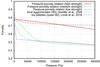 |
Fig. 1 Pressure-porosity relations (crush curve) used in the simulations for the three different sets of parameters (low, medium, high strength) as defined in Table 1. Also shown are the results from laboratory experiments dust agglomerates (Güttler et al. 2009) and ice pebbles (Lorek et al. 2016). |
Material parameters used in the simulations.
2.2. Modeling approach
The modeling approach used here has already been successfully applied in a previous study to the regime of cometesimal collisions (Jutzi & Asphaug 2015). We use a parallel SPH impact code (Benz & Asphaug 1995; Nyffeler 2004; Jutzi et al. 2008; Jutzi 2015) which includes self-gravity as well as material strength models. To avoid numerical rotational instabilities, the scheme suggested by Speith (2006) is used.
In our modeling, we include an initial cohesion Y0> 0 and use a tensile fracture model (Benz & Asphaug 1995), using a range of parameters that lead to an average tensile strength YT varying from ~10 to ~1000 Pa. We consider YT = 100 Pa as the nominal case. To model fractured, granular material, a pressure dependent shear strength (friction) is included by using a standard Drucker-Prager yield criterion (Jutzi 2015). As shown in Jutzi (2015) and Jutzi et al. (2015), granular flow problems are well reproduced using this method.
Porosity is modeled using a P-alpha model (Jutzi et al. 2008) with a simple quadratic crush curve defined by the parameters Pe, Ps, ρ0, ρs0 and α0. We further introduce the density of the compacted material ρcompact = 1980 kg/m3, which is used define the initial distention α0 = ρcompact/ρ0 = 4.5 corresponding to an initial porosity of 1−1 /α0 ~ 78%, consistent with observations (Sierks et al. 2015; Kofman et al. 2015; Pätzold et al. 2016). (We note that ρs0 in this model is a parameter determining the form of the crush curve and does not correspond to the density of the fully compacted material). As an estimate of the compressive strength σc = Ps/2 is used. As shown in Fig. 1, the pressure-porosity relations resulting from these parameters (for low, medium and high strength; Table 1) covers very well the range of experimental curves for dust agglomerates (Güttler et al. 2009) and ice pebbles (Lorek et al. 2016).
We apply a modified Tillotson equation of state (EOS; e.g. Melosh 1989) with parameters for water ice. It is adequate for modeling the collisions considered here, where the most important response is the solid compressibility. As long as there is porosity, the compressibility is limited not by the EOS but by the crush curve of the P-alpha model. The elastic wave speed ce for a porous aggregate body can be very low, of the order of ce ~ 0.1 km s-1. To take this into account, we apply a reduced bulk modulus (leading term in the Tillotson EOS; see Table 1). The approach has the additional major advantage that the time-steps become large enough to carry out the simulations over many dynamical timescales. Different values of ce = 10–100 m/s are investigated.
The relevant material parameters used in the simulations are indicated in Table 1.
2.3. Setup and initial conditions
2.3.1. Impacts on comet 67P and generic bi-lobe shapes
To setup the target, we apply a publicly available shape model of comet 67P1, which defines the surface of the body. Three different sets of material parameters as indicated in Table 1 are used, corresponding to different target strength.
To determine Qreshape for 67P-like shapes, we investigate a range of impact energies using a range of impactor sizes of Rp = 100–300 m and varying the impact velocities. Target and impactor both have the same initial material properties; their initial bulk density is ρ0 ~ 440 kg/m3. We only consider impacts into the smaller of the lobes of comet 67P. Two different impact geometries are investigated (Fig. 2).
To determine the critical shape-changing impact energy Qbil in the case of more general bi-lobe structures, we set up a target consisting of two overlapping ellipsoids (Fig. 6). Each ellipsoid has an axis ratio of 0.6. The volume ratio between the two components is ~0.5 and the total mass of the body is Mt = 1 × 10¹³ kg. For these targets, we only use the nominal set of strength parameters (Table 1) and an impactor size of Rp = 100 m.
The simulations are carried out using a moderately high resolution of ~3 × 10⁵ SPH particles.
2.3.2. Collisions among spherical bodies
In addition to Qreshape and Qbil, we also investigate the critical specific energy for catastrophic disruption of spherical bodies of the same mass and material properties as in the model of comet 67P. To do this we consider 3 different size ratios of projectile and target (1:2; 1:4; 1:8) and varying impact velocities. The impact angle is fixed to 45°.
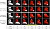 |
Fig. 2 Shape-changing collisions on comet 67P. We use SPH to simulate impacts of a Rp = 100 m projectile on the smaller of the two lobes of comet 67P. The minimal specific energy required to cause a significant change of the comet’s shape by such impacts, Qreshape, is estimated for different impact geometries and rotation axis. The material strength is the same in all cases shown here (YT = 10 Pa). The effect of the material’s sound speed is investigated as well (top row; in this case, a bulk modulus of A = 2.67 × 10⁴ Pa instead of the nominal A = 2.67 × 10⁶ Pa is used). Plotted is a surface of constant density which represents the surface of the comet; shown in red are regions on the surface with materials whose prescribed tensile strength was exceeded. As a rough average, the minimal specific energy required to cause a significant shape change is estimated as Qreshape ~ 0.2 ± 0.1 J/kg, as indicated by the horizontal yellow line. |
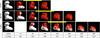 |
Fig. 3 Same as Fig. 2 but for different material strength YT of the target. ce = 100 m/s in all cases. The critical specific energies are: Qreshape ~ 0.2 ± 0.1 J/kg for YT = 10 Pa (corresponds to average in Fig. 2); Qreshape ~ 1.0 ± 0.5 J/kg for YT = 100 Pa; Qreshape ~ 2.0 ± 1.0 J/kg for YT = 1000 Pa. |
2.4. Results
2.4.1. Critical specific energy for shape change
The results of our modeling of impacts on 67P are displayed in Figs. 2–5. We find that this particular structure, with two lobes connected by a neck, is significantly altered even by relatively low energy impacts. For a fixed set of material parameters (i.e. constant strength), the different impact geometries and rotation states considered here lead to slightly different outcomes (Fig. 2), but there are no major, order of magnitude, differences between the various runs.
As it can be observed in Fig. 3, higher material strength lead to higher specific impact energy required to reach a certain degree of change in the overall shape.
There is no unique way to define the critical shape-changing specific impact energy from these results, but rough estimates are possible. Based on visual inspection, we define Qreshape for the different strength as: Qreshape ~ 0.2 ± 0.1 J/kg for YT = 10 Pa; Qreshape ~ 1.0 ± 0.5 J/kg for YT = 100 Pa; Qreshape ~ 2.0 ± 1.0 J/kg for YT = 1000 Pa (Fig. 3) for the impacts with the Rp = 100 m projectile. For the simulations with the larger projectiles we obtain Qreshape ~ 0.3 ± 0.15 J/kg (Rp = 200 m; Fig. 4) and Qreshape ~ 0.15 ± 0.075 J/kg (Rp = 300 m; Fig. 5), using the nominal strength of YT = 100 Pa. These values are plotted in Fig. 7 and compared to the catastrophic disruption threshold, as discussed below. We note that impacts into the larger lobe may lead to slightly different values for Qreshape, but we do not expect order of magnitude differences.
The results of our modeling of impacts on generic bi-lobe shapes (using nominal strength properties) are displayed in Fig. 6. The estimated minimal specific impact energies for reshaping are Qbil ~ 2.0 ± 1.0 J/kg, which is slightly higher than in the case of the 67P-like shape with the same strength (Qbil [YT = 100 Pa] ~ corresponds to Qreshape for the YT = 1000 Pa case).
2.4.2. Catastrophic disruption threshold
The results of our modeling of catastrophic disruptions of spherical bodies with the same mass and material properties as in the model of comet 67P are shown in Fig. 7. We define the specific impact energy as 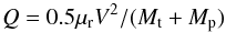 (1)where μr = MpMt/ (Mt + Mp) is the reduced mass, Mp is the mass of the projectile and V the impact velocity. For the oblique (45°) impacts considered here, we also take into account that only a part of the mass of the colliding bodies is interacting (Leinhardt & Stewart 2012), and compute the values of the equivalent head-on collisions.
As expected, the energy threshold for catastrophic disruption  , by ~two orders of magnitude.
As found in previous studies (e.g. Jutzi 2015), in the disruption regime, the results for are almost independent of the material (tensile) strength.
Our values of for different impact velocities (Fig. 7) agree well with scaling law predictions (Housen & Holsapple 1990), adopting a value for the coupling parameter of μ = 0.42, which is typical for porous materials.
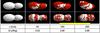 |
Fig. 6 Results of impacts on generic bi-lobe shapes with nominal strength properties (YT = 100 Pa) for two different impact geometries. Rp = 100 m. The minimal specific energy required to cause a significant shape change is estimated as Qbil ~ 2.0 ± 1.0 J/kg. |
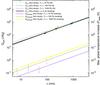 |
Fig. 7 Critical specific impact energies Qcrit. The energy thresholds for shape-changing impacts on a 67P-like shape (Qreshape) for different material strength are shown, as well as the catastrophic disruption energies |
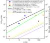 |
Fig. 8 Comparison of critical specific impact energies Qcrit. The scaling laws shown Fig. 7 are compared here with |
The values for the weak, highly porous bodies considered here are slightly higher than the specific energies  found for solid bodies made of strong ice Benz & Asphaug (1999; Fig. 8). This result reflects the dissipative properties of material porosity and is consistent with previous studies (e.g. Jutzi et al. 2010).
Also shown in Fig. 8 is the value of suggested by Leinhardt & Stewart (2009) for weak ice as well as predicted from scaling laws for collisions between gravity-dominated bodies (Leinhardt & Stewart 2012). In these studies, the effects of material porosity were not taken into account.
Finally, we also display in Fig. 8 the specific energies Q involved in collisions of bodies of similar size (mass ratio 1:2) in the bi-lobe forming low-velocity regime investigated by Jutzi & Asphaug (2015). As expected, those low-velocity (V ~ Vesc) accretionary collisions have specific impact energies far below the disruption threshold. For reference, we also show the specific energy for collisions with much higher velocities (v = 40 m/s), which correspond to the average random velocity in the initial primordial disk in the model by Davidsson et al. (2016). For a mass ratio of 1:2, the specific impact energies are even above energy threshold for catastrophic disruptions .
2.5. Scaling laws for critical specific energies
The results obtained in the previous section allow us to derive a scaling law for porous cometary nuclei, which is a function of impact velocity V and target size R (Housen & Holsapple 1990): 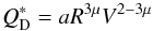 (2)where μ and a are scaling parameters.
For Qreshape and Qbil, we use a fixed target size R = 1800 m. As shown in Fig. 7, μ = 0.42 also reproduces well the velocity dependence of these critical specific energies. The scaling parameters for , Qreshape and Qbil are given in Table 2.
Parameters (SI units) for the scaling law Qcrit = aR3μV2−3μ, where R is the target radius and V the impact velocity.
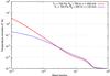 |
Fig. 9 Cumulative post-impact temperature increase dT for two specific cases of shape-changing collisions, as indicated in the plot. |
2.6. Impact heating
The effects of the impacts considered in this study (shape-changing impacts as well as catastrophic disruptions) are analyzed in terms of impact heating and porosity evolution (below). First, in order to get an idea of the maximal global heating, we simply convert the total specific impact energy into a global temperature increase dT = Qcrit/cp where a constant heat capacity cp = 100 J/kg/K is used. The value of cp is a rough mass weighted average of the heat capacity of ice (Klinger 1981) and silicates (Robie & Hemingway 1982) at low temperatures (~30 K), assuming a dust-to-ice mass ratio of 4 (Rotundi et al. 2015). Figures 7 and 8 (scale on the right) shows these dT values corresponding to collisions with a given specific impact energy.
From this simple estimation, it is already obvious that impacts with energies comparable to Qreshape, the maximal global temperature increase must be limited to small values (dT ≪ 1 K). On the other hand, catastrophic impacts at kilometer scales may have the potential to lead to significant large scale heating, depending on how the impact energy is distributed.
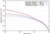 |
Fig. 10 Fraction of material in the final body that experienced a temperature increase larger than a certain value dT in catastrophic disruptions with different velocities V. The mass of the largest remnant Mlr/Mt ~ 50%. Only the material belonging (i.e. which is bound) to the largest remnant is considered in the analysis. |
We compute the actual post-impact dT distribution for a few specific cases of the shape-changing (Sect. 2.4.1) as well as catastrophic collisions (Sect. 2.4.2). In the later, we only consider the material which ends up in the largest remnant (~50% of the initial target mass). The cumulative temperature distribution in the case of the shape-changing impacts (Fig. 9) confirms that only a very small fraction of the material experiences significant heating. For the catastrophic collisions we find that the part of the target which experiences the largest impact effects is ejected. As a result, the material which is bound to the largest remnant (consisting ~50% of the original target mass) is not affected much be the collision (Fig. 10) and the heating is limited (<1% of the mass is heated by dT> 1 K), even at relatively high collision velocities (600 m/s).
2.7. Porosity evolution
Porosity is changed by impacts in multiple ways. First, material is compacted due to the pressure wave generated by the impact. On the other hand, material is ejected and the process of reaccumulation of the gravitationally bound material can give rise to additional macroporosity. Our porosity model computes the degree of compaction (change of the distention variable). In order to specify the increase of the macroporosity, we treat each SPH particle individually according to its ejection/reaccumulation history. Particles which are lifted off the surface or are ejected and reaccumulated experience a density decrease, resulting in an increase of porosity. We assume that reaccumulated material can lead to the addition of macroporosity of maximal 40%, a typical porosity of rubble-pile asteroids (Fujiwara et al. 2006). To compute the total final porosity φtotal resulting from compaction and reaccumulation, we use the relation  (3)and define the distention
  (4)where ρmin is the minimal density reached by the SPH particle and ρcompact = 1980 kg/m3. For this calculation we consider all particles which are gravitationally bound to the main body (largest remnant). The upper limit of the distention is given by
  (5)where αv is the distention value corresponding to 40% macroporosity, αv = (1−φv)-1 with φv = 0.4, and α0 = 4.5 is the initial distention.
The resulting cumulative porosity distributions are calculated for the same cases of shape-changing and catastrophic collisions as discussed in the previous section (Figs. 11 and 12). In the case of the shape-changing collisions, compaction is quite limited, even though the impacted lobe is severely disrupted. Because of the very low gravity, material is lifted off the surface/ejected by the impact. Due to the addition of macroporosity resulting from reaccumulation, the final average porosity is about the same as the initial porosity (Fig. 11).
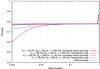 |
Fig. 11 Post-impact porosity distribution for two specific cases of shape-changing collisions, as indicated in the plot. The porosity calculation takes into account compaction as well as the increase of macroporosity. For comparison, the porosity distributions resulting from compaction only are shown as well. The final average porosity (compaction plus addition of macroporosity by reaccumulation) is 78.8% (Rp = 100 m) and 79.2% (Rp = 300 m), respectively, while the initial porosity was 77.8%. |
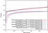 |
Fig. 12 Same as Fig. 11 but for catastrophic collisions. Mlr/Mtot ~ 50%; only the material bound to the largest fragment Mlr is considered. The final average porosity (compaction plus addition of macroporosity by reaccumulation) is 83.3% (V = 10 m/s), 83.3% (V = 100 m/s), 83.3% (V = 200 m/s), 82.4% (V = 800 m/s), respectively, while the initial porosity was 77.8%. |
In the catastrophic disruptions, most of the material which undergoes collisional induced compaction does not remain on the main body (largest remnant). As a result, only ~10% of the material in the final main body has experienced significant compaction. On the other hand reaccumulation plays a major role in this collision regime, resulting in a significant increase of macroporosity. The final porosity is therefore even slightly higher than the initial porosity (Fig. 12).
In Paper II, the interior porosity distribution of bi-lobe structures resulting from sub-catastrophic collisions are compared to observations of comet 67P.
3. The combined dynamical and collisional evolution of comet 67P
3.1. Modeling approach
We follow the approach described in Morbidelli & Rickman (2015) in order to combine the dynamical evolution of the planetesimals precursors of Jupiter family comets with their collisional evolution. We do not repeat here a detailed description of the procedure, but we report on the differences and the improvements in the new implementation.
These are of three kinds. First, we consider here only the dynamical dispersal of the original trans-Neptunian disk of planetesimals, which generates the Scattered Disk (the current source reservoir of JFCs). Thus, we neglect the phase ranging from the time when the gas was removed from the protoplanetary disk to the time when the giant planets developed a dynamical instability that dispersed the planetesimal disk (Tsiganis et al. 2005; Gomes et al. 2005). This choice is made because Morbidelli & Rickman (2015) already showed that in the standard model, a comet the size of 67P has no chance to survive intact during this phase, if protracted for ~400 My. On the other hand the debate on the timing of the giant planet instability is still open (see for instance Kaib & Chambers 2016; Toliou et al. 2016), so it might be possible that the aforementioned phase is short. There is no doubt, however, that the dispersal of the trans-Neptunian disk occurred and that this formed the Scattered Disk. In this case, Morbidelli & Rickman (2015) showed that during this process the number of catastrophic collisions for planetesimals the size of 67P is ~1, so there might be some objects escaping break-up events. Thus, in this work we focus on this case, using improved assessments on the specific energies for catastrophic break-up and for reshaping, described in the previous sections.
The second improvement over Morbidelli & Rickman (2015) concerns the dynamical simulations. Morbidelli & Rickman (2015) used the simulation of Gomes et al. (2005), which covered only the first 350 My after the giant planet instability. This is when most of the action happens, but the subsequent 3.5–4.0 Gy cannot be neglected. Morbidelli & Rickman (2015) assumed that over this remaining time the orbital distribution of the Scattered Disk does not evolve any more, but its population decays exponentially down to 1% of the original population after 4 Gy. The 1% fraction comes from previous studies of the long term evolution of the Scattered Disk (Duncan & Levison 1997). Here we use the simulations presented in Brasser & Morbidelli (2013), which constitute a much more coherent set. Brasser & Morbidelli (2013) studied the dispersal of the trans-Neptunian planetesimal disk during the giant planet instability using a large number of particles (1 080 000; including clones). At the end of the instability, they drove the giant planets towards their exact current orbits, so to avoid artefacts in the subsequent long-term evolution of the Scattered Disk. The evolution of the Scattered Disk was followed for 4 Gy. Because the number of active particles decays over time, the test particles have been cloned 3 times, at 0.2, 1.0 and 3.5 Gy. In the final 0.5 Gy simulation, the particles leaving the Scattered Disk to penetrate into the inner solar system as JFCs have been followed, in order to compare their orbital distribution with that of the observed comets. This final step is crucial to demonstrate that the Scattered Disk generated from the dispersal of the trans-Neptunian disk by the giant planet instability is a valid source of JFCs.
The third improvement over Morbidelli & Rickman (2015) is that the collisional evolution is followed only for the particles that eventually become JFCs in the final 0.5 Gy simulation. These are 87 particles. We think that, potentially, this is an important improvement. The particles that penetrate the inner solar system at the present time might have had specific orbital histories relative to the other particles that either became JFCs much earlier or are still in the Scattered Disk today. Averaging the collisional histories of these three categories of particles may not be significant to address the specific case of 67P, which clearly became JFC only in recent time.
Like in Morbidelli & Rickman (2015) the number of collisions suffered by each considered body is computed assuming that the initial disk particles represent a population of 2 × 10¹¹ planetesimals with diameter D> 2.3 km, with a differential size distribution characterized by an exponent q. The minimum projectile size is determined by the scaling law (Eq. (2)) for the critical specific energy, with parameters given in Table 2. As for the exponent q, in agreement with Morbidelli & Rickman (2015) and previous studies of the comet size distribution, we consider here the cases with q = −2.5,−3.0 and −3.5. However, in the meantime the New Horizons mission to Pluto and Charon has measured the crater size frequency distribution, allowing the assessment of the size distribution of the trans-Neptunian objects larger than a few km in diameter (Singer et al. 2015). The preliminary results2 suggest q = −3.3. Thus, we consider the results for q = −3.0 and −3.5 as the most significant. However, we note that in alternative models (Davidsson et al. 2016) shallower slopes are preferred.
We stress that the approach followed in Morbidelli & Rickman (2015) and in this work is conservative. This means that the number of collisions that are estimated is a lower bound of the real number of collisions. This is because the number of bodies assumed in the initial trans-Neptunian disk (2 × 10¹¹ with D> 2.3 km) is the minimum required, in absence of collisional comminution, to form an Oort cloud and a Scattered disk that contain enough objects to be sufficient sources of the LPC and JFC fluxes that we observe today.
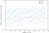 |
Fig. 13 Number of expected catastrophic collisions Ndisrupt during the formation and evolution of the Scattered Disk for the particles that eventually become JFCs in the final 0.5 Gy simulation. Ndisrupt is computed using the scaling parameters for our new |
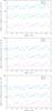 |
Fig. 14 Same as Fig. 13, but shown is the number of shape-changing collisions on a 67P-like body Nreshape, computed using scaling the parameters for Qreshape for different strengths. We note that the number of shape-changing collisions Nbil in the case of a generic bi-lobe shape with nominal strength properties is the same as Nreshape for YT = 1000 Pa (shown in the plot at the bottom). |
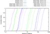 |
Fig. 15 Cumulative fraction of particles (that eventually become JFCs) as a function of the number of collisions. This is an alternative representation of the results already shown in Figs. 13 and 14. The solid lines correspond to the |
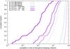 |
Fig. 16 Cumulative fraction of particles (that eventually become JFCs) as a function of the probability P(0) to escape all collisions. The different line styles refer to different exponents for the differential size distribution q, as labeled on the plot. The three curves on the right correspond to the |
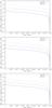 |
Fig. 17 Mean number of reshaping collisions Nreshape expected for 67P-like objects as a function of time for different strengths, as indicated on the y axis. We note that the number of shape-changing collisions Nbil in the case of a generic bi-lobe shape with nominal strength properties is the same as Nreshape for YT = 1000 Pa (bottom). Time t = 0 corresponds to the beginning of the dynamical dispersal of the original trans-Neptunian disk of planetesimals, which generates the Scattered Disk; t = 4 × 10⁹ yr is now. |
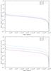 |
Fig. 18 Top: mean number of potential 67P-forming catastrophic collisions of a parent body of R = 3 km (computed using |
3.2. Results: number of disruptive and shape-changing collisions
The number of events for each particle surviving in the Scattered Disk at the end of the disk dispersal simulation is shown in Figs. 13, 14. The results for the various types of collisions, using the corresponding scaling laws ( and Qreshape), are plotted. We note that the results for Qbil (impacts on generic bi-lobe shape using nominal material properties) are the same as in the case of Qreshape with YT = 1000 Pa (Table 2); they are therefore not displayed separately.
Compared to the results by Morbidelli & Rickman (2015), the number of disruptive collisions is smaller (Fig. 13). This is mainly due to the fact the new scaling law used here leads to disruption energies which are higher than the ones by Benz & Asphaug (1999) (which were used in the previous study). As discussed in Sect. 2.4.2, this can be explained by the highly dissipative properties of porous materials, which are taken into account in the new . As Fig. 13 shows, for shallow size distributions, it is possible in principle that a significant fraction of the 67P sized objects escaped all catastrophic collisions.
On the other hand, the number of shape-changing collisions (Fig. 14), requiring a much smaller impact energy (Qreshape), is substantially larger than the number of catastrophic events. As expected, the weaker the strength the larger the number of reshaping collisions taking place. Also, the steeper the size distribution (larger q), the larger the number of collisions happening. However, in any case, even for the largest strength (1000 Pa) and the shallowest slope (q = −2.5), the number of reshaping collisions largely exceeds 1 for all comets.
The results are summarized in Fig. 15 which shows the cumulative fraction of particles as a function of the number of collisions. In Fig. 16, the number of collisions Ncoll is converted into a probability to avoid all collisions P(0) = exp(−Ncoll) and the normalized cumulative distribution of the P(0) values is plotted. The average number of collisions and the related probabilities are given in Table 3.
Average number of shape-changing collision on a 67P-like object (Nreshape), shape-changing collisions on a generic bi-lobe body (Nbil) and catastrophic collisions (Ndisrupt).
It is also interesting to look at the number of collisions as a function of time (Figs. 17 and 18) as this in principle allows us to determine the time at which on average the last event of a certain type took place.
For size distributions with q ≤ −3.0, the last shape-changing event (on average) would have taken place in the last 1 Gy (Fig. 17), suggesting that the structure of comet 67P must have formed in a recent period.
In Fig. 18, we plot the average number of events as a function of time for two potential formation scenarios. In the first scenario, it is assumed that the structure of 67P formed as a result of a catastrophic break-up of a parent body of R = 3 km. The corresponding number of collisions is then computed from our new scaling. In the second case, we consider impact energies corresponding to a scenario of 67P formation by low energy sub-catastrophic collisions, as proposed in Paper II. Clearly, the number of events in the later case are substantially larger. This suggests that it may be a more probable formation mechanism than the catastrophic break-up scenario (see a more detailed discussion on this topic in Paper II).
4. Uncertainties and alternative models
In this section we discuss some aspects of the robustness and uncertainties of our modeling approach and alternative models.
4.1. Critical specific energies
The values for the specific catastrophic disruption energies are well defined and follow the expected scaling (Fig. 7). The critical specific impact energies for reshaping are not as well defined and do depend on the material properties. However, we explore a reasonably large range of material properties and also apply large error bars to the results in this case. In any case, there is no doubt that  and consequently, there must be many more shape-changing events than catastrophic disruptions.
4.2. Dynamical model
A crucial quantity in the dynamical model is the initial number of comets. The assumption of the existence of 2 × 10¹¹ comets is in line with estimates of the current Scattered Disk and Oort cloud populations and numerical estimates of the fractions of the primoridal disk that end up in these populations. Both could be wrong, in principle. However the fractions of the primordial disk population implanted in the Scattered Disk and Oort cloud that we use (from Brasser & Morbidelli 2013) are not very different from those found in quite different dynamical models (Dones et al. 2004 for the Oort cloud to Duncan; and Levison et al. 2008, for the Scattered Disk). Therefore, they seem to be robust.
The number of comets used in our model are based also on a flux of Jupiter family comets which is assumed to be currently in a steady state. If this is not the case, the Scattered Disk could be less (or more) populated than predicted by the model. However, we find this unprobable for the following reason. The current estimates for the populations in the Scattered Disk and the Oort cloud are consistent with these two reservoirs being generated from the same parent disk (Brasser & Morbidelli 2013). Thus, if the Jupiter family comet flux is now – say 10× – the mean flux (so to argue for a Scattered Disk 10× less populated), the same should apply for the flux of long period comets. But the fluxes out of Scattered Disk and Oort cloud follow different processes: for the Scattered Disk, this is resonant diffusion and scattering from Neptune; for the Oort cloud it is stellar perturbations. Therefore, it seems unlikely that both fluxes increased by the same amount relative to the mean values.
Another crucial quantity in our modeling is the slope of the size distribution q, which determines the number of projectiles of a given size and thus the number of impacts with energies above the critical value. There is an ongoing debate about the form of the size distribution in the Scattered Disk population. We argue that the observations of the crater size distributions in the Pluto system by the New Horizons mission provides one of the best available constraints. The cratering of Pluto and Charon is dominated by the hot population (Greenstreet et al. 2015). All models agree that the hot population and the Scattered Disk population are the same population in terms of physical properties and origin. In fact, the collisional evolution of the hot population is not more severe than that of the Scattered Disk. Both suffered most collisions during the dispersal of the primitive disk (or before, if the dispersal was late). It is true that comets have a shallower distribution (Snodgrass et al. 2011) as well as have the craters on the Jovian satellites (Bierhaus 2006; Bierhaus et al. 2009). But this is probably because small comets disintegrate very quickly. On the satellites of Saturn, the crater size distribution is similar to the one expected from a projectile population with a size distribution like that of the main asteroid belt (e.g. Plescia & Boyce 1982; Neukum et al. 2005, 2006), i.e. it is the same as measured by New Horizons on Pluto and Charon.
We note that based on the most recent analysis of the New Horizons data, it has been suggested (Singer et al. 2016) that the size distribution for small (<2 km) objects is shallower (q ≃ −1.5) than at large scales. However, this result is still preliminary with uncertainties to be clarified. As discussed above, the TNO size distribution looks very similar to the size distribution of the asteroid belt, which is a result of a collisional equilibrium (below ~100 km). This suggests that the size distribution of TNOs is in a collisional equilibrium as well. A change of slope below 2 km would produce waves in the TNO size distribution above 2 km. This is not observed, which may indicate that the change of slope is not as pronounced.
To check the effects of a varying slope on our results, we performed additional calculations using q = −3.3 for large (>2 km) and a shallower slope qs for small (<2 km) objects. We find that re-shaping collisions could be avoided for qs ≳ −2, which means that if indeed qs = −1.5, a 67P-like shape would survive. However, we reiterate that this calculation considers a conservative scenario without any collisional evolution in the primordial disk.
4.3. Alternative models
Alternative models to the standard model such as suggested by Davidsson et al. (2016) predict a much smaller collisional evolution and are consistent with the idea of comets being primitive unprocessed objects, formed primordially. However, these models require the number of objects in the Scattered Disk to be orders of magnitude smaller. We note that there is no direct observational measure of the Scattered Disk population and all estimates are indirect and pass through models, so such a small number can in principal not be excluded.
In is not clear, however, how bi-lobe structures would form/survive in these models. Previous studies indicate that the primordial formation of bi-lobed shapes, such as the one of comet 67P, by direct merging requires extremely low collision velocities of V/Vesc ~ 1 (Jutzi & Asphaug 2015). This would have to take place at the very early stages of solar system formation, probably while the gas was still present. In the later phases, relative velocities are much higher. In the model of Davidsson et al. (2016), average relative velocities are V = 40 m/s during the first 25 Myr. For kilometer-sized bodies this implies a ratio V/Vesc ~ 40! In fact, the corresponding specific impact energies are larger than the catastrophic disruption threshold (Fig. 8). Our results show that even relative velocities of a few m/s are destructive and lead to reshaping (Figs. 3–5). Therefore, it is unlikely that primordial bi-lobe structures would survive this phase, and at the same time their formation by collisional merging is implausible due to the high relative velocities.
5. Summary and conclusions
We have estimated the number of shape-changing collisions for an object with a shape like comet 67P, considering a dynamical evolution path typical for a Jupiter family comet, using a “standard model” of the early solar system dynamics.
First, we computed the effects of impacts on comet 67P using a state-of-the-art shock physics code, investigating range of impact conditions and material properties. We found that the shape of comet 67P, with two lobes connected by a neck, can be destroyed easily, even by impacts with a low specific impact energy. From these results, scaling laws for the specific energy required for a significant shape alteration (Qreshape) were developed. For more general applications, the critical specific energies to alter the shape of generic bi-lobe objects (Qbil) was investigated as well.
These scaling laws for Qreshape and Qbil were then used to analyze the dynamical evolution of a 67P-like object and generic bi-lobe shapes in terms of shape-changing collisions. We considered a conservative scenario without any collisional evolution before the dynamical instability of the giant planets. Rather, we tracked the collisions during the dispersion of the trans-Neptunian disk caused by the giant planet instability, the formation of a scattered disk of objects and the penetration of tens of objects into the inner solar system. To do this we used a set of simulations (Brasser & Morbidelli 2013) that produces orbits consistent with the observed JFC population.
We find that even in this conservative scenario, comet 67P would have experienced a significant number of shape-changing collisions, assuming that its structure formed primordially. For size distributions with q ≤ −3.0, the last reshaping event (on average) would have taken place in the last 1 Gy. The preliminary results of the New Horizons missions concerning the crater size-frequency distribution on Pluto and Charon suggest that the current trans-Neptunian population (i.e. including the Scattered Disk) has a differential power-law size distribution with an exponent q ≃ −3.3 (Singer et al. 2015). The possible consequences of a shallower slope for small (<2 km) objects, as suggested recently by Singer et al. (2016), are discussed in Sect. 4.
It has recently been suggested that rotational fission and reconfiguration may be a dominant structural evolution process for short-period comet nuclei with a two-component structure, provided the volume ratio is larger than ~0.2 (Hirabayashi et al. 2016). Our analysis of impacts on generic bi-lobe shapes shows that they would have experienced a substantial number of collisions with energies sufficient to destroy their two-component structure. This strongly suggests that the two-component body which is required to exist at the beginning of the fission-merging cycle cannot be primordial.
Thus, according to our model, comets are not primordial in the sense that their current shape and structure did not form in the initial stages of the formation of the solar system. Rather, they evolve through the effect of collisions and the final shape is a result of the last major reshaping impact, possibly within the last 1 Gy. A scenario of a late formation of 67P-like two-component structures is presented in Paper II.
It is clear that the results presented here are based on the assumption that the standard model of dynamical evolution is correct. Although some of its parameters are debated, as discussed in Sect. 4, we believe that the model is robust. We note that it is so far the only model which produces the correct number of objects in the inner solar system with orbits consistent with the observed JFC population.
Our results clearly show that if this standard model of solar system dynamics is correct, it means that the cometary nuclei as they are observed today must be collisionally processed objects. Therefore, the remaining important question is whether or not such collisionally processed bodies can still have primitive properties (i.e. high porosity, presence of supervolatiles). If this is not the case, then the standard model must be wrong. This would mean for instance that either the primordial disk was dynamically cold and contained a much lower number of objects, as proposed by Davidsson et al. (2016) or that there is a lack of small comets, implying an abrupt change in the slope of the size distribution.
However, the analysis of the outcomes of the detailed impact modeling carried out here (for shape-changing impacts and catastrophic disruptions) suggest that collisionally processed cometary nuclei can still have a high porosity, and could have retained their volatiles, since there is no significant large-scale heating. Therefore, they may still look primitive, meaning that the standard model is consistent with the observations of comet 67P. This question is investigated further in Paper II and also in an ongoing study of bi-lobe formation in large-scale catastrophic disruptions (Schwartz et al., in prep.).
Primordial or not, the structure of comet 67P is an important probe of the dynamical history of small bodies.
We note that based on the most recent results it has been suggested that there may be a deficit of small objects (Singer et al. 2016); see discussion in Sect. 4.
Acknowledgments
M.J. and W.B. acknowledge support from the Swiss NCCR PlanetS. A.T. wishes to thank OCA for their kind hospitality during her stay there. We thank the referees B. Davidsson and J. A. Fernandez for their thorough review which helped improve the paper substantially.
References
- Asphaug, E., & Benz, W. 1994, Nature, 370, 120 [Google Scholar]
- Benz, W., & Asphaug, E. 1995, Comput. Phys. Comm., 87, 253 [Google Scholar]
- Benz, W., & Asphaug, E. 1999, Icarus, 142, 5 [NASA ADS] [CrossRef] [Google Scholar]
- Biele, J., Ulamec, S., Maibaum, M., et al. 2015, Science, 349, aaa9816 [Google Scholar]
- Bierhaus, E. B. 2006, in Workshop on Surface Ages and Histories: Issues in Planetary Chronology, LPI Contributions, 1320, 14 [NASA ADS] [Google Scholar]
- Bierhaus, E. B., Zahnle, K., & Chapman, C. R. 2009, in Europa’s Crater Distributions and Surface Ages, eds. R. T. Pappalardo, W. B. McKinnon, & K. K. Khurana (Tucson: University of Arizona Press), 161 [Google Scholar]
- Boehnhardt, H. 2004, in Comets II (University of Arizona Press), 301 [Google Scholar]
- Brasser, R., & Morbidelli, A. 2013, Icarus, 225, 40 [NASA ADS] [CrossRef] [Google Scholar]
- Capaccioni, F., Coradini, A., Filacchione, G., et al. 2015, Science, 347, aaa0628 [Google Scholar]
- Cuzzi, J. N., Hogan, R. C., & Bottke, W. F. 2010, Icarus, 208, 518 [NASA ADS] [CrossRef] [Google Scholar]
- Davidsson, B. J. R., Sierks, H., Güttler, C., et al. 2016, A&A, 592, A63 [NASA ADS] [CrossRef] [EDP Sciences] [Google Scholar]
- Dones, L., Weissman, P. R., Levison, H. F., & Duncan, M. J. 2004, in Oort cloud formation and dynamics, eds. M. C. Festou, H. U. Keller, & H. A. Weaver (Tucson: University of Arizona Press), 153 [Google Scholar]
- Duncan, M. J., & Levison, H. F. 1997, Science, 276, 1670 [NASA ADS] [CrossRef] [PubMed] [Google Scholar]
- Fujiwara, A., Kawaguchi, J., Yeomans, D. K., et al. 2006, Science, 312, 1330 [NASA ADS] [CrossRef] [PubMed] [Google Scholar]
- Gomes, R., Levison, H. F., Tsiganis, K., & Morbidelli, A. 2005, Nature, 435, 466 [NASA ADS] [CrossRef] [PubMed] [Google Scholar]
- Greenstreet, S., Gladman, B., & McKinnon, W. B. 2015, Icarus, 258, 267 [NASA ADS] [CrossRef] [Google Scholar]
- Güttler, C., Krause, M., Geretshauser, R. J., Speith, R., & Blum, J. 2009, ApJ, 701, 130 [NASA ADS] [CrossRef] [Google Scholar]
- Hässig, M., Altwegg, K., Balsiger, H., et al. 2015, Science, 347, aaa0276 [Google Scholar]
- Hirabayashi, M., Scheeres, D. J., Chesley, S. R., et al. 2016, Nature, 534, 352 [NASA ADS] [CrossRef] [Google Scholar]
- Housen, K. R., & Holsapple, K. A. 1990, Icarus, 84, 226 [NASA ADS] [CrossRef] [Google Scholar]
- Housen, K. R., & Holsapple, K. A. 2003, Icarus, 163, 102 [NASA ADS] [CrossRef] [Google Scholar]
- Johansen, A., Oishi, J. S., Mac Low, M.-M., et al. 2007, Nature, 448, 1022 [Google Scholar]
- Jutzi, M. 2015, Planet. Space Sci., 107, 3 [NASA ADS] [CrossRef] [Google Scholar]
- Jutzi, M., & Asphaug, E. 2015, Science, 348, 1355 [NASA ADS] [CrossRef] [Google Scholar]
- Jutzi, M., & Benz, W. 2017, A&A, 597, A62 (Paper II) [NASA ADS] [CrossRef] [EDP Sciences] [Google Scholar]
- Jutzi, M., Benz, W., & Michel, P. 2008, Icarus, 198, 242 [NASA ADS] [CrossRef] [Google Scholar]
- Jutzi, M., Michel, P., Benz, W., & Richardson, D. C. 2010, Icarus, 207, 54 [NASA ADS] [CrossRef] [Google Scholar]
- Jutzi, M., Holsapple, K. A., Wünnemann, K., & Michel, P. 2015, in Asteroids IV (University of Arizona Press), 679 [Google Scholar]
- Kaib, N. A., & Chambers, J. E. 2016, MNRAS, 455, 3561 [NASA ADS] [CrossRef] [Google Scholar]
- Kataoka, A., Tanaka, H., Okuzumi, S., & Wada, K. 2013, A&A, 557, L4 [NASA ADS] [CrossRef] [EDP Sciences] [Google Scholar]
- Klinger, J. 1981, Icarus, 47, 320 [NASA ADS] [CrossRef] [Google Scholar]
- Kofman, W., Herique, A., Barbin, Y., et al. 2015, Science, 349, aab0639 [Google Scholar]
- Leinhardt, Z. M., & Stewart, S. T. 2009, Icarus, 199, 542 [NASA ADS] [CrossRef] [Google Scholar]
- Leinhardt, Z. M., & Stewart, S. T. 2012, ApJ, 745, 79 [NASA ADS] [CrossRef] [Google Scholar]
- Levison, H. F., Morbidelli, A., Van Laerhoven, C., Gomes, R., & Tsiganis, K. 2008, Icarus, 196, 258 [NASA ADS] [CrossRef] [Google Scholar]
- Lorek, S., Gundlach, B., Lacerda, P., & Blum, J. 2016, A&A, 587, A128 [NASA ADS] [CrossRef] [EDP Sciences] [Google Scholar]
- Massironi, M., Simioni, E., Marzari, F., et al. 2015, Nature, 526, 402 [NASA ADS] [CrossRef] [Google Scholar]
- Melosh, H. J. 1989, Impact cratering: A geologic process (Oxford University Press) [Google Scholar]
- Morbidelli, A., & Rickman, H. 2015, A&A, 583, A43 [NASA ADS] [CrossRef] [EDP Sciences] [Google Scholar]
- Morbidelli, A., Bottke, W. F., Nesvorný, D., & Levison, H. F. 2009, Icarus, 204, 558 [NASA ADS] [CrossRef] [Google Scholar]
- Morbidelli, A., Marchi, S., Bottke, W. F., & Kring, D. A. 2012, Earth Planet. Sci. Lett., 355, 144 [NASA ADS] [CrossRef] [Google Scholar]
- Mumma, M. J., Weissman, P. R., & Stern, S. A. 1993, in Protostars and Planets III, 1177 [Google Scholar]
- Neukum, G., Wagner, R. J., Denk, T., Porco, C. C., & Cassini Iss Team 2005, in 36th Annual Lunar and Planetary Science Conf., eds. S. Mackwell, & E. Stansbery, Lunar and Planetary Inst. Tech. Rep., 36 [Google Scholar]
- Neukum, G., Wagner, R., Wolf, U., & Denk, T. 2006, in Eur. Planet. Sci. Cong., 610 [Google Scholar]
- Nyffeler, B. 2004, Ph.D. Thesis, University of Bern, Switzerland [Google Scholar]
- Pätzold, M., Andert, T., Hahn, M., et al. 2016, Nature, 530, 63 [NASA ADS] [CrossRef] [Google Scholar]
- Plescia, J. B., & Boyce, J. M. 1982, Nature, 295, 285 [NASA ADS] [CrossRef] [Google Scholar]
- Rickman, H., Marchi, S., A’Hearn, M. F., et al. 2015, A&A, 583, A44 [NASA ADS] [CrossRef] [EDP Sciences] [Google Scholar]
- Robie, A., & Hemingway, B. 1982, American Mineralogist, 67, 470 [Google Scholar]
- Rotundi, A., Sierks, H., Della Corte, V., et al. 2015, Science, 347, aaa3905 [Google Scholar]
- Sierks, H., Barbieri, C., Lamy, P. L., et al. 2015, Science, 347, aaa1044 [Google Scholar]
- Singer, K. N., Schenk, P. M., Robbins, S. J., et al. 2015, in AAS/Division for Planetary Sciences Meeting Abstracts, 47, 102.02 [Google Scholar]
- Singer, K. N., McKinnon, W. B., Greenstreet, S., et al. 2016, in AAS/Division for Planetary Sciences Meeting Abstracts, 48, 213.12 [Google Scholar]
- Skorov, Y., & Blum, J. 2012, Icarus, 221, 1 [NASA ADS] [CrossRef] [Google Scholar]
- Snodgrass, C., Fitzsimmons, A., Lowry, S. C., & Weissman, P. 2011, MNRAS, 414, 458 [NASA ADS] [CrossRef] [Google Scholar]
- Speith, R. 2006, Habilitation, University of Tübingen, Germany [Google Scholar]
- Steckloff, J. K., Johnson, B. C., Bowling, T., et al. 2015, Icarus, 258, 430 [NASA ADS] [CrossRef] [Google Scholar]
- Toliou, A., Morbidelli, A., & Tsiganis, K. 2016, A&A, 592, A72 [NASA ADS] [CrossRef] [EDP Sciences] [Google Scholar]
- Tsiganis, K., Gomes, R., Morbidelli, A., & Levison, H. F. 2005, Nature, 435, 459 [NASA ADS] [CrossRef] [PubMed] [Google Scholar]
- Weidenschilling, S. J. 1997, Icarus, 127, 290 [NASA ADS] [CrossRef] [Google Scholar]
- Weissman, P. R., Asphaug, E., & Lowry, S. C. 2004, in Comets II (Tucson: University of Arizona Press), 337 [Google Scholar]
- Windmark, F., Birnstiel, T., Güttler, C., et al. 2012a, A&A, 540, A73 [NASA ADS] [CrossRef] [EDP Sciences] [Google Scholar]
- Windmark, F., Birnstiel, T., Ormel, C. W., & Dullemond, C. P. 2012b, A&A, 544, L16 [NASA ADS] [CrossRef] [EDP Sciences] [Google Scholar]
- Youdin, A. N., & Goodman, J. 2005, ApJ, 620, 459 [NASA ADS] [CrossRef] [Google Scholar]
All Tables
Parameters (SI units) for the scaling law Qcrit = aR3μV2−3μ, where R is the target radius and V the impact velocity.
Average number of shape-changing collision on a 67P-like object (Nreshape), shape-changing collisions on a generic bi-lobe body (Nbil) and catastrophic collisions (Ndisrupt).
All Figures
|
Fig. 1 Pressure-porosity relations (crush curve) used in the simulations for the three different sets of parameters (low, medium, high strength) as defined in Table 1. Also shown are the results from laboratory experiments dust agglomerates (Güttler et al. 2009) and ice pebbles (Lorek et al. 2016). |
| In the text | |
|
Fig. 2 Shape-changing collisions on comet 67P. We use SPH to simulate impacts of a Rp = 100 m projectile on the smaller of the two lobes of comet 67P. The minimal specific energy required to cause a significant change of the comet’s shape by such impacts, Qreshape, is estimated for different impact geometries and rotation axis. The material strength is the same in all cases shown here (YT = 10 Pa). The effect of the material’s sound speed is investigated as well (top row; in this case, a bulk modulus of A = 2.67 × 10⁴ Pa instead of the nominal A = 2.67 × 10⁶ Pa is used). Plotted is a surface of constant density which represents the surface of the comet; shown in red are regions on the surface with materials whose prescribed tensile strength was exceeded. As a rough average, the minimal specific energy required to cause a significant shape change is estimated as Qreshape ~ 0.2 ± 0.1 J/kg, as indicated by the horizontal yellow line. |
| In the text | |
|
Fig. 3 Same as Fig. 2 but for different material strength YT of the target. ce = 100 m/s in all cases. The critical specific energies are: Qreshape ~ 0.2 ± 0.1 J/kg for YT = 10 Pa (corresponds to average in Fig. 2); Qreshape ~ 1.0 ± 0.5 J/kg for YT = 100 Pa; Qreshape ~ 2.0 ± 1.0 J/kg for YT = 1000 Pa. |
| In the text | |
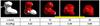 |
Fig. 4 Same as Fig. 3 but for Rp = 200 m (YT = 100 Pa). Qreshape ~ 0.3 ± 0.15 J/kg. |
| In the text | |
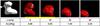 |
Fig. 5 Same as Fig. 3 but for Rp = 300 m (YT = 100 Pa). Qreshape ~ 0.15 ± 0.075 J/kg. |
| In the text | |
|
Fig. 6 Results of impacts on generic bi-lobe shapes with nominal strength properties (YT = 100 Pa) for two different impact geometries. Rp = 100 m. The minimal specific energy required to cause a significant shape change is estimated as Qbil ~ 2.0 ± 1.0 J/kg. |
| In the text | |
|
Fig. 7 Critical specific impact energies Qcrit. The energy thresholds for shape-changing impacts on a 67P-like shape (Qreshape) for different material strength are shown, as well as the catastrophic disruption energies |
| In the text | |
|
Fig. 8 Comparison of critical specific impact energies Qcrit. The scaling laws shown Fig. 7 are compared here with |
| In the text | |
|
Fig. 9 Cumulative post-impact temperature increase dT for two specific cases of shape-changing collisions, as indicated in the plot. |
| In the text | |
|
Fig. 10 Fraction of material in the final body that experienced a temperature increase larger than a certain value dT in catastrophic disruptions with different velocities V. The mass of the largest remnant Mlr/Mt ~ 50%. Only the material belonging (i.e. which is bound) to the largest remnant is considered in the analysis. |
| In the text | |
|
Fig. 11 Post-impact porosity distribution for two specific cases of shape-changing collisions, as indicated in the plot. The porosity calculation takes into account compaction as well as the increase of macroporosity. For comparison, the porosity distributions resulting from compaction only are shown as well. The final average porosity (compaction plus addition of macroporosity by reaccumulation) is 78.8% (Rp = 100 m) and 79.2% (Rp = 300 m), respectively, while the initial porosity was 77.8%. |
| In the text | |
|
Fig. 12 Same as Fig. 11 but for catastrophic collisions. Mlr/Mtot ~ 50%; only the material bound to the largest fragment Mlr is considered. The final average porosity (compaction plus addition of macroporosity by reaccumulation) is 83.3% (V = 10 m/s), 83.3% (V = 100 m/s), 83.3% (V = 200 m/s), 82.4% (V = 800 m/s), respectively, while the initial porosity was 77.8%. |
| In the text | |
|
Fig. 13 Number of expected catastrophic collisions Ndisrupt during the formation and evolution of the Scattered Disk for the particles that eventually become JFCs in the final 0.5 Gy simulation. Ndisrupt is computed using the scaling parameters for our new |
| In the text | |
|
Fig. 14 Same as Fig. 13, but shown is the number of shape-changing collisions on a 67P-like body Nreshape, computed using scaling the parameters for Qreshape for different strengths. We note that the number of shape-changing collisions Nbil in the case of a generic bi-lobe shape with nominal strength properties is the same as Nreshape for YT = 1000 Pa (shown in the plot at the bottom). |
| In the text | |
|
Fig. 15 Cumulative fraction of particles (that eventually become JFCs) as a function of the number of collisions. This is an alternative representation of the results already shown in Figs. 13 and 14. The solid lines correspond to the |
| In the text | |
|
Fig. 16 Cumulative fraction of particles (that eventually become JFCs) as a function of the probability P(0) to escape all collisions. The different line styles refer to different exponents for the differential size distribution q, as labeled on the plot. The three curves on the right correspond to the |
| In the text | |
|
Fig. 17 Mean number of reshaping collisions Nreshape expected for 67P-like objects as a function of time for different strengths, as indicated on the y axis. We note that the number of shape-changing collisions Nbil in the case of a generic bi-lobe shape with nominal strength properties is the same as Nreshape for YT = 1000 Pa (bottom). Time t = 0 corresponds to the beginning of the dynamical dispersal of the original trans-Neptunian disk of planetesimals, which generates the Scattered Disk; t = 4 × 10⁹ yr is now. |
| In the text | |
|
Fig. 18 Top: mean number of potential 67P-forming catastrophic collisions of a parent body of R = 3 km (computed using |
| In the text | |
Current usage metrics show cumulative count of Article Views (full-text article views including HTML views, PDF and ePub downloads, according to the available data) and Abstracts Views on Vision4Press platform.
Data correspond to usage on the plateform after 2015. The current usage metrics is available 48-96 hours after online publication and is updated daily on week days.
Initial download of the metrics may take a while.