| Issue |
A&A
Volume 597, January 2017
|
|
|---|---|---|
| Article Number | A36 | |
| Number of page(s) | 7 | |
| Section | Catalogs and data | |
| DOI | https://doi.org/10.1051/0004-6361/201527753 | |
| Published online | 20 December 2016 | |
K2P2: Reduced data from campaigns 0–4 of the K2 mission
1 Stellar Astrophysics Centre, Department of Physics and AstronomyAarhus University, Ny Munkegade 120, 8000 Aarhus C, Denmark
e-mail: This email address is being protected from spambots. You need JavaScript enabled to view it.
2 School of Physics and Astronomy, University of Birmingham, Edgbaston, Birmingham, B15 2TT, UK
e-mail: This email address is being protected from spambots. You need JavaScript enabled to view it.
Received: 16 November 2015
Accepted: 17 August 2016
Abstract
Context. After the loss of a second reaction wheel the Kepler mission was redesigned as the K2 mission, pointing towards the ecliptic and delivering data for new fields approximately every 80 days. The steady flow of data obtained with a reduced pointing stability calls for dedicated pipelines for extracting light curves and correcting these for use in, e.g., asteroseismic analysis.
Aims. We provide corrected light curves for the K2 fields observed until now (campaigns 0–4), and provide a comparison with other pipelines for K2 data extraction/correction.
Methods. Raw light curves are extracted from K2 pixel data using the “K2-pixel-photometry” (K2P2) pipeline, and corrected using the KASOC filter.
Results. The use of K2P2 allows for the extraction of the order of 90 000 targets in addition to 70 000 targets proposed by the community – for these, other pipelines provide no data. We find that K2P2 in general performs as well as, or better than, other pipelines for the tested metrics of photometric quality. In addition to stars, pixel masks are properly defined using K2P2 for extended objects such as galaxies for which light curves are also extracted.
Key words: methods: data analysis / stars: oscillations
© ESO, 2016
1. Introduction
During May of 2013 a second of four on-board reaction wheels of the Kepler spacecraft was lost and with it the ability to maintain 3-axis pointing stability of the spacecraft. This led to the redesigned mission “K2” where fields towards the ecliptic are observed for a duration of approximately 80 days (Howell et al. 2014). The specific challenges with data quality, combined with the high and steady flow of data from the K2 mission calls for dedicated data analysis pipelines to deliver data to the community.
We here report on the release of light curves extracted from raw pixel data from K2’s Campaigns (C) 0–4 using masks defined by the K2-pixel-photometry (K2P2) pipeline presented in Lund et al. (2015, hereafter L15). Corrections of the resulting raw light curves are made using the KASOC pipeline by Handberg & Lund (2014, hereafter HL14). This paper will serve as a data release note, describing the characteristics of the data and the reduced products that have been made available via the KASOC database1.
Our paper is structured as follows. In Sects. 2 and 3 we briefly describe the concept of the K2P2 pipeline, and the KASOC pipeline which removes systematic artefacts. Here we also report on the properties of the pipeline segment pertaining to defining masks and estimating magnitudes. Section 4 reports on characteristics of the extracted light curves, focusing on noise properties. We detail in Sect. 5 the data products that have been made available on KASOC and summarise in Sect. 7 with an outlook on future potential updates to the pipeline.
2. Light curve extraction (K2P2)
Raw light curves were extracted from K2 pixel data from C0–4 using the K2P2 pipeline L15. Briefly, K2P2 defines pixel masks from a time-summed image of a given EPIC postage stamp where the background has been corrected for. In the summed image, potential pixels to include in defining the pixel masks are then selected based on a flux threshold; clusters in these pixels, each seen as an individual target in the frame, are then located using an unsupervised clustering algorithm; for each pixel-cluster an image-segmentation algorithm is run to segment clusters containing two or more close targets. From the identified targets we extract the flux together with the flux-weighted centroid as a function of time for subsequent correction of the light curves (see Sect. 3 below).
We note the following modifications to K2P2 as compared to L15: (1) from C3 onwards background subtraction has been performed by the K2 Science Team on the raw pixel data, so from C3 this step is omitted in the data extraction; (2) from C3 onwards centroids provided in the pixel data (see Sect. 3) are used instead of flux weighted centroids calculated from individual targets. The centroids provided in the target pixel data are computed from a select number of bright (non-saturated) targets in the field-of-view (FOV) of the given campaign; the centroids for these targets are then interpolated to the positions of other targets. Generally, the centroids calculated in this manner show a lower scatter than the ones calculated from individual targets, particularly for saturated targets.
For recent applications of the K2P2 pipeline we refer to Stello et al. (2015), Chaplin et al. (2015), Kurtz et al. (2016), Lund et al. (2016a,b), and Miglio et al. (2016). For other K2 data extraction and correction pipelines we refer to Vanderburg & Johnson (2014), Vanderburg (2014), Aigrain et al. (2015, 2016), Foreman-Mackey et al. (2015), Huang et al. (2015), Armstrong et al. (2015, 2016), Van Cleve et al. (2016), Buzasi et al. (2015), and Libralato et al. (2016).
2.1. Magnitude estimation
As described in L15 (see also Aigrain et al. 2015) we estimate a proxy for the Kepler magnitude,  , as
, as  (1)where S denotes the median of the flux time series extracted for the target (in units of e−/ s). The relation between these magnitudes and the Kepler magnitude provided in the EPIC, KpEPIC, is shown in Fig. 1 for C0–4 long-cadence (LC; Δt ≈ 29.4 m) targets. The different marker colours correspond to the bandpass magnitude(s) used to estimate KpEPIC following the relations presented in Brown et al. (2011), Howell et al. (2012), and Huber & Bryson (2015). We note that in C0 the KpEPIC was simply given by the input magnitude from the principal investigator proposing a given target, hence these are often simply given by the bandpass magnitude(s) without a proper conversion to the Kepler bandpass. We use the KepFlag entry of the EPIC (not defined in C0) to obtain the source for the computed KpEPIC.
Overall, we see a good agreement between KpEEPIC and especially for KpEPIC ≲ 13. Exceptions to this are seen for smaller groups of targets, typically computed from specific bandpass magnitudes – we refer to the release notes2 for known problems with KpEPIC magnitudes for different campaigns. We note that targets with masks containing stars not in the EPIC will likely have a positive difference in Fig. 1 as the flux from these targets is naturally combined in but unaccounted for in KpEPIC which only combine the magnitudes from targets found in the EPIC.
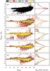 |
Fig. 1 Comparison between Kepler magnitudes from the EPIC (KpEPIC) and the proxy magnitude |
2.2. Target identification and statistics
The K2P2 pipeline allows for the extraction of data for all targets in a given frame, not only the targets associated with the EPIC (Ecliptic Plane Input Catalog; Huber & Bryson 2015) identifier for the frame. If more than one target is found in a given frame the additional targets will also often have an EPIC identifier and may also be found in a separate frame associated with that EPIC; other times the target has an EPIC ID but has not been proposed for observations. Targets in this latter case would normally be ignored, but can be treated with the K2P2 pipeline.
The problem of identifying the extracted targets is handled by matching all the extracted targets against the EPIC catalog, which itself is a compilation of several other catalogs. Corrections to the world coordinate solutions (see also Sect. 2.4) are calculated using the full EPIC catalog as described in L15 and targets with corrected positions falling within each aperture are assigned to that aperture. All EPIC IDs which falls within the aperture are stored and used to calculate diagnostic information like contamination metrics and the expected brightness, but only the EPIC ID with the brightest Kepler magnitude is in the end assigned to the aperture.
For the processing of K2 data reported here, a target must fulfil all of the following requirements in order to be finally validated:
-
1.
A pixel mask must contain a minimum of 8 pixels.
-
2.
An aperture must be assigned to an EPIC ID.
-
3.
In a given frame, one of the apertures must be assigned to the main EPIC ID.
-
4.
If an EPIC ID is associated to more than one extracted pixel mask, only the pixel mask with the largest distance to the edge of the given pixel frame is kept.
-
5.
If the aperture assigned to the main EPIC ID fails any of the above requirements, all extracted apertures from that frame are rejected.
It should be noted that in this release we are depending on the completeness of the EPIC catalogue for the second requirement to be fulfilled. In the future we will be able to provide new targets to the EPIC by matching the measured position and of a given identified target to catalogues not currently included in the EPIC and feed this information back to the K2 science office.
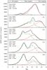 |
Fig. 2 Kernel density estimates (KDE) for the number of targets (with |

Figure 2 gives the kernel density estimates (KDEs) for the number of extracted LC targets against for the different campaigns. With K2P2 a significant distribution of additional targets (peaking around  ) is added to the distribution of proposed targets. In C0 the addition of targets is in excess of 750%, while the average addition for following campaigns is around 56%. This amounts to an additional ~ 90 000 targets (~ 37 000 not counting C0); the number of proposed targets amounts to ~ 70 000 (~ 63 000 not counting C0). A clear decreasing trend is seen in the percentage addition of targets with advancing campaigns, because the number of pixels in the so-called “postage stamps” around targets has been decreased to optimise the overall pixel budget of the mission.
2.3. Properties of pixel masks
The size of the pixel masks defined by K2P2 is determined by how the flux is distributed for individual targets. One would therefore expect a strong correlation and smoothly varying change in mask size with the stellar magnitude. In Fig. 3 we show the mask sizes as a function of obtained for LC targets in C3; as mentioned in Sect. 2.2 a lower limit on the mask size was set to 8 pixels. A correlation is seen as expected, and as noted in L15 a slight gradient is seen in the mask size with the distance to the spacecraft bore sight from the increase in roll angle. A tail of dim targets with high magnitudes and large mask sizes is also apparent (marked with black crosses). All of these targets were proposed in the guest observer (GO) proposal 3048 (“The KEGS Transient Survey”), and are all truly extended objects such as galaxies which cannot be expected to follow the same variation as stellar targets. We note that these targets are in the EPIC entry “Object type” listed as “STAR” (rather than “EXTENDED”), so care should be exerted when analysing large ensembles of targets from K2 if only the EPIC is used to make the target selection. An example of an extended object (here EPIC 206028594 or NGC 7300) is shown in Fig. 4 – as seen, the K2P2 pipeline defines masks for this type of object without any issues or modifications needed. Here we see a disadvantage for this type of target from using the Kepler photometric analysis (PA) module or the Harvard pipeline (Vanderburg & Johnson 2014) to define masks, which depends on the adopted Kepler magnitude assuming a stellar target.
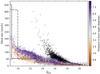 |
Fig. 3 Pixel mask siz es versus the proxy Kepler magnitude |
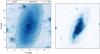 |
Fig. 4 Left: pixel frame for EPIC 206028594, also known as NGC 7300; the colour goes from white (low flux) to blue (high flux). Indicated are the masks defined by K2P2, the Harvard pipeline (Vanderburg & Johnson 2014), and the photometric analysis (PA) component of the Kepler science processing pipeline (Bryson et al. 2010). We also show (with red masks) the two other targets identified by K2P2 under the constraint of a minimum pixel mask of 8 pixels. Right: image of NGC 7300 from the Southern Sky Atlas (SERC), with colours and orientation modified to match in appearance the K2 data. |
The panels of Fig. 5 gives the median binned mask sizes – excluding targets from galaxy/AGN surveys3 – for different campaigns and pipelines, together with the interquartile range (IQR) for the mask sizes. We see for K2P2 a very stable relationship between mask sizes and (left panel). We also show the mask size relation obtained by Aigrain et al. (2015) from engineering data, by Armstrong et al. (2015) from C0 (where we note that the authors used Kp magnitudes without re-calibration), and mask sizes extracted from the reduced light curves by the Harvard pipeline4 (middle panel). From the Harvard pipeline we adopt the mask given as the “Best” in their FITS files, but have only included in Fig. 5 the masks defined from pixel-response-function (PRF) fits; the circular masks from the Harvard pipeline for C0 data often span a large range of mask sizes for a given magnitude, with the distinct risk of having multiple targets in a given mask. In general we find that the Vanderburg & Johnson (2014) masks are smaller than the ones from K2P2. The right panel shows the mask sizes obtained from the PA component of the Kepler science processing pipeline. For these we again see masks smaller than those from K2P2, and notice a change in the definition of mask sizes with magnitude between C2 and C3 where a jump in mask size is seen around Kp ≈ 11 from C3 onwards. For both the Harvard and PA masks no noticeable deviation in sizes is seen for the extended objects mentioned above (black crosses in right panel). We also note the allowance in the PA data for masks down to a single pixel, whilst we in K2P2 set a lower limit of 8 pixels.
 |
Fig. 5 Comparison between the median binned mask sizes for Campaigns 0–4 excluding targets from AGN/galaxy GO proposals3; hatch-shaded regions indicate the IQR for the mask sizes. For a better visualisation we only show the comparison for |

2.4. The world coordinate system
In L15 a correction was introduced to the world-coordinate-system (WCS) provided in the target pixel data. Figure 6 presents the obtained absolute correction in pixels to the expected position of targets from the WCS. We see that the needed correction was the largest in C0, but with later updates to the WCS the correction is seen to drop below 0.4 pixel. Depending on the crowding of the specific campaign this level of off-set should in general be small enough to correctly identify targets in the frames. As a consequence of this we have changed the maximal shift we allow in the positions to one pixel from C3 and onward.
3. Light curve corrections (KASOC Filter)
The raw light curves are corrected using the KASOC filter (L15) incorporating a correction for the systematics from the varying roll angle of the spacecraft in a manner mimicking the self-flat-fielding method by Vanderburg & Johnson (2014). The only differences compared to the description of the 1D-correction provided in L15 are (1) the use of centroids from the target pixel files (from C3 onwards) – these can be found in the POS_CORR columns of the target pixel files; (2) the use of the following new “Quality” bits: 17 (decimal = 65 536; “No data reported”) and 19 5 (decimal = 262 144; “Definite Thruster Firing”) for which we exclude the data points. We refer to HL14 for further details on the KASOC filter.
4. Noise properties
Here we present the results obtained for noise characteristics of the filtered data. We consider five frequently used indicators for photometric variability, namely, (1) the point-to-point median difference variability (MDV), given by the median of the time series of point-to-point differences of the corrected light curve (Basri et al. 2011); (2) the 6.5-h combined differential photometric precision (CDPP6.5h), obtained in a manner similar to Gilliland et al. (2011), i.e., by applying the combined spectral response of a 6.5-h Savitzky-Golay (SG) filter (Savitzky & Golay 1964) and a 2-day boxcar filer to the un-weighted power spectrum of the filtered light curve (see also Christiansen et al. 2012) – following the Parseval-Plancherel theorem (Parseval des Chênes 1806; Plancherel 1910) the CDPP6.5h gives the root-mean-squared scatter of the time series on time scales around 6.5 h; (3) the 24-day “long-CDPP” (CDPP24d), which uses a 24-day SG filter together with a 3.25-day boxcar (Gilliland et al. 2015). This metric is better suited to capture stellar activity variations by giving a measure for the photometric variability on time scales between 8−15 days; (4) the 6.5-h “quasi-CDPP” metric reported in Vanderburg & Johnson (2014) and Aigrain et al. (2015). This metric is calculated from the median of the rolling 6.5-h (13 LC cadences) standard deviation divided by  – this therefore gives the median of the error on the mean in 6.5-h window, which is different from the definition of the CDPP by Gilliland et al. (2011). In many ways this metric is close to the point-to-point MDV metric, and is in using the median largely insensitive to any non-stationary components in the corrected light curve, such as residual trends from the ~ 6-h pointing correction; (5) the median level of the power spectrum from corrected light curves between 260 and 280 μHz.
To allow for a comparison with data from the Harvard pipeline and from the Kepler PA module we have computed the five metrics listed above in a uniform manner for all data sets. From the PA module only C3–4 corrected data have been made available. For the computations of metrics 2, 3, and 5 a un-weighted power spectrum was used. In the data that will be made available we will also include a weighted power spectrum, which likely will have lower values for metric 5 (see Sect. 5).
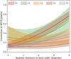 |
Fig. 6 Absolute correction in pixels to the estimated position of targets, based on the WCS provided in target pixel files, as a function of angular distance to the spacecraft bore sight. The hatched-shaded region per campaign indicate the IQR of the pixel correction. |
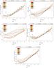 |
Fig. 7 Comparison of photometric variability metrics between the K2P2, Harvard (C0–4), and PA (C3–4) pipelines as a function of Kp ( |
Figure 7 gives the computed metrics as a function of Kp (for Harvard and PA) or (for K2P2); the plotted values give the median binned values of the different metrics. For CDPP6.5h we include a comparison with the lower envelope of this metric from the nominal Kepler mission, obtained as the 1st percentile from 0.3 mag wide bins of the values in Gilliland et al. (2011, their Fig. 4).
We see that in general K2P2 returns lower values for the metrics 2, 3, and 5 across the full magnitude range; for metrics 1 and 4 the results from the different pipelines are overall in agreement with each other. The PA results typically lie in-between the Harvard and K2P2 values. Of particular interest to asteroseismic studies we see that for metric 5, the median value of the power spectrum between 260 and 280 μHz, drops by a factor of ~ 10 between C0 and C3 for  ; this should enable a significant increase in the detectability of oscillations for evolved stars (see Stello et al. (2015) for seismic studies of red giants in C1). We stress that any metric of photometric variability used to assess the “quality” of the light curves should be considered in the context of their intended use. The optimal light curve for asteroseismic studies is different from, for instance, that sought for in planetary studies. Also, the metrics will be influenced by the definition of pixel masks.
5. Data products
We will make corrected light curves available on the KASOC database, together with both weighted and unweighted power spectra as described in HL14. The formatting of the FITS files will generally follow that described in HL14. Besides the extensions mentioned in HL14 the FITS files will have the added extension “APERTURE” which contains an image of the K2P2 pixel mask. We have added the following columns (all in in e−/s) to the binary table belonging to the “LIGHTCURVE” extension in order to expand on the “FILTER” column containing the full KASOC filter: “XLONG”, “XSHORT”, “XPOS”, “XPHASE”, and “FLUX_RAW”. These contain respectively the τlong and τshort filter components, the positional correction to the roll of the spacecraft in K2, the phase-folded component (used if light curve contains transits with known period(s)), and lastly the raw uncorrected light curve. The first four components are constructed such that their sum equals “FILTER”.
We have added the entries listed in Table 1 to the “PRIMARY” extension holding a header containing information on the star, the data used, and the adopted filter parameters for the given star. See HL14 for the reminder of the entries supplied, and L15 for explanations to the K2P2 related entries.
6. Data policies
If you use the data that have been produced during this release in your scientific works, we kindly request
-
To add the following sentence: “The Kepler light curves used inthis work has been extracted using the pixel data following themethods described in Lundet al. (2015) and correctedfollowing Handberg & Lund (2014)”.
-
We request the following sentences be added to the acknowledgements section: “This research has made use of the KASOC database, operated from the Stellar Astrophysics Centre (SAC) at Aarhus University, Denmark. Funding for the Stellar Astrophysics Centre (SAC) is provided by The Danish National Research Foundation. The research is supported by the ASTERoseismic Investigations with SONG and Kepler project (ASTERISK) funded by the European Research Council (Grant agreement No.: 267864)”.
-
If extra work was required to produce the data used, like tweaking of filter parameters or similar, we request to be added to the author list of any publications using such specially prepared data.
Special keywords in the first/primary extension of the FITS files.
7. Summary and outlook
We have presented characteristics of light curves from K2 campaigns 0–4 extracted using the K2P2 pipeline – these light curves, and their power spectra, will be made available on the KASOC database. In terms of the data extraction the K2P2 pipeline performs very well, quantified by an addition of ~ 90 000 extra light curves from untargeted stars for which data would not have been available otherwise. Concerning the definition of pixel masks a correlation as expected is obtained between mask sizes and target brightness, and contrary to other pipelines, masks are properly defined even for extended objects such as galaxies. The use of K2P2 light curves would thus increase the likelihood of detecting signals from supernovas and AGNs in these extragalactic targets. The extracted light curves are corrected using the KASOC Filter pipeline, and we find that these overall have lower photometric variability than those from other pipelines – this could impact the detectability of, for instance, seismic signals. For K2P2 light curves a median drop in our proxy for white noise (see metric 5 in Sect. 4) by a factor of ~ 10 between C0 and C3 for  , which should positively affect the detection of oscillations from red giants.
For future light curve processing we note that the use of house-keeping data from the Kepler spacecraft could improve light curve corrections, because this would allow for a complete mapping between CCD position and apparent movement on the CCD without the need for computing stellar centroids.
We find that the concept of K2P2 holds great potential for use with the upcoming NASA Transiting Exoplanet Survey Satellite
mission (TESS; Ricker et al. 2014). TESS will deliver full frame images of a 24° × 96° FOV with a cadence of ~ 30 min for a duration of 27 days per field – here an automatic and robust definition of pixels masks for targets in the FOV will be needed for the optimal utilisation of TESS data.
We have removed targets from the following GO proposals (see http://keplerscience.arc.nasa.gov/k2-fields.html): 0009, 0061, 0103, 0106, 1025, 1035, 1072, 1074, 2004, 3004, 3033, 3048, 4038, 4096, 4100.
Obtained from The Mikulski Archive for Space Telescopes (MAST).
This bit is listed as “21” in the pipeline release notes (http://keplerscience.arc.nasa.gov/K2/pipelineReleaseNotes.shtml) which we believe to be an error.
Acknowledgments
The authors wish to thank the entire Kepler and K2 teams, without whom these results would not be possible. We are grateful to Ronald L. Gilliland for data provided for the comparison of K2 and nominal Kepler CDPP, and to Thomas Barclay for answering questions on the K2 data products. “Ta” to Bill Chaplin for giving comments to a draft of this paper.
Funding for the Stellar Astrophysics Centre (SAC) is provided by The Danish National Research Foundation. The research is supported by the ASTERISK project (ASTERoseismic Investigations with SONG and Kepler) funded by the European Research Council (Grant agreement No.: 267864).
M.N.L. acknowledges the support of The Danish Council for Independent Research | Natural Science (Grant DFF-4181-00415). M.N.L. was partly funded by the European Community’s Seventh Framework Programme (FP7/2007−2013) under grant agreement No. 312844 (SPACEINN), which is gratefully acknowledged.
This research has made use of the following web resources: the SIMBAD database, operated at CDS, Strasbourg, France; NASAs Astrophysics Data System Bibliographic Services; the Mikulski Archive for Space Telescopes (MAST); ArXiv, maintained and operated by the Cornell University Library.
References
- Aigrain, S., Hodgkin, S. T., Irwin, M. J., Lewis, J. R., & Roberts, S. J. 2015, MNRAS, 447, 2880 [NASA ADS] [CrossRef] [Google Scholar]
- Aigrain, S., Parviainen, H., & Pope, B. J. S. 2016, MNRAS, 459, 2408 [NASA ADS] [Google Scholar]
- Armstrong, D. J., Kirk, J., Lam, K. W. F., et al. 2015, A&A, 579, A19 [NASA ADS] [CrossRef] [EDP Sciences] [Google Scholar]
- Armstrong, D. J., Kirk, J., Lam, K. W. F., et al. 2016, MNRAS, 456, 2260 [NASA ADS] [CrossRef] [Google Scholar]
- Basri, G., Walkowicz, L. M., Batalha, N., et al. 2011, AJ, 141, 20 [NASA ADS] [CrossRef] [Google Scholar]
- Brown, T. M., Latham, D. W., Everett, M. E., & Esquerdo, G. A. 2011, AJ, 142, 112 [NASA ADS] [CrossRef] [Google Scholar]
- Bryson, S. T., Tenenbaum, P., Jenkins, J. M., et al. 2010, ApJ, 713, L97 [NASA ADS] [CrossRef] [Google Scholar]
- Buzasi, D. L., Carboneau, L., Hessler, C., Lezcano, A., & Preston, H. 2015, ArXiv e-prints [arXiv:1511.09069] [Google Scholar]
- Chaplin, W. J., Lund, M. N., Handberg, R., et al. 2015, PASP, 127, 1038 [NASA ADS] [CrossRef] [Google Scholar]
- Christiansen, J. L., Jenkins, J. M., Caldwell, D. A., et al. 2012, PASP, 124, 1279 [NASA ADS] [CrossRef] [Google Scholar]
- Foreman-Mackey, D., Montet, B. T., Hogg, D. W., et al. 2015, ApJ, 806, 215 [NASA ADS] [CrossRef] [Google Scholar]
- Gilliland, R. L., Chaplin, W. J., Dunham, E. W., et al. 2011, ApJS, 197, 6 [NASA ADS] [CrossRef] [Google Scholar]
- Gilliland, R. L., Chaplin, W. J., Jenkins, J. M., Ramsey, L. W., & Smith, J. C. 2015, AJ, 150, 133 [NASA ADS] [CrossRef] [Google Scholar]
- Handberg, R., & Lund, M. N. 2014, MNRAS, 445, 2698 [Google Scholar]
- Howell, S. B., Rowe, J. F., Bryson, S. T., et al. 2012, ApJ, 746, 123 [NASA ADS] [CrossRef] [Google Scholar]
- Howell, S. B., Sobeck, C., Haas, M., et al. 2014, PASP, 126, 398 [NASA ADS] [CrossRef] [Google Scholar]
- Huang, C. X., Penev, K., Hartman, J. D., et al. 2015, MNRAS, 454, 4159 [NASA ADS] [CrossRef] [Google Scholar]
- Huber, D., & Bryson, S. T. 2015, Ecliptic Plane Input Catalog (KSCI-19082-008), https://archive.stsci.edu/k2/epic.pdf [Google Scholar]
- Kurtz, D. W., Bowman, D. M., Ebo, S. J., et al. 2016, MNRAS, 455, 1237 [NASA ADS] [CrossRef] [Google Scholar]
- Libralato, M., Bedin, L. R., Nardiello, D., & Piotto, G. 2016, MNRAS, 456, 1137 [NASA ADS] [CrossRef] [Google Scholar]
- Lund, M. N., Handberg, R., Davies, G. R., Chaplin, W. J., & Jones, C. D. 2015, ApJ, 806, 30 [NASA ADS] [CrossRef] [Google Scholar]
- Lund, M. N., Chaplin, W. J., Casagrande, L., et al. 2016a, PASP, 128, 124204 [NASA ADS] [CrossRef] [Google Scholar]
- Lund, M. N., Basu, S., Silva Aguirre, V., et al. 2016b, MNRAS, 463, 2600 [NASA ADS] [CrossRef] [Google Scholar]
- Miglio, A., Chaplin, W. J., Brogaard, K., et al. 2016, MNRAS, 461, 760 [NASA ADS] [CrossRef] [Google Scholar]
- Parseval des Chênes, M.-A. 1806, Mémoires présentés à l’Institut des Sciences, Lettres et Arts, par divers savans, et lus dans ses assemblées, Sciences, mathématiques et physiques (Savans étrangers), 1, 638 [Google Scholar]
- Plancherel, M. 1910, Rendiconti del Circolo Matematico di Palermo, 30, 298 [Google Scholar]
- Ricker, G. R., Winn, J. N., Vanderspek, R., et al. 2014, in Proc. SPIE, 9143, 20 [Google Scholar]
- Savitzky, A., & Golay, M. J. E. 1964, Analytical Chemistry, 36, 1627 [Google Scholar]
- Stello, D., Huber, D., Sharma, S., et al. 2015, ApJ, 809, L3 [NASA ADS] [CrossRef] [Google Scholar]
- Van Cleve, J. E., Howell, S. B., Smith, J. C., et al. 2016, PASP, 128, 075002 [NASA ADS] [CrossRef] [Google Scholar]
- Vanderburg, A. 2014, ArXiv e-prints [arXiv:1412.1827] [Google Scholar]
- Vanderburg, A., & Johnson, J. A. 2014, PASP, 126, 948 [NASA ADS] [CrossRef] [Google Scholar]
All Tables
All Figures
|
Fig. 1 Comparison between Kepler magnitudes from the EPIC (KpEPIC) and the proxy magnitude |
| In the text | |
|
Fig. 2 Kernel density estimates (KDE) for the number of targets (with |
| In the text | |
|
Fig. 3 Pixel mask siz es versus the proxy Kepler magnitude |
| In the text | |
|
Fig. 4 Left: pixel frame for EPIC 206028594, also known as NGC 7300; the colour goes from white (low flux) to blue (high flux). Indicated are the masks defined by K2P2, the Harvard pipeline (Vanderburg & Johnson 2014), and the photometric analysis (PA) component of the Kepler science processing pipeline (Bryson et al. 2010). We also show (with red masks) the two other targets identified by K2P2 under the constraint of a minimum pixel mask of 8 pixels. Right: image of NGC 7300 from the Southern Sky Atlas (SERC), with colours and orientation modified to match in appearance the K2 data. |
| In the text | |
|
Fig. 5 Comparison between the median binned mask sizes for Campaigns 0–4 excluding targets from AGN/galaxy GO proposals3; hatch-shaded regions indicate the IQR for the mask sizes. For a better visualisation we only show the comparison for |
| In the text | |
|
Fig. 6 Absolute correction in pixels to the estimated position of targets, based on the WCS provided in target pixel files, as a function of angular distance to the spacecraft bore sight. The hatched-shaded region per campaign indicate the IQR of the pixel correction. |
| In the text | |
|
Fig. 7 Comparison of photometric variability metrics between the K2P2, Harvard (C0–4), and PA (C3–4) pipelines as a function of Kp ( |
| In the text | |
Current usage metrics show cumulative count of Article Views (full-text article views including HTML views, PDF and ePub downloads, according to the available data) and Abstracts Views on Vision4Press platform.
Data correspond to usage on the plateform after 2015. The current usage metrics is available 48-96 hours after online publication and is updated daily on week days.
Initial download of the metrics may take a while.