| Issue |
A&A
Volume 596, December 2016
|
|
|---|---|---|
| Article Number | A98 | |
| Number of page(s) | 7 | |
| Section | Galactic structure, stellar clusters and populations | |
| DOI | https://doi.org/10.1051/0004-6361/201629787 | |
| Published online | 09 December 2016 | |
The rotation-metallicity relation for the Galactic disk as measured in the Gaia DR1 TGAS and APOGEE data
1 Instituto de Astrofísica de Canarias, Vía Láctea, 38205 La Laguna, Tenerife Spain
e-mail: This email address is being protected from spambots. You need JavaScript enabled to view it.
2 Universidad de La Laguna, Departamento de Astrofísica, 38206 La Laguna, Tenerife, Spain
3 Mullard Space Science Laboratory, University College London, Holmbury St. Mary, Dorking, Surrey, RH5 6NT, UK
Received: 26 September 2016
Accepted: 1 November 2016
Abstract
Aims. Previous studies have found that the Galactic rotation velocity-metallicity (V-[Fe/H]) relations for the thin and thick disk populations show negative and positive slopes, respectively. The first Gaia data release includes the Tycho-Gaia Astrometric Solution (TGAS) information, which we use to analyze the V-[Fe/H] relation for a strictly selected sample with high enough astrometric accuracy. We aim to present an explanation for the slopes of the V-[Fe/H] relationship.
Methods. We have identified a sample of stars with accurate Gaia TGAS data and SDSS APOGEE [α/Fe] and [Fe/H] measurements. We measured the V-[Fe/H] relation for thin and thick disk stars classified on the basis of their [α/Fe] and [Fe/H] abundances.
Results. We find dV/ d [Fe/H] = −18 ± 2 km s-1 dex-1 for stars in the thin disk and dV/ d [Fe/H] = +23 ± 10 km s-1 dex-1 for thick disk stars, and thus we confirm the different signs for the slopes. The negative value of dV/d[Fe/H] for thin disk stars is consistent with previous work, but the combination of TGAS and APOGEE data provides higher precision, even though systematic errors could exceed ±5 km s-1 dex-1. Our average measurement of dV/d[Fe/H] for local thick disk stars shows a somewhat flatter slope than in previous studies, but we confirm a significant spread and a dependence of the slope on the [α/Fe] ratio of the stars. Using a simple N-body model, we demonstrate that the observed trends for the thick and thin disk can be explained by the measured radial metallicity gradients and the correlation between orbital eccentricity and metallicity in the thick disk.
Conclusions. We conclude that the V-[Fe/H] relation for thin disk stars is well determined from our TGAS-APOGEE sample, and a direct consequence of the radial metallicity gradient and the correlation between Galactic rotation and mean Galactocentric distance. Stars formed farther away from the solar circle tend to be near their orbital pericenter, showing larger velocities and on average lower metallicities, while those closer to the Galactic center are usually closer to their orbital apocenter, therefore moving slower and with higher metallicities. The positive dV/d[Fe/H] for the thick disk sample is likely connected to the correlation between orbital eccentricity and metallicity for that population.
Key words: stars: kinematics and dynamics / stars: late-type / Galaxy: disk / solar neighborhood / Galaxy: stellar content
© ESO, 2016
1. Introduction
The stellar populations of the thin and thick disk of the Milky Way exhibit a significant overlap in metallicity ([Fe/H]), age, and kinematics (e.g., Bensby et al. 2014). The distinction between these two populations is most obvious in the combined [Fe/H]-[α/Fe] space, the Galactic rotation velocities (Vφ) in terms of both average values and dispersion, and the vertical velocity dispersion (Vz). However, at high metallicity the α-element content of thin and thick disk stars are similar, and confusion between the two populations can be severe. Furthermore, the separation between metal-poor thick disk stars and members of the halo is not trivial since their metallicity and velocity distributions, despite their significant differences, overlap.
An intriguing statistical relationship has been found between the Galactic rotation of disk stars and their metallicity (V-[Fe/H] relation). This relationship shows opposite signs for the thin and the thick disk components (Spagna et al. 2010; Lee et al. 2011; Adibekyan et al. 2013). Understanding the origin of this difference in the sign of the relationship is important. It may be spurious: confusion between halo and metal-poor thick disk stars can induce a false V-[Fe/H] correlation in thick disk samples, since halo stars are statistically more metal-poor and show essentially no Galactic rotation. Likewise, leakage of thin disk stars into samples of thick disk stars can create a false gradient, or mask an existing one, and although statistically more unlikely in local samples, thick disk stars confused with thin disk members can lead to similar mistakes.
The situation is further complicated by the fact that there is no consensus about the regions of the [Fe/H]-[α/Fe] space that thin and thick disk stars occupy, and not even about whether they occupy distinct regions. For example, local samples studied by Fuhrmann (2011, and references therein) and Adibekyan et al. (2013) have led these authors to identify three distinct chemical groups of stars: one with lower [Fe/H] and higher [α/Fe] abundances (thick disk), one with higher [Fe/H] and relatively lower [α/Fe] values (thin disk), and a third with intermediate chemistry. On the other hand, other local samples such as those by Bensby et al. (2011, 2014) or Ramirez et al. (2013) appear to show exclusively two sequences in [Fe/H]-[α/Fe] space, and the results from non-local high-resolution studies of very large samples such as those from APOGEE (Majewski et al. 2016; Hayden et al. 2014, 2015; Anders et al. 2015; Nidever et al. 2013) and the Gaia-ESO Survey (Gilmore et al. 2012; Recio-Blanco et al. 2014) tend more towards this latter scenario. Adding to the confusion, analyses based on photometry or lower-resolution spectroscopy tend to portray the two disk populations as a single one with a continuous range of correlated chemical and kinematical properties (Ivezić et al. 2008; Bond et al. 2010; Bovy et al. 2012).
The motivation for this paper is to establish whether the signs in the V-[Fe/H] relationship are indeed opposite between thin and thick disks, and if so, to achieve an understanding as to why this may be the case. We re-examine the separation in chemistry and kinematics between the two disks taking advantage of recently published near-infrared (H-band) spectroscopy from APOGEE for nearby stars with astrometric data in the combined Tycho-Gaia astrometric solution (TGAS; Michalik et al. 2015; Gaia Collaboration 2016a). The TGAS data provide Hipparcos-quality astrometry, with uncertainties in parallaxes typically under 1 milliarcsecond, and those in proper motions under 1 milliarcsecond per year, for a sample more than ten times larger and three magnitudes fainter than Hipparcos. The APOGEE observations tend to focus on fainter stars than those in the TGAS catalog but there is a significant overlap between the two.
We pay particular attention to the reliability of previously identified correlations between the Galactic rotational velocities of stars and their metallicity. Using ad hoc N-body numerical simulations of Milky-Way like disks, we discuss what may be driving the observed patterns. The paper is structured as follows. Section 2 describes the catalogs of observations we employ. Section 3 examines the thin and thick disk separation of the sample stars and our analysis. Section 4 describes our models and their predictions, while Sect. 5 summarizes our findings and conclusions.
2. Observational data
Our analysis is based on two types of observations, astrometry from TGAS and spectroscopy from APOGEE. More details for each of these data sources are given below.
2.1. Astrometry
The Hipparcos satellite was launched in 1989 and the results were published as the Hipparcos and Tycho catalogs by ESA (1997). The mission provided astrometric solutions for more than 105 stars down to 12th magnitude (complete to about 8th magnitude). The Hipparcos observations were later reprocessed after improvements by van Leeuwen and colleagues in modeling the satellite’s attitude (van Leeuwen 2007a,b). Observations from the Hipparcos starmapper led to the creation of the original Tycho catalog, which was later enhanced, making the Tycho-2 catalog (Høg et al. 2000a,b). Tycho-2 includes 2.5 × 10⁶ stars, and their photometry in the BT and VT bands. It is essentially (99%) complete down to 11th magnitude.
The combination of the Tycho-2 catalog with Gaia observations (Gaia Collaboration 2016a) obtained over the first year of the mission have led to the TGAS (Michalik et al. 2015; Gaia Collaboration 2016b; Lindegren et al. 2016) as mentioned in Sect. 1. This catalog includes astrometric parameters with absolute random uncertainties similar to, or better than, those in the Hipparcos catalog, but for the fainter stars in Tycho-2. The median statistical uncertainties in parallaxes and proper motions are approximately 0.3 mas and 1 mas yr-1, respectively, with an additional systematic uncertainty of about 0.3 mas in the parallaxes.
2.2. Spectroscopy
The Apache Point Observatory Galactic Evolution Experiment (Majewski et al. 2016) started in 2011 as part of the Sloan Digital Sky Survey (SDSS-III; Eisenstein et al. 2011). The project makes use of a multi-object (300-fiber) high-resolution near-infrared spectrograph to gather stellar spectra. The observations from the first three years of operation have been published as the SDSS-III Data Release 12 (Alam et al. 2015; Holtzman et al. 2015) and the SDSS-IV Data Release 13 (SDSS Collaboration 2016; Holtzman et al. 2016).
In this work we have focused on using the APOGEE DR12 overall metallicity and α-element abundance, since these have already being thoroughly tested, and reference literature studies on Galactic abundance gradients are available for them (Hayden et al. 2014, 2015; Anders et al. 2014). Nevertheless, we have checked how much our results would change if we adopted the latest data release (DR13; SDSS Collaboration 2016).
The APOGEE Stellar Parameters and Chemical Abundances Pipeline (ASPCAP; García Pérez et al. 2016) derives the most relevant stellar parameters simultaneously (including the overall metallicity, carbon, nitrogen, and overall α-element abundances), proceeding in a second step to derive abundances for other elements, rederiving those for carbon, nitrogen and individual α elements. The typical statistical uncertainties in the APOGEE metallicities and α-to-iron ratios are approximately 0.01 dex for stars with metallicities in the range −0.6 < [Fe/H] < 0.0 and effective temperatures 4000 <Teff< 4300 K, increasing to about 0.05 dex at Teff ~ 4800 K (Holtzman et al. 2015; Bertran de Lis et al. 2016). Systematic errors could reach 0.1–0.2 but trends with effective temperature have been largely removed using observations of open cluster member stars.
The use of particular elements such as iron or oxygen allows a cleaner comparison with chemical evolution models incorporating detailed supernova yields. We have found, however, that using the overall metallicity and α-element abundances derived in the first ASPCAP step can provide higher precision for separating stellar populations from their compositions. For example, we find in general a tighter separation between thin and thick disk stars in the APOGEE “α” than in individual α elements such as oxygen or magnesium. This is not surprising, since this average α abundance combines information from more lines than any single α element. In this paper we will therefore use the overall metallicity and α enrichment derived in the first ASPCAP step, and for simplicity we refer to them as [Fe/H] and [α/Fe].
3. Analysis
We study the correlation between kinematics and chemistry for stars in common between TGAS and APOGEE. We crossed the APOGEE DR12 catalog with TGAS, finding 21 186 sources in common. We retained the giant stars in the sample, for which the APOGEE abundance measurements are more reliable and whose parameters have been carefully calibrated taking advantage of Kepler asteroseismic information (Pinsonneault et al. 2015) and other reference data. The bulk of the dwarf stars that are both in APOGEE and TGAS are warm F and A-type stars, which are not very useful for chemical analysis in the H-band.
We selected stars with surface gravity of log g< 3.8, effective temperature of Teff< 5500 K, and relative uncertainties in the parallaxes smaller than 30%. We adopt the uncertainties for the parallaxes given in the TGAS Gaia DR1 catalog, added in quadrature with a systematic uncertainty of 0.3 mas as recommended. We further limited the sample to stars with metallicities [Fe/H] > −1, to focus on the disk population avoiding interlopers from the halo. The final sample includes 3621 stars.
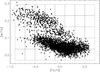 |
Fig. 1 Distribution of overall [Fe/H] and [α/Fe] for the APOGEE-TGAS sample (limited to σ(p) /p< 0.3) described in Sect. 3. |
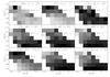 |
Fig. 2 Kinematics for the APOGEE-TGAS stars. The top panels show the average values in the boxes introduced in Fig. 1 for the Galactic velocity components UVW. The middle panels show the dispersion in the same velocities. The bottom panel shows the orbital elements: the guiding center (Rm), eccentricity (e), maximum distance from the Milky way plane (Zmax)). The grayscale is linear and spans the numerical ranges indicated in each panel from the minimum (black) to the maximum (white – just above the range of the data). |
Figure 1 shows the distribution of the sample in the [α/Fe]-[Fe/H] plane, and as in other samples, stars may be divided into two main populations, one with lower α/Fe abundance ratios and another with higher ratios, associated with the thin and thick components of the disk, respectively. As discussed in Sect. 1, some have argued that there is a distinct third group in-between these two, corresponding to stars with intermediate α/Fe abundance ratios, here evident at [Fe/H] ~ 0 and [α/Fe] ~ 0.12. Haywood (2013), Haywood et al. (2016) and Feuillet et al. (2016) show that that group of stars indeed shows intermediate ages between those in the lower and higher [α/Fe] sequences. However, that does not resolve the issue of whether they belong to a distinct third population.
To examine whether those stars should be associated with those with higher α/Fe ratios or not, we consider the stellar kinematics. We combined the TGAS astrometry and the APOGEE radial velocities to calculate the Galactic velocities of the stars with respect to the local standard of rest (LSR). We adopted for the solar motion relative to the LSR the values of Schönrich et al. (2010), (U, V, W)⊙ = (11.1,12.24,7.25), and followed the recipe described by Johnson & Soderblom (1987). The impact of the uncertainties in the astrometry on the derived Galactic velocities is modest, with mean (and standard deviation) of the uncertainties in V of 2 (2), 4 (4) and 6 (5) km s-1 for sub-samples defined according to the relative uncertainties in the parallax σ(p) /p = 0.1, 0.2 and 0.3, respectively, which is significantly less than the velocity spread of the disk.
The top panel of Fig. 2 shows the average radial (U), azimuthal (V), and vertical (W) velocity components for each of the boxes shown in Fig. 1, while the middle panels show the corresponding dispersions. A box size of 0.2 dex in [Fe/H] and 0.065 dex in [α/Fe] has been chosen as a trade-off between adequate statistical errors and our ability to sample variations in kinematics as a function of chemistry. It also gives us two average values for each of the main high-α and low-α populations at any given [Fe/H], which provides a consistency check. As anticipated from the discussion in Sect. 1, the most relevant quantities that allow a separation between the thin (low-α) and thick disk (high-α) components are the Galactic rotation (V), and the dispersion in all components (σU, σV and σW). Nevertheless, to the level we can say with these data, the boxes with intermediate values of [α/Fe] tend to have intermediate kinematics. There is even some marginal indication that the stars with intermediate α-to-iron ratios are kinematically closer to the thin disk than to the thick disk population.
We infer orbital parameters for all our chosen sample using our derived space velocities and galpy1 (Bovy 2015). The resulting mean orbital radius (Rm), eccentricities (e), and maximum height from the Galactic plane (Zmax) are shown in the bottom panel of Fig. 2. The average values for Rm and Zmax of the stars in the box at [Fe/H] ~ 0 and [α/Fe] ~ 0.12 have again intermediate values. The mixed values for the kinematics and orbital parameters of the stars with intermediate values of [alpha/Fe] are not due to confusion between the thin and thick disk populations, since the APOGEE statistical errors in [Fe/H] and [α/Fe] are about 0.01–0.03 dex.
We conclude that, at least with the APOGEE-TGAS data set, it is hard to decide whether the intermediate α stars are part of the thick disk or not. We conservatively take the approach of adopting as thin and thick disk stars only those with extreme [α/Fe] values: thin disk are taken as stars with [α/Fe] < 0.1 and thick disk stars as those with + 0.17 < [α/ Fe] < + 0.3. We measure the mean velocity and velocity dispersion for each population (see Table 1), and make use of the mean Galactic rotation velocities measured in each box to examine their dependence on stellar metallicity. This is illustrated in Fig. 3, where different symbols are used for individual stars, and mean values for the boxes. Similarly to Lee et al. (2011), Recio-Blanco et al. (2015), or Adibekyan et al. (2013), linear trends are apparent after binning. However, the scatter among individual stars in a given population is quite large, in particular for the thick disk.
The binned data are obtained by computing average values and their uncertainties, assuming a normal distribution ( ), in both axes. These data are fit with a linear relationship taking the uncertainties in both axes into account. The linear fittings indicate dV/ d [Fe/H] = −18 ± 2 km s-1 dex-1 for the thin disk, and dV/ d [Fe/H] = + 23 ± 10 km s-1 dex-1 for the thick disk. The value for the thin disk is of a very high significance, and in excellent agreement with previous results in the literature, e.g., −17 ± 4 km s-1 dex-1 by Adibekyan et al. (2013), or −17 ± 6 by Recio-Blanco et al. (2015), but slightly discrepant with −22 ± 3 by Lee et al. (2011). The result for the thick disk stars is more uncertain but points to a flatter V-[Fe/H] relation than those reported in previous studies, and is discussed below.
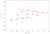 |
Fig. 3 Galactic rotation velocity derived for the APOGEE-TGAS (DR12) sample. Stars chemically associated with the thin and thick disks are shown as black and red dots, respectively. The average values found in the boxes introduced in Fig. 1 are shown as triangles, and the straight lines correspond to linear least-squares fits to the average values. The filled circles correspond to the intermediate-[α/Fe] stars not included in the thin or thick disk samples. The average values typically come in pairs at any given [Fe/H], since both the thin and thick disk populations are covered by two rows of boxes in Fig. 1. |
The average values for the stars that fall in boxes with intermediate 0.1 ≤ [α/ Fe] ≤ 0.17 ratios are shown with filled circles in Fig. 3. In addition to intermediate values for the α/Fe ratios, and intermediate metallicity and age distributions, these stars exhibit intermediate values for the Galactic rotation velocities and their dependence on [Fe/H].
Mean and standard deviation for the TGAS-APOGEE sample with uncertainties in parallax smaller than 30%.
The Hipparcos catalog, despite its small size, offers independent support for the results derived for the TGAS stars. There are 654 giant stars in common between Hipparcos and APOGEE – basically the sample described by Feuillet et al. (2016), obtained for validation of the results from the APOGEE pipeline. Adopting exactly the same criteria described for the TGAS-APOGEE sample, we arrive at dV/ d [Fe/H] = −10 ± 4 km s-1 dex-1 for the thin disk, and dV/ d [Fe/H] = +44 ± 44 km s-1 dex-1 for the thick disk. The slope for the thick disk is significantly more uncertain than the TGAS-APOGEE result, but consistent with them within the uncertainties. The thick disk gradient is shallower than in the TGAS-APOGEE sample.
The most recent data release of the SDSS, DR13 (Albareti et al. 2016), made public on July 2016, contains the same APOGEE stellar sample as DR12, but benefit from upgrades in the data and analysis pipelines. If we replace the DR12 abundances (which in the context of this paper are limited to [Fe/H] and [α/Fe]) by those in DR13 and repeat the analysis for the σ(p) /p < 0.3 TGAS sample, we arrive dV/ d [Fe/H] = −23 ± 2 km s-1 dex-1 for the thin disk, and dV/ d [Fe/H] = +33 ± 15 km s-1 dex-1 for the thick disk, which are statistically consistent with the results for DR12, but show that systematic erros associated with the metallicity scale can easily amount to ~5 km s-1 dex-1.
The uncertainties in the astrometry have a modest effect on the derived kinematics, and we have chosen to retain stars with relative uncertainties in the parallaxes better than 30%. Since the uncertainties in proper motion are tightly correlated with those in parallax, and both are tied to the stellar brightness, a simple limit in the parallax uncertainty involves a more general limit on the overall astrometric quality. If we were to enforce a more strict limit on the uncertainties, say 10% in relative parallax, the sample would be severely reduced to 547 stars. This will still provide a statistically robust result for the thin disk of dV/d[Fe/H] = –18 ± 5 km s-1 dex-1, but an inconclusive slope for the thick disk stars: dV/d[Fe/H] = + 21 ± 45 km s-1 dex-1. Similarly, retaining stars with relative parallax uncertainties under 20% will lead to dV/d[Fe/H] = –18 ± 2 km s-1 dex-1 and dV/d[Fe/H] = + 11 ± 13 km s-1 dex-1 for the thin and thick disks, respectively. However, if we relax the limits on the astrometric quality to enforce only a 40%, 50% or 100% parallax error, progressively increasing the sample size, the results remain robust, as reflected in Table 2. This weak dependence of our results on the astrometric uncertainties is the result of the increase in sample size associated with imposing more relaxed limits, and the fact that a large fraction of the sample concentrates towards l = 90 and b = 0 – about 1/3 of the stars are within 30 degrees from that direction – mainly due to the extensive APOGEE program to follow-up Kepler stars (APOKASC; see Pinsonneault et al. 2015).
It is apparent that the average rotation velocity for stars in the boxes centered at [Fe/H] = −0.6 and −0.4 (squares at those values in Fig. 3) may split in two groups, one with high and one with low V velocity. We observe that the larger V velocities correspond to the boxes with the highest [α/Fe] values (those centered at [α/Fe] = + 0.26). This is in line with the findings by Recio-Blanco et al. (2015), who found a steeper positive value for dV/d[Fe/H] for thick disk stars with lower [α/Fe] ratios.
Mean dV/d[Fe/H] values derived for the thin disk ([α/Fe] < 0.1) and thick disk ([α/Fe] > 0.17) stars for subsamples defined by an upper limit to the relative uncertainty in the relative Gaia TGAS parallaxes.
Biases may arise because stars with intermediate [α/Fe] abundance ratios show intermediate kinematics between the high-α ([α/Fe] > 0.18) and the low-α populations. It is easy to see by inspection of Fig. 3 that including the stars with intermediate [α/Fe] and relatively higher [Fe/H] will enhance the derived dV/d[Fe/H] gradient for the thick disk population. In addition, as mentioned in Sect. 1, halo stars are more likely to enter in the low-metallicity side of the thick disk distribution, which can lead to an artificially steeper slope. This issue might already be mildly affecting our analysis, since capping the thick disk TGAS sample to V> −100 km s-1 would slightly flatten our slope for this population from dV/d[Fe/H] = + 23 ± 10 to dV/d[Fe/H] = + 14 ± 9, but we stress that such a limit in V would be certainly extreme.
Our data permit a fairly reliable determination of the correlation between orbital eccentricity and metallicity for each sub-sample. Here, eccentricity is calculated from the orbital apocenter and pericenter as e = (Rapo−Rperi)/(Rapo + Rperi). For the thin disk stars we find de/d[Fe/H] = −0.05 ± 0.01 dex-1, while for the thick disk sample we find de/d[Fe/H] = −0.11 ± 0.03 dex-1. These results are consistent with the measurements reported by Adibekyan et al. (2013), de/d[Fe/H] =−0.023 ± 0.015 dex-1 for the thin disk stars and de/d[Fe/H] = −0.184 ± 0.078 dex-1 for the thick disk stars. We note that Adibekyan et al. include disk candidate stars down to [Fe/H] ≃ −1.4, a domain in which it becomes difficult to eliminate halo stars from local samples, which could produce a pronounced increase in the eccentricity of the metal-poor stars in the sample.
We need d[Fe/H]/de for a convenient parameterization in the models described below, and since there is significant scatter in the [Fe/H]-e relation, the best fit d[Fe/H]/de does not equal 1/(de/d[Fe/H]). We measure d[Fe/H]/de = −0.34 ± 0.08 for the thick disk stars in the TGAS-APOGEE sample.
4. Model comparison
To understand the observed dV/d[Fe/H] trend for the thick and thin disk populations, we compare our results with a snapshot of an N-body simulation. The N-body simulation model used is the same as Model A of Kawata et al. (2016), but with a different initial velocity dispersion for the thick disk particles, with  instead of
  for Model A, since this leads to a more realistic ratio between the azimuthal and vertical velocity dispersions. We use our Tree N-body code, GCD+ (Kawata & Gibson 2003; Kawata et al. 2013) for the N-body simulation.
We initially set up an isolated disk galaxy which consists of stellar thick and thin exponential disks, with no bulge component, in a static Navarro et al. (1997) dark matter halo potential (Rahimi & Kawata 2012; Grand et al. 2012). The initial scale length and scale heights of thick (thin) disks are set to be Rd,thick = 2.5 kpc (Rd,thin = 4.0 kpc) and zd,thick = 1.0 kpc (zd,thin = 0.35 kpc), respectively. The mass of the thick and thin disks are Md,thin = 4.5 × 10¹⁰M⊙ and Md,thick = 1.5 × 10¹⁰M⊙.
We used a snapshot at t = 1 Gyr, after spiral arms have developed, but before a bar forms. The model is a pure N-body simulation, and there is no gas component or growth of the stellar disk for simplicity. We chose this particular snapshot because the azimuthal, σV, and vertical, σW, velocity dispersions for the thin and thick disk at the Solar radius are similar to those observed in the Milky Way. Unfortunately, we do not have an N-body simulation having all three components of the velocity dispersion consistent with the Milky Way disk. We prioritized σV and σW, and compromised on σU.
We tagged the particles belonging to the thin disk component at the start of the simulation. From our TGAS-APOGEE sample, we measured the radial metallicity gradient as a function of mean orbital Galactocentric radius, Rm, and the vertical gradient as a function of Zmax, and found d[Fe/H]/dRm = −0.053 ± 0.004 dex kpc-1 and d[Fe/H]/dZmax = −0.34 ± 0.03 dex kpc-1. We then assigned metallicities to the particles, according to their Galactocentric distances, [Fe/H] = −0.05 × Rm−0.3 × | Z | + 0.4 dex, with a dispersion of 0.2 dex, where Rm = (Rapo + Rperi)/2 is the mean radius of the orbit, Rapo and Rperi are the particle’s apo- and pericenter radii, respectively, and | Z | is the current vertical height. We ran a test particle simulation for the selected particles under the gravitational potential calculated from the frozen particle distribution, and analyzed Rapo and Rperi. Note that we used the current vertical height instead of Zmax for simplicity.
We selected particles within a ring at 7.5 <R< 8.5 kpc and | Z | < 0.5 kpc to mimic a volume roughly consistent with that occupied by our TGAS-APOGEE stars, assuming that the Galactocentric radius of the Sun is 8 kpc. The velocity dispersion of the selected sample of particles is (σU,σV,σW) = (28,22,18) km s-1. As mentioned above, the radial velocity dispersion, σU, is smaller than the observed σU of the thin disk population of the Milky Way (see our TGAS-APOGEE results in Table 1). Figure 4 shows the rotation velocity, V, and [Fe/H] of the selected particles, where metallicity has been assigned with the above formula. The figure includes the mean values and the dispersion for the binned data as a function of [Fe/H], and the line of best fit, corresponding to dV/d[Fe/H] = −16.9 ± 0.2 km s-1 kpc-1. The inferred dV/d[Fe/H] is qualitatively consistent with what we observed for the thin disk stars in Sect. 3. Our only assumptions were negative radial and vertical metallicity gradients. We tested and found that assuming a zero vertical metallicity gradient does not change the slope of the derived V-[Fe/H] relationship. Therefore, the negative value of dV/d[Fe/H] is mainly driven by the negative radial metallicity gradient.
Because of the epicyclic motion of the stars, stars moving with a larger azimuthal velocity in the Solar neighborhood tend to be close to their pericenter phase, meaning that their guiding center is larger than the Solar radius and therefore they tend to come from outer radii. Conversely, stars rotating slower preferentially have a guiding center smaller than the solar radius. Hence, if there is a negative metallicity gradient as a function of the guiding center or the mean radius, Rm this trend can drive a negative slope in the V-[Fe/H] relation (see also Vera-Ciro et al. 2014).
From this simple model, we can say that the observed negative slope in the V-[Fe/H] relation can be simply explained by the epicyclic motion of stars, given the observed radial metallicity gradient. Although it is often mentioned that the negative value of dV/d[Fe/H] for thin disk stars is an evidence of radial migration, it can be explained solely by the epicyclic motion (blurring), and does not require changes of angular momentum of the stars (churning, see Sellwood et al. 2002 ).
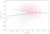 |
Fig. 4 Galactic rotation velocity derived for the particles in the simulations for the thin (red) and thick disk (black). The particle’s velocities are treated similarly as the observed stars described in Sect. 3, and only one in ten particles are shown in the figure. The linear fittings give dV/d[Fe/H] = −16.9 ± 0.2 km s-1 (thin disk) and dV/d[Fe/H] = + 16 ± 1 km s-1 (thick disk). |
We then analyzed the V-[Fe/H] relation for particles that are initially assigned to the thick disk population in a similar way. The thick disk population of the Milky Way shows a flat radial metallicity gradient, but a negative vertical metallicity gradient approximately d[Fe/H] /dZ = −0.1 (Mikolaitis et al. 2014; Hayden et al. 2015).
As discussed in Sect. 3, the chemically defined thick disk stars have a correlation between [Fe/H] and orbital eccentricity, e, with higher e stars having lower [Fe/H]. Hence we assigned metallicity to the thick disk particles following the relationship [Fe/H] = −0.35 × (e−0.2)−0.1 × | Z | −0.01 × Rm−0.2 dex with a dispersion of 0.175 dex.
We found that the negative value of d[Fe/H]/de leads to a slight positive radial metallicity gradient, because the velocity dispersion decreases with Galactocentric distance, and therefore the stars with a smaller guiding center tend to have higher eccentricity. Hence, we applied a shallow negative radial metallicity gradient, to make the overall radial metallicity gradient flat as observed (Bensby et al. 2011; Mikolaitis et al. 2014; Hayden et al. 2015). We have checked that the metallicity distributions of this model match well with the metallicity distribution function at the different radii and vertical heights of [α/Fe] > 0.17 dex stars in the APOGEE DR12 data (Hayden et al. 2014, 2015).
Again, we selected the thick disk particles within a ring at 7.5 <R< 8.5 kpc and | Z | < 0.5 kpc. The velocity dispersion of the selected sample of particles is (σR,σφ,σz) = (40,34,39) km s-1. Although σφ and σz are consistent with the observed velocity dispersions, the radial velocity dispersion, σR, is significantly smaller than the observed σR for the thick disk population. The V-[Fe/H] relation for thick disk particles is shown in Fig. 4. The mean values after binning the data as in our analysis of the TGAS-APOGEE data are also shown, and so is the best linear fit. A positive slope dV/d[Fe/H] = 16 ± 1 km s-1 dex-1 is found for this simple model, qualitatively consistent with the observed positive slope for the thick disk stars in our TGAS-APOGEE sample. The positive dV/d[Fe/H] of this model is driven by the assumed eccentricity-metallicity relation, lower metallicity stars having orbits with a higher eccentricity and therefore a slower mean rotation velocity. This trend can be interpreted in a scenario in which the thick disk initially formed from lower metallicity and kinematically hotter gas disk, and gradually became more metal rich and kinematically colder, perhaps due to more gas-rich minor mergers at a higher redshift, as expected due to hierarchical clustering (e.g., Brook et al. 2004, 2012).
Another way of creating a steep positive dV/d[Fe/H] is applying a positive radial metallicity gradient with Rm (Curir et al. 2012). This would need to have the opposite slope to that we adopted for the thin disk particles. For the same reason given for the thin disk particles, a positive d[Fe/H]/dRm can drive a positive dVφ/ d [Fe/H]. However, this model disagrees with the observed flat radial metallicity gradient and the negative vertical metallicity gradient of the thick disk of the Milky Way.
Our simple model is sufficient to support a qualitative discussion whether or not a simple metallicity distribution difference can explain the observed trends of dV/d[Fe/H] for the thick and thin disk populations. Fine tuning of our model to quantitatively match the observational data, or to provide a unique solution, is beyond the scope of this paper. Still, this comparison highlights that the measurement of dV/d[Fe/H] provides strong constraints on the kinematical and chemical properties of the thick and thin disks.
5. Summary
Combining astrometric information from the Gaia’s first data release and chemical abundances from the SDSS APOGEE survey, we measured the Galactic rotation velocity-[Fe/H] relation for the thick and thin disk stars identified on the basis of their [α/Fe] abundance ratio. We selected the sample of stars common to the two surveys with strict criteria of relative parallax errors less than 0.3, a specific log g and Teff range to select giant stars (for which the APOGEE abundances are more reliable), and [Fe/H] > −1.0 to minimize contamination from halo stars. We also defined the thick and thin disk more strictly by requiring [α/Fe] < 0.1 dex and 0.17 < [α/Fe], respectively. We find that dV/d[Fe/H] = −18 ± 2 km s-1 dex-1 for thin disk stars and dV/d[Fe/H] = + 23 ± 10 km s-1 dex-1 for thick disk stars. We therefore confirm that the slope of the V-[Fe/H] relationship is different for the thin and thick disks. The negative dV/d[Fe/H] for thin disk stars is consistent with previous studies. However, our measurement of dV/d[Fe/H] for thick disk stars is flatter than what is claimed in previous studies. In addition, we find evidence that dV/d[Fe/H] depends on [α/Fe] for thick disk stars.
Stars with intermediate [α/Fe] values are known to exhibit intermediate ages, metallicity distributions, and kinematics. We find that they show an approximately flat variation of the V-[Fe/H] relation, that is, an intermediate slope between the negative value for the thin disk and the positive one for the thick disk.
Using a simple N-body model, we demonstrate that the observed negative dV/d[Fe/H] for the thin disk can be explained by the observed negative metallicity gradient as a function of the mean orbital radius. The negative dV/d[Fe/H] can be explained solely by the epicyclic motion of the stars (blurring), and it is not an evidence of radial migration with the change in angular momentum and guiding radius (churning). Our simple N-body model also demonstrates that the positive value of dV/d[Fe/H] for the thick disk can be naturally explained with the observed [Fe/H]-eccentricity correlation, with stars with higher eccentricity having lower [Fe/H]. This model provides a satisfactory explanation for the different signs of the slope of the V-[Fe/H] relationship for the thin and thick disks.
Our TGAS-APOGEE results indicate that the negative slope of the V-[Fe/H] relation for the thin disk is robustly measured. However, dV/d[Fe/H] for the thick disk is sensitive to how the thick disk population is defined. Larger samples of stars with sufficient accuracy in their astrometric measurements and associated chemistry are required to disentangle the correlations between kinematics and abundances in the thick disk. This study highlights the synergy between astrometric data from Gaia and high-resolution spectroscopy. Future Gaia data releases and ongoing ground-based spectroscopic surveys will further refine the measurements of the V-[Fe/H] relation for thick and thin disks, and at the same time will allow us to measure the chemodynamical signatures of the different stellar populations, not only in the solar neighborhood, but also over a wide range of the Galactic disk, providing strong constraints on the formation of the thick and thin disks of the Milky Way.
Acknowledgments
We thank our colleagues, in particular Ignacio Ferreras and George Seabroke, for enlightening discussions, an anonymous referee for suggestions, and Ron Drimmel for pointing out a missing important reference. C.A.P. is grateful for support from MINECO for this research through grant AYA2014-56359-P, and to the Severo Ochoa Excellence program for funding his visit to MSSL in Summer 2016. D.K. and M.C. gratefully acknowledge the support of the UK’s Science & Technology Facilities Council (STFC Grant ST/K000977/1 and ST/N000811/1). The numerical Galaxy models for this paper were simulated on the UCL facility Grace, and the DiRAC Facilities (through the COSMOS and MSSL-Astro consortium) jointly funded by STFC and the Large Facilities Capital Fund of BIS. We also acknowledge PRACE for awarding us access to their Tier-1 facilities. This work has made use of data from the European Space Agency (ESA) mission Gaia2, processed by the Gaia Data Processing and Analysis Consortium (DPAC3). Funding for the DPAC has been provided by national institutions, in particular the institutions participating in the Gaia Multilateral Agreement. Funding for the Sloan Digital Sky Survey IV has been provided by the Alfred P. Sloan Foundation, the U.S. Department of Energy Office of Science, and the Participating Institutions. SDSS acknowledges support and resources from the Center for High-Performance Computing at the University of Utah. The SDSS web site is www.sdss.org. SDSS is managed by the Astrophysical Research Consortium for the Participating Institutions of the SDSS Collaboration including the Brazilian Participation Group, the Carnegie Institution for Science, Carnegie Mellon University, the Chilean Participation Group, the French Participation Group, Harvard-Smithsonian Center for Astrophysics, Instituto de Astrofísica de Canarias, The Johns Hopkins University, Kavli Institute for the Physics and Mathematics of the Universe (IPMU)/University of Tokyo, Lawrence Berkeley National Laboratory, Leibniz Institut für Astrophysik Potsdam (AIP), Max-Planck-Institut für Astronomie (MPIA Heidelberg), Max-Planck-Institut für Astrophysik (MPA Garching), Max-Planck-Institut für Extraterrestrische Physik (MPE), National Astronomical Observatory of China, New Mexico State University, New York University, University of Notre Dame, Observatorio Nacional/MCTI, The Ohio State University, Pennsylvania State University, Shanghai Astronomical Observatory, United Kingdom Participation Group, Universidad Nacional Autónoma de México, University of Arizona, University of Colorado Boulder, University of Oxford, University of Portsmouth, University of Utah, University of Virginia, University of Washington, University of Wisconsin, Vanderbilt University, and Yale University.
References
- Adibekyan, V. Zh., Figueira, P., Santos, N. C., et al. 2013, A&A, 554, A44 [NASA ADS] [CrossRef] [EDP Sciences] [Google Scholar]
- Alam, S., Albareti, F. D., Allen de Prieto, C., et al. 2015, ApJS, 219, 1 [NASA ADS] [CrossRef] [Google Scholar]
- Albareti, F. D., Allende Prieto, C., et al. 2016, ApJS, submitted [arXiv:1608.02013] [Google Scholar]
- Anders, F., Chiappini, C., Santiago, B. X., et al. 2014, A&A, 564, A115 [NASA ADS] [CrossRef] [EDP Sciences] [Google Scholar]
- Bensby, T., Alves-Brito, A., Oey, M. S., Yong, D., & Meléndez, J. 2011, ApJ, 735, L46 [NASA ADS] [CrossRef] [Google Scholar]
- Bensby, T., Feltzing, S., & Oey, M. S. 2014, A&A, 562, A71 [NASA ADS] [CrossRef] [EDP Sciences] [Google Scholar]
- Bertran de Lis, S., Allende Prieto, C., Majewski, S. R., et al. 2016, A&A, 590, A74 [NASA ADS] [CrossRef] [EDP Sciences] [Google Scholar]
- Bond, N. A., Ivezić, Ž., Sesar, B., et al. 2010, ApJ, 716, 1 [NASA ADS] [CrossRef] [Google Scholar]
- Bovy, J. 2015, ApJS, 216, 29 [NASA ADS] [CrossRef] [Google Scholar]
- Bovy, J., Rix, H.-W., & Hogg, D. W. 2012, ApJ, 751, 131 [NASA ADS] [CrossRef] [Google Scholar]
- Brook, C. B., Kawata, D., Gibson, B. K., & Freeman, K. C. 2004, ApJ, 612, 894 [NASA ADS] [CrossRef] [Google Scholar]
- Brook, C. B., Stinson, G. S., Gibson, B. K., et al. 2012, MNRAS, 426, 690 [NASA ADS] [CrossRef] [Google Scholar]
- Curir, A., Lattanzi, M. G., Spagna, A., et al. 2012, A&A, 545, A133 [NASA ADS] [CrossRef] [EDP Sciences] [Google Scholar]
- Eisenstein, D. J., Weinberg, D. H., Agol, E., et al. 2011, AJ, 142, 72 [Google Scholar]
- Fuhrmann, K. 2011, MNRAS, 414, 2893 [NASA ADS] [CrossRef] [Google Scholar]
- Gaia Collaboration (Prusti, T., et al.) 2016a, A&A, 595, A1 [NASA ADS] [CrossRef] [EDP Sciences] [Google Scholar]
- Gaia Collaboration (Brown, A. C. A., et al.) 2016b, A&A, 595, A2 [NASA ADS] [CrossRef] [EDP Sciences] [Google Scholar]
- García Pérez, A. E., Allende Prieto, C., Holtzman, J. A., et al. 2016, AJ, 151, 144 [NASA ADS] [CrossRef] [Google Scholar]
- Gilmore, G., Randich, S., Asplund, M., et al. 2012, The Messenger, 147, 25 [NASA ADS] [Google Scholar]
- Grand, R. J. J., Kawata, D., & Cropper, M. 2012, MNRAS, 421, 1529 [CrossRef] [Google Scholar]
- Hayden, M. R., Holtzman, J. A., Bovy, J., et al. 2014, AJ, 147, 116 [NASA ADS] [CrossRef] [MathSciNet] [Google Scholar]
- Hayden, M. R., Bovy, Jo, Holtzman, J. A., et al. 2015, ApJ, 808, 132 [NASA ADS] [CrossRef] [Google Scholar]
- Holtzman, J. A., Shetrone, M., Johnson, J. A., et al. 2015, AJ, 150, 148 [NASA ADS] [CrossRef] [Google Scholar]
- Ivezić, Ž., Sesar, B., Jurić, M., et al. 2008, ApJ, 684, 287 [NASA ADS] [CrossRef] [Google Scholar]
- Johnson, D. R. H., & Soderblom, D. R. 1987, AJ, 93, 864 [NASA ADS] [CrossRef] [Google Scholar]
- Kawata, D., & Gibson, B. K. 2003, MNRAS, 340, 908 [Google Scholar]
- Kawata, D., Okamoto, T., Gibson, B. K., Barnes, D. J., & Cen, R. 2013, MNRAS, 428, 1968 [NASA ADS] [CrossRef] [Google Scholar]
- Kawata, D., Grand, R. J. J., Gibson, B. K., et al. 2016, MNRAS, 464, 702 [Google Scholar]
- Lee, Y. S., Beers, T. C., An, D., et al. 2011, ApJ, 738, 187 [NASA ADS] [CrossRef] [Google Scholar]
- Lindegren, L., Lammers, U., Bastian, U., et al. 2016, A&A, 595, A4 [NASA ADS] [CrossRef] [EDP Sciences] [Google Scholar]
- Majewski, S. R., Schiavon, R. P., Frinchaboy, P. M., et al. 2016, AJ, submitted [arXiv:1509.05420] [Google Scholar]
- Mikolaitis, Š., Hill, V., Recio-Blanco, A., et al. 2014, A&A, 572, A33 [NASA ADS] [CrossRef] [EDP Sciences] [Google Scholar]
- Navarro, J. F., Frenk, C. S., & White, S. D. M. 1997, ApJ, 490, 493 [NASA ADS] [CrossRef] [Google Scholar]
- Rahimi, A., & Kawata, D. 2012, MNRAS, 422, 2609 [NASA ADS] [CrossRef] [Google Scholar]
- Ramírez, I., Allende Prieto, C., & Lambert, D. L. 2013, ApJ, 764, 78 [NASA ADS] [CrossRef] [Google Scholar]
- Recio-Blanco, A., de Laverny, P., Kordopatis, G., et al. 2014, A&A, 567, A5 [NASA ADS] [CrossRef] [EDP Sciences] [Google Scholar]
- Vera-Ciro, C., D’Onghia, E., Navarro, J., & Abadi, M. 2014, MNRAS, 794, 173 [Google Scholar]
- Sellwood, J. A., & Binney, J. J. 2002, MNRAS, 336, 785 [NASA ADS] [CrossRef] [Google Scholar]
- Spagna, A., Lattanzi, M. G., Re Fiorentin, P., & Smart, R. L. 2010, A&A, 510, L4 [NASA ADS] [CrossRef] [EDP Sciences] [Google Scholar]
All Tables
Mean and standard deviation for the TGAS-APOGEE sample with uncertainties in parallax smaller than 30%.
Mean dV/d[Fe/H] values derived for the thin disk ([α/Fe] < 0.1) and thick disk ([α/Fe] > 0.17) stars for subsamples defined by an upper limit to the relative uncertainty in the relative Gaia TGAS parallaxes.
All Figures
|
Fig. 1 Distribution of overall [Fe/H] and [α/Fe] for the APOGEE-TGAS sample (limited to σ(p) /p< 0.3) described in Sect. 3. |
| In the text | |
|
Fig. 2 Kinematics for the APOGEE-TGAS stars. The top panels show the average values in the boxes introduced in Fig. 1 for the Galactic velocity components UVW. The middle panels show the dispersion in the same velocities. The bottom panel shows the orbital elements: the guiding center (Rm), eccentricity (e), maximum distance from the Milky way plane (Zmax)). The grayscale is linear and spans the numerical ranges indicated in each panel from the minimum (black) to the maximum (white – just above the range of the data). |
| In the text | |
|
Fig. 3 Galactic rotation velocity derived for the APOGEE-TGAS (DR12) sample. Stars chemically associated with the thin and thick disks are shown as black and red dots, respectively. The average values found in the boxes introduced in Fig. 1 are shown as triangles, and the straight lines correspond to linear least-squares fits to the average values. The filled circles correspond to the intermediate-[α/Fe] stars not included in the thin or thick disk samples. The average values typically come in pairs at any given [Fe/H], since both the thin and thick disk populations are covered by two rows of boxes in Fig. 1. |
| In the text | |
|
Fig. 4 Galactic rotation velocity derived for the particles in the simulations for the thin (red) and thick disk (black). The particle’s velocities are treated similarly as the observed stars described in Sect. 3, and only one in ten particles are shown in the figure. The linear fittings give dV/d[Fe/H] = −16.9 ± 0.2 km s-1 (thin disk) and dV/d[Fe/H] = + 16 ± 1 km s-1 (thick disk). |
| In the text | |
Current usage metrics show cumulative count of Article Views (full-text article views including HTML views, PDF and ePub downloads, according to the available data) and Abstracts Views on Vision4Press platform.
Data correspond to usage on the plateform after 2015. The current usage metrics is available 48-96 hours after online publication and is updated daily on week days.
Initial download of the metrics may take a while.