| Issue |
A&A
Volume 596, December 2016
|
|
|---|---|---|
| Article Number | A95 | |
| Number of page(s) | 13 | |
| Section | Extragalactic astronomy | |
| DOI | https://doi.org/10.1051/0004-6361/201629343 | |
| Published online | 09 December 2016 | |
Spectral nuclear properties of NLS1 galaxies⋆
1 Instituto de Astronomía Teórica y
Experimental (IATE), Universidad Nacional de Córdoba, CONICET, Observatorio
Astronómico de Córdoba, Laprida
854, Córdoba, Argentina
e-mail: This email address is being protected from spambots. You need JavaScript enabled to view it.
2 Observatorio Astronómico, Universidad
Nacional de Córdoba, Laprida
854, 5000
Córdoba,
Argentina
Received:
19
July
2016
Accepted:
4
August
2016
Abstract
Context. It is not yet well known whether narrow line Seyfert 1 (NLS1) galaxies follow the MBH − σ⋆ relation found for normal galaxies. Emission lines, such as [SII] or [OIII]λ5007, have been used as a surrogate of the stellar velocity dispersion and various results have been obtained. On the other hand, some active galactic nuclei (AGNs) have shown Balmer emission with an additional intermediate component (IC) besides the well-known narrow and broad lines. The properties of this IC have not yet been fully studied.
Aims. In order to re-examine the location of NLS1 in the MBH − σ⋆ relation, we test some emission lines, such as the narrow component (NC) of Hα and the forbidden [NII]λλ6548,6584 and [SII]λλ6716,6731 lines, as replacements for σ⋆. On the other hand, we study the properties of the IC of Hα found in 14 galaxies of the sample to find a link between this component, the central engine, and the remaining lines. We also compare the emission among the broad component (BC) of Hα and those emitted at the narrow line region (NLR) to detect differences in the ionizing source in each emitting region.
Methods. We have obtained and studied medium-resolution spectra (170 km s-1 FWHM at Hα) of 36 NLS1 galaxies in the optical range ~5800−6800 Å. We performed a Gaussian decomposition of the Hα +[NII]λλ6548,6584 profile to study the distinct components of Hα and [NII] lines. We also measured the [SII] lines.
Results. We obtained black hole (BH) masses in the range log (MBH/M⊙) = 5.4−7.5 for our sample. We found that, in general, most of the galaxies lie below the MBH − σ⋆ relation when the NC of Hα and [NII] lines are used as a surrogate of σ⋆. The objects are closer to the relation when [SII] lines are used. Nevertheless, the galaxies are still below this relation and we do not see a clear correlation between the BH masses and FWHM[SII]. Besides this, we found that 13 galaxies show an IC, most of which are in the velocity range ~700−1500 km s-1. This is same range as in AGN types and is well correlated with the FWHM of BC and, therefore, with the BH mass. On the other hand, we found that there is a correlation between the luminosity of the BC of Hα and NC, IC, [NII]λ6584, and [SII] lines.
Key words: galaxies: active / galaxies: Seyfert / galaxies: nuclei / galaxies: kinematics and dynamics
The reduced spectra as FITS files are only available at the CDS via anonymous ftp to cdsarc.u-strasbg.fr (130.79.128.5) or via http://cdsarc.u-strasbg.fr/viz-bin/qcat?J/A+A/596/A95
Visiting Astronomer, Complejo Astronómico El Leoncito operated under agreement between the Consejo Nacional de Investigaciones Científicas y Técnicas de la República Argentina and the National Universities of La Plata, Córdoba, and San Juan.
© ESO, 2016
1. Introduction
Narrow line Seyfert 1 galaxies are a subclass of active galactic nuclei (AGNs). The most common defining criterion for these objects is the width of the broad component of their optical Balmer emission lines in combination with the relative weakness of the [OIII]λ5007 emission with full width half maximum (FWHM) ≤ 2000 km s-1 and the relative weakness of [OIII]λ5007/Hβ ≤ 3 (Osterbrock & Pogge 1985; Goodrich 1989). Optical spectroscopy classifications suggest that NLS1 represent about 15% of the whole population of Seyfert 1 galaxies (Williams et al. 2002).
Observations of NLS1, as well as other AGNs, clearly show different types of emission lines in their spectra. Depending on the width of the emitted lines, they are classified as narrow lines with FWHM of a few hundred of km s-1, or broad lines, with FWHM of a few thousand km s-1. This implies two different regions of line formation, i.e, narrow line region (NLR) and the broad line region (BLR), respectively.
In the middle of the ’90s various works on QSOs suggested that the traditional broad line region (BLR) consists of two components: one component with a FWHM of ~2000 km s-1, called the intermediate line region (ILR), and another very broad component (VBLR) with a FWHM of ~7000 km s-1 blueshifted by ≥1000 km s-1 (Brotherton et al. 1994; Corbin & Francis 1994). Brotherton suggested that the intermediate line region (ILR) arises in a region inner to the narrow line region (NLR). Mason et al. (1996) examined the profiles of Hα, Hβ, and [OIII] lines and found evidence for an intermediate-velocity (FWHM ≤ 1000 km s-1), line-emitting region that produces significant amounts of both permitted and forbidden lines. Crenshaw & Kraemer (2007) identified a line emission component with width FWHM = 1170 km s-1 for the Sy1 NGC 4151, most probably originating between the BLR and NLR. Hu et al. (2008) reported evidence for an intermediate line region in a sample of 568 quasar selected from the Sloan Digital Sky Survey (SDSS). They investigated the Hβ and FeII emission lines and observed that the conventional broad Hβ emission line could be decomposed into two components: one component with a very broad FWHM and the another with an intermediate FWHM. This ILR, whose kinematics seems to be dominated by infall, could be located in the outskirts of the BLR. In addition, Crenshaw et al. (2009) detected ILR emission with width of 680 km s-1 in the spectrum of NGC 5548. Mao et al. (2010) studied a sample of 211 narrow line Seyfert 1 galaxies selected from the SDSS, finding that the Hβ profile can be fitted well by three (narrow, intermediate, and broad) Gaussian components with a ratio FWHMBC/FWHMIC ~ 3 for the entire sample. Also, they suggested that the intermediate components originate from the inner edge of the torus, which is scaled by dust K-band reverberation. Related to this, there are some questions about the ILR. Is it linked to the central engine of the AGN? How is it related to the BLR emission? One of the aims of this paper is to answer these questions studying the intermediate component of Hα in NLS1 galaxies.
On the other hand, and related to the central dynamics, according to several authors there is a correlation between the BH masses and the velocity dispersion of the stars of the bulge of the host galaxy (e.g., Ferrarese & Merritt 2000; Gebhardt et al. 2000; Tremaine et al. 2002). Because of the difficulty of measuring the stellar velocity dispersion in AGNs, sometimes emission lines are used as a surrogate. For example, in the case of the [OIII]λ5007 line, various authors found that NLS1 are off the MBH − σ⋆ relation (e.g., Mathur et al. 2001; Bian & Zhao 2004; Grupe & Mathur 2004; Mathur & Grupe 2005a,b; Zhou et al. 2006) and on the contrary, other researchers found that these galaxies are on the relation (Wang & Lu 2001; Botte et al. 2005). Komossa & Xu (2007) found that using [SII] lines as a replacement for the stellar velocity dispersion, NLS1 galaxies are on the relation. In this paper we re-examine the location of the NLS1 galaxies in the MBH − σ⋆ relation using the narrow component of Hα (originated in the NLR) and the forbidden emission lines [NII] and [SII] as surrogates of stellar velocity dispersion.
As a whole, NLS1 galaxies represent a very interesting class of objects, and it is important to study them both from their structural and dynamical point of view and investigate how these objects fit into the unification schemes for AGNs. In order to study the intermediate component of Hα and to test various emission lines as a replacement for σ⋆ we studied 36 NLS1 galaxies, of which 27 are in the Southern Hemisphere. We carried out a spectroscopic study of these galaxies to analyze their internal kinematics and to derive properties regarding their BLR, NLR, and ILR. In Sect. 2 we present the sample and observations; a description of how the measurements were carried out is detailed in Sect. 3; in Sect. 4 we present the results regarding the nuclear dynamics, for example, the BH masses of the sample, location of the galaxies in the MBH − σ⋆ relation, and the intermediate component of Hα; and in Sect. 5 we show how the luminosities of the different lines are related. We present some curious individual cases in Sect. 6 and in Sect. 7 we draw our conclusions. Throughout this paper, we use the cosmological parameters H0 = 70 km s-1 Mpc-1, ΩM = 0.3, and ΩΛ = 0.7.
2. Observational data
2.1. Sample and observations
We have selected NLS1 galaxies from the Véron & Véron catalog (Véron-Cetty & Véron 2010) with redshifts z< 0.15 and brighter than mb< 18 with δ ≤ 10°. Of those objects, we chose galaxies whose nuclear kinematics are poorly or even not studied. This way our sample consists of 36 galaxies, of which 27 are in the Southern Hemisphere, while the remaining have 0°<δ ≤ 10°. This coordinate range allows us to observe the sample from the Complejo AStronómico el LEOncito (CASLEO), in Argentina.
Observations were performed in different campaigns between 2011 and 2014. We carried out long-slit spectroscopy using the REOSC spectrograph at CASLEO 2.15 m Ritchey-Chrétien telescope, San Juan, Argentina. The spectrograph has a Tektronix 1024 × 1024 CCD attached with 24 μm pixels. The galaxies were observed using a 2.7 arcsec wide slit and the extractions of each spectrum were of ~2.3 arcsec. For a mean distance of 240 Mpc (mean redshift of ~0.06) the spectra correspond to the central ~3 kpc in projected distance. We used a 600 line mm-1 grating giving a resolution of 170 km s-1 FWHM around Hα. The observations cover the spectral range from 5800 Å to 6800 Å. The spectra were calibrated in wavelengths using comparison lines from a Cu-Ne-Ar lamp and three standard stars were observed each night to flux calibrate the spectra. Standard data reduction techniques were used to process the data, mainly ccdred and longslit packages included in IRAF1. The obtained spectra have a mean signal to noise of ~16 around 6000 Å. Although some galaxies in our sample already have spectra, in most cases they have a lower resolution or are not flux calibrated (as in the cases of 2df and 6df spectra). In our sample, 11 objects have SDSS spectra with a very similar resolution. They were taken with the SDSS spectrograph, which has a fiber diameter of 3 arcsec. Table A.1 lists the galaxy name, right ascension, declination, apparent B magnitude, redshift, date of the observation, and exposure time.
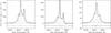 |
Fig. 1 From left to right: Gaussian decomposition for the galaxies MCG04.24.017, 2MASXJ05014863−2253232, and 2MASX J21124490− 3730119, respectively. Thick line represents the spectra; the Hα components and [NII]λ6548,6584 are shown in dotted lines. The residuals are plotted at the bottom of each panel and were displaced from zero for clarity. |
2.2. NLS1 spectra
Here we present the spectra of 36 NLS1s for the red spectral region 5800−6800 Å. In this work we focus on this spectral region to study in detail the emission lines such as Hα +[NII]λλ6548 6584 and [SII]λλ6716 6731.
The beginning of the spectral region presented conforms to the higher initial wavelength for the red observations, while there were usually sky absorption lines near 7000 Å. This made the measurement of sulfur lines difficult and, depending on the redshift, in many cases prevented these measurements, thus making 5800−6800 Å a compromise between these constrains.
Figure A.1 presents the spectra of the NLS1s for the red spectral region. All spectra are in rest frame for which we used the published redshift data from the NASA/IPAC Extragalactic Database (NED), and we present their fluxes in units of 10-17 erg cm-2 s-1 Å-1. As expected from photoionized gas in active nuclei, Hα +[NII] emission lines are the most important feature in all the objects, while in 25 out of 36 spectra [SII]λλ6716, 6731 lines are easily detected. We also identify [OI]λ6300 (over 3σ) in only seven objects. Sodium lines Naλλ5890, 5896 were detected, although these (as well as other absorption lines) are often weak mainly because of the dilution of the stellar features by a nonstellar continuum; these lines also appear in emission in some cases.
3. Emission line measurements
Our interest resides in the emission lines, which offer important information about kinematics and luminosities of the central regions of NLS1s. Emission line profiles of NLS1s can be represented by a single or a combination of Gaussian profiles. We used the LINER routine (Pogge & Owen 1993), which is a χ2 minimization algorithm that can fit several Gaussians to a line profile. We adopted a procedure of fitting three possible Gaussians to Hα: one broad component (BC) to the wings of the line, usually extending to ~5000 km s-1 in the base and with FWHM around 2500 km s-1; one narrow component (NC) fitted to the peak of the profile with typically FWHM ~ 300 km s-1; and an intermediate component (IC) with FWHM between those of the NC and BC (IC is explained in detail in Sect. 4.3). It was not necessary to apply any Gaussian decomposition for the [NII]λλ6548,6584 and [SII]λλ6716,6731 lines, since one component for each line profile fits well. Two constraints were used for [NII] lines. First, [NII]λ6548 and [NII]λ6584 should be of similar FWHM because both lines are emitted in the same region and, second, the flux ratio should be equal to their theoretical value 1:3. Similar FWHM constraints as for [NII] were applied for [SII] lines. By this procedure, we obtained FWHM, center, and peak of each line, fully describing the Gaussians of Hα, [NII], and [SII] lines. Typical uncertainties of the FWHM measurements are ~10%, while for the fluxes these are on the order of ~15%.
Figure 1 shows three typical fits for Hα + [NII]λ6548, 6584. Two of these are the same as the two components for Hα and one fit has the IC line. The solid thick line represents the spectra and the dotted lines represent each Gaussian profile fitted. The thin line represents the residuals of the fit (plotted below), which are similar to the noise level around the line. Figure 2 shows the distributions of the FWHM of Hα BC, Hα NC, [NII], and [SII]. All FWHM were corrected by the instrumental width as  , where FWHMobs is the measured FWHM and FWHMinst is the instrumental broadening (~3.8 Å or 170 km s-1).
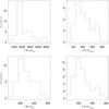 |
Fig. 2 Histograms of the FWHM of the emission lines in km s-1. From left to right and top to bottom: FWHM of BC, [SII], NC and [NII]. All FWHM were corrected by the instrumental width. |
4. Nuclear dynamics
4.1. Virial BH masses
Black holes are very important in the study of active galaxies. They constitute a fundamental parameter to understand the mechanisms involved in the nuclear regions of AGNs and could also provide information about the process of galaxy formation. If we assume that the BLR clouds are isotropically spatially and kinematically distributed, MBH is related to the radius of the BLR (RBLR) and the mean cloud velocity v inside it as MBH = RBLRv2G-1. According to Greene & Ho (2005), BH masses can be calculated through luminosity and FWHM of the same Balmer line, as follows: 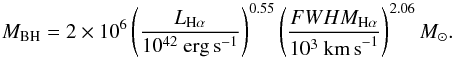 (1)This method is highly useful because Balmer lines are easily detectable even in distant AGNs. However, this equation can be applied only to AGNs that show broad component lines, thereby the importance of performing Gaussian deconvolution to Balmer lines such as described in Sect. 3. Using Eq. (1) we determined MBH of our sample by taking into account the BC of Hα after correcting for instrumental resolution. Table A.2 specifies the galaxy name, FWHM, and luminosity of BC and BH masses. Figure 3 shows the distribution of BH masses, whose typical uncertainties are around ~0.1 dex. Almost all of the BH masses are between log (MBH/M⊙) ~ 5.75 and 7.35 (mean value ~6.2). Only two objects show masses log (MBH/M⊙) ≥ 7.5; these objects are 6dF J1117042−290233, RX J2301.8−5508, which have log (MBH/M⊙) of 7.7 and 7.5, respectively. There are also a few determinations of low-mass BHs with log (MBH/M⊙) < 5.5, mainly due to their low BC luminosities. These galaxies are SDSS J144052.60−023506.2, Zw374.029 with log (MBH/M⊙) = 5.4 and NPM1G−17.0312 with log (MBH/M⊙) = 5.3.
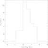 |
Fig. 3 Histogram of the black hole masses of the sample. |
4.2. The MBH − σ⋆ relation
Possible correlations between BH masses and properties of the host galaxies are of fundamental importance to understand the galaxy formation processes and evolution. The relations between black hole masses and the velocity dispersion of the bulge have been studied by several authors, such as Ferrarese & Merritt (2000) and Gebhardt et al. (2000). Tremaine et al. (2002), in the attempt to relate some galaxy properties to central BHs, found that BH masses for normal galaxies could be estimated with the relation,  (2)On the other hand, in a sample of 14 Seyfert 1 galaxies, Nelson et al. (2004) measured the bulge stellar velocity dispersion and determined their SMBH masses using the reverberation mapping technique and found that the Seyfert galaxies followed the same MBH − σ⋆ relation as nonactive galaxies.
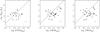 |
Fig. 4 MBH − σ⋆ relation for the galaxies of the sample, using the FWHM of [SII] (left), [NII] (middle), and the narrow component NC of Hα (right). All FWHM are in km s-1 and were corrected by the instrumental width. The solid line represents the relation given by Tremaine et al. using FWHM = 2.35σ⋆. Typical error bars are on each plot. |
Usually it is difficult to determine the stellar velocity dispersions in AGNs because of the strong nonstellar continuum that dilutes the absorption lines of the underlying stellar populations. On the other hand, gas emission lines are an important feature in AGNs and they are detectable even in distant galaxies, unlike stellar absorption lines. Because of this, some authors (e.g., Nelson 2000; Komossa & Xu 2007) use, for instance, [OIII] or [SII] lines instead the stellar velocity dispersion to study the MBH − σ⋆ relation. For example, when the width of the narrow [OIII]λ5007 emission line is used, most authors found that in general NLS1 galaxies do not follow the MBH − σ⋆ relation (Grupe & Mathur 2004; Bian et al. 2006; Watson et al. 2007). Nevertheless, Wang & Lu (2001), Wandel (2002) found that NLS1 follow the relation but with a larger scatter than for normal galaxies.
In Fig. 4 we plot BH masses against FWHMgas, where the solid line represents MBH − σ⋆ relation for normal galaxies (Tremaine et al. 2002). We explore the MBH − σ⋆ relation using FWHMgas instead of σ⋆, where FWHMgas refers to the FWHM of the emission lines NC of Hα, [NII], and [SII]. We take these widths as possible proxys of σ⋆, by taking into account the relation FWHM = 2.3548 × σ for a Gaussian profile of these lines.
Taking the uncertainties of our determinations on FWHMgas and black hole masses into account, Fig. 4 shows that, in general, most of the objects lie systematically below the MBH − σ⋆ relation for normal nuclei. In the case of [NII], around 70% of the galaxies lie below the Tremaine line. The higher deviation is seen using the NC of Hα, where ~80% of the objects lie below the MBH − σ⋆ relation. In the case of [SII] lines, NLS1s are closer to the relation and ~45% of the targets lie above the relation. This agrees with previous results of Komossa & Xu (2007). Despite the objects being closer to the Tremaine relation, they are slightly below it and we do not find any evidence of correlation among the FWHM of [SII] lines and the BH mass. The cases studied here of [SII], [NII], and NC lines are in agreement with the idea of that NLS1 may mainly reside in galaxies with pseudobulges (Mathur et al. 2012). In this scenario, NLS1 do not follow the MBH − σ⋆ because their bulges are intrinsically different from those of other galaxies.
Otherwise, the fact that, in general, NLS1 lie systematically below the MBH − σ⋆ relation for the three studied cases, could imply that NLS1 galaxies have lower BH masses compared to those that follow the relation. It is well known that NLS1 have high Eddington ratios (Warner et al. 2004) and related to that, Mathur (2000) proposed that NLS1 are analogous objects to high-redshift quasars (z> 4). This way, NLS1 may be in an early evolutionary phase that occupies young host galaxies. It is not very clear how the displacement of NLS1 would be along the MBH − σ⋆ relation, but the fact that NLS1 have high Eddington ratios suggest that their black hole masses must be rapidly growing (Mathur & Grupe 2005a,b). In this scenario, the NLS1 tracks on the MBH − σ⋆ would be upward.
4.3. The intermediate component of Hα
In Sect. 3 we mentioned that, besides the narrow and broad components for Hα, for some objects it was necessary to include an additional kinematical intermediate component to fit the line. The sum of only two components (BC and NC) did not fit the profile of Hα well for some galaxies of our sample, thus giving residuals that were considerably higher than the spectral noise and requiring an additional component. Indeed, several components for the Balmer emission lines were detected in some AGNs (Popović et al. 2004; Zhu et al. 2009b) and NLS1s (Zhu et al. 2009a; Mullaney & Ward 2008). While by definition BC and NC have a direct association with the BLR and NLR, respectively, described in the standard scenario for Seyferts, the IC remains clearly related to a well-known physical region. Various authors, for example, Zhu et al. (2009a) and Zhu et al. (2009b), claimed that the emission from the BLR can be described by two Gaussian profiles, one very broad and an intermediate component. Both of these emissions could be originated in two different regions, each one with different velocity dispersions and spatially associated, but there is no clear scheme yet. To explore this kinematical component, we used our data from the IC detected in our sample.
Following the procedure described in Sect. 3 we determined the IC for 14 galaxies (37% of the sample). The main results involving FWHM of Hα IC are presented in Fig. 5. The distribution of the FWHM (top left panel of Fig. 5) of IC shows that for 11 out of 14 galaxies, the FWHM of IC is in the range of 600−1500 km s-1 with mean value of ~1100 km s-1. We note that the shape of the distributions for IC, BC, and NC are apparently similar. So, we have applied a Kolmogorov-Smirnov (K-S) test and confirmed that the distribution of the IC is significantly different from those of NC and BC with P< 10-8 and P< 10-5, respectively, as being drawn from the same parent distribution. This suggests the possibility of three kinematically distinct emitting regions: the well-known BLR and NLR, and an intermediate line region (ILR).
Comparing the FWHMIC and FWHMBC we found that they are strongly related (top right panel). An OLS bisector fit gives a slope of ~2.4 with a small (<100 km s-1) zero point and a remarkable Pearson correlation coefficient of rp = 0.93. We calculated the ratio between the two quantities (bottom left panel), and we find a mean value of FWHMBC/FWHMIC ~ 2.5, which is somewhat lower than that obtained by Mao et al. (2010) of ~3 for Hβ.
We have to keep in mind that the BH masses determinations (Eq. (1)) involves the BC, so we would expect a relation between the FWHMIC and the BH mass, which is actually seen in the bottom right panel of Fig. 5. An OLS bisector fit gives a slope of ~4.4 and a zero point of log (MBH/M⊙) ~ −6.5. A Pearson correlation coefficient of rp = 0.86 shows the close relation between them, suggesting that the dynamics of the ILR is somehow affected by the central BH. We tested whether some of these relations depend on another parameter, such as the luminosity of the lines, but we did not find any dependence on them. A particular case is presented by the galaxy HE1107+0129, which presents an additional component of ~290 km s-1 (see Sect. 6), and was not taken into account for the analysis in Fig. 5 and in the bottom right plot in Fig. 6. Besides this galaxy, IGRJ16185−5928 was not taken into account in the bottom right plot of Fig. 5 because of its high deviation from the remaining points.
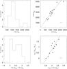 |
Fig. 5 Histogram of the FWHM of intermediate component (IC) of Hα (top left), the relation between the FWHM of BC and the FWHM of IC (top right), the histogram of FWHMBC/FWHMIC (bottom left), and the relation between BH masses and the FWHM of IC (bottom right). All FWHM are in units of km s-1. Typical error bars are shown. Solid lines represent the best fits for our data. |
The tight relationship between FWHMBC and FWHMIC makes us wonder if there is another quantity governing this behavior. We do not have any information about the possible location of the origin of the IC. So far, we only know that, in the frame of the standard scenario for AGNs, BC and NC originate in the BLR and NLR regions, respectively; these two regions are very different in size, extension, geometry, kinematics, and physical conditions. The IC detected in our sample tells us that there could be another physical region. Under the assumption that the square of the FWHM of the gas decreases with the distance to the center, this ILR is possibly surrounding the BLR and could be located outside, although near the BLR with a ratio of mean sizes in a proportion given by the square of the ratio between the two FWHMs. This way the ratio of both would be RILR/RBLR ∝ (FWHMBLR/FWHMILR)2 ~ 4−9.
5. Luminosities
We determined the luminosity for each component of Hα, as well as for [NII] and [SII] lines. Figure 6 shows the luminosities of BC compared to those of NC (top left panel), [NII]λ6584 (top right), [SII]λ6731 (bottom left), and IC (bottom right).
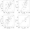 |
Fig. 6 Luminosity of BC compared with those of the NLR: NC (top left), [SII] (top right), [NII] (bottom left), and with the IC (bottom right). All luminosities are in units of erg s-1. Solid lines represent the best fits for our data. Typical error bars are shown in each plot. |
The luminosities of BC are systematically higher than those of the lines originated at the NLR ([NII], [SII], and NC), and that of the IC, and a relation is evident between them. We found that the luminosity of the BC is typically eight times the luminosity of the NC, and only two objects (2MASXJ21565663−1139314 and SDSSJ144052.60−023506.2) present similar or lower luminosity of the BC compared to that of the NC. A similar trend is observed when comparing BC to [NII]λ6584 and [SII]λ6731. In the case of the IC, the luminosities of the BC are slightly higher for 10 out of 13 objects, and the remaining present weak BCs, and thus they have very low luminosities.
We applied OLS bisector fits to these data, which give slopes of around 1.2, 1.2, and 1.3 for NC, [NII], and [SII] lines, respectively. The Pearson coefficients are typically around rp = 0.67 for these three relations. The slopes of the relations between the BC luminosity and that of the lines arising in the NLR are similar, which could suggest that the ionizing source is the same in the three cases. Interestingly, there is a stronger relationship between the BC and IC luminosities: the OLS bisector fit gives a slope of ~0.84 and a Pearson correlation coefficient of 0.90, which probably implies a dependence among their emitting regions and also possibly on their physical conditions. The fact that for this case the slope is slower than that for narrow lines could suggest a possible physical difference between the emitting regions (ILR and NLR). Curiously, comparing LBC to LIC, they are quite similar with a mean value of LBC/LIC ~ 1.5. This interesting result tells us that the luminosities of both regions are indeed comparable. The geometry of the emitting regions and the presence of different amount of gas in each region probably play an important role on their luminosities. Nonetheless, this is not the case for the ILR, for which, even though physical conditions are not well known yet, the relation between BC and IC is stronger than for NLR lines.
6. Some curious cases
Two objects show higher velocity dispersion for the IC. These galaxies are 6dF J1117042−290233 and IGRJ16185−5928, which have FWHM of ~1700 and ~2000 km s-1, respectively. They also show the higher velocity dispersion for the BC, ~5000 km s-1, and the highest black hole masses, log (MBH/M⊙) > 7.3.
We do not detect any BC for Zw037.022, which only has a NC for this Balmer line of ~130 km s-1. According to Moran et al. (1996) and Kollatschny et al. (2008), this object has been classified as Sy1 and NLS1, respectively. On the other hand, according to the spectral classification of the Sloan Digital Sky Survey Data Release 12 (SDSS DR12; Alam et al. 2015; Eisenstein et al. 2011), Zw037.022 is a star forming galaxy. This classification is based on whether the galaxy has detectable emission lines that are consistent with star formation according to the criteria log ([OIII]λ500/Hα) < 0.7−1.2(log ([NII]λ6584/Hα) + 0.4). In our case, we find that log ([NII]λ6584/Hα) = −0.8, log ([SII]λ6716/Hα) = −0.8, and log ([SII]λ6731/Hα) = −0.9. These results agree with the idea of that this object must be classified as a star forming galaxy. In addition, the fact that this galaxy does not show a BC supports the idea that it is neither a Sy1 nor a NLS1 galaxy.
As stated in Sect. 4.3, the object HE1107+0129 shows an additional component of ~290 km s-1. We tried to fit the spectrum of this galaxy with only two components for Hα, but the residuals were much higher than the noise of the spectrum, and so another component was necessary. This extra component is comparable with the FWHM distribution of NC and shows a blueshift of ~360 km s-1 compared to the NC (FWHM of ~190 km s-1). We analyzed the relation between the FWHM of BC and NC for the sample and the medium value is FWHMBC/FWHMNC ~ 8. For this galaxy, the ratio between the FWHMBC and the FWHM of this additional component is also ~8. These facts suggest that this extra component is emitted from the NLR and not from an ILR. For this reason, it was not taken into account in the analysis of Sect. 4.3.
7. Final remarks
We have observed and analyzed the spectroscopic data of a sample of 36 NLS1 galaxies, 27 of which are in the Southern Hemisphere. We performed careful Gaussian decomposition to the main emission lines in the red spectral range. Several components were fitted to the global profile for Hα +[NII]λλ6548,6583. This allowed us to estimate the virial BH masses of the galaxies. The obtained values for our sample are in the range log (MBH/M⊙) = 5.3−7.7, where the mean value is around log (MBH/M⊙) = 6.2. The black hole masses are in the range log (MBH/M⊙) = 5.7−7.3 for 32 out of 36 galaxies. These values are lower that those found in broad line Seyfert 1 galaxies, confirming that on average, NLS1 have lower BH masses (e.g., Komossa & Xu 2007; Grupe 2004).
We tested the narrow component of Hα, [NII], and [SII] lines as proxys of σ⋆, using the FWHM of these emission lines to examine the MBH − σ⋆ relation for normal galaxies. Taking into account the uncertainties of our determinations on the FWHM of the emission lines and black hole masses, we found that in general most of our NLS1s lie below the MBH − σ⋆ relation for normal galaxies. The fact that NLS1 have lower black hole masses, and taking into account that they have high acretion rates (Warner et al. 2004) and therefore their black hole mass are growing quickly (Mathur & Grupe 2005a,b), could suggest that such AGNs are at an early stage of nuclear activity. Although in the case of the [SII] lines the galaxies seem to be closer to the relation than the other lines (in agreement with Komossa & Xu 2007, results), we do not see any correlation between the FWHM of [SII] lines and the BH mass. The fact that the three tested emission lines put the NLS1 below the MBH − σ⋆ relation could be in agreement with Mathur et al. (2012), who found that such AGNs are mainly hosted by galaxies with pseudobulges. Related to this, NLS1 would not follow the MBH − σ⋆ because their bulges are different from those of other AGN types.
We studied the intermediate component of Hα found in 13 out of 36 galaxies. Comparing the distribution of velocities between the three components of Hα, we see that the FWHM of BC is between 900−3200 km s-1 with a peak in 1600 km s-1 for most objects; the IC is in the velocity range 700−1500 km s-1 for most galaxies, with most objects showing FWHM of 1100 km s-1; while for the NC the velocity range is 180−500 km s-1 with a peak in 220 km s-1. We note a high correlation between FWHMIC and FWHMBC, with a Pearson correlation coefficient of rp = 0.93. We found for our sample that FWHMBC/FWHMIC is in a range of 2.1−3 with a mean value of ~2.5, which is somewhat lower than that obtained by Mao et al. (2010) of ~3 for Hβ. We also performed Kolmogorov-Smirnov (K-S) tests to FWHMBC and FWHMIC, and to FWHMNC and FWHMIC, which give probabilities of P< 10-5 and P< 10-8 as being drawn from the same parent distribution, respectively. All these results point out the possibility of three kinematically distinct emitting regions and show that BC and IC are somehow linked, possibly implying that IC could arise in a region surrounding the BLR. Taking into account that BH masses depend on FWHMBC, and FWHMIC correlates with FWHMBC, it is expected to find a correlation between BH masses and FWHMIC. In fact, this correlation has a Pearson correlation coefficient rp = 0.86, suggesting that the dynamics of this emitting region is clearly affected by the central engine.
The presence of the additional intermediate component mainly affects the NC. If only two components were used to fit the Hα line, NC would be much broader and would show a greater amount of line flux. In the case of the BC, it does not vary significantly; in general it could increase its FWHM by ~10% and decrease the flux by ~10−25%. Contrary to what we expected, BH masses in general decrease ~10−20% if one consider only two components for this Balmer line.
We also studied the emission line luminosities of broad and narrow lines. There are some tendencies between the BC luminosity and those of the narrow lines [NII], [SII], and NC with Pearson correlation coefficients around 0.67 for the three cases, indicating that the emission in BLR and NLR are proportional. Interestingly, their slopes are similar, around 1.2, as derived from OLS bisector fits. The relation is even stronger for the IC with a slope of around 0.84 and a Pearson correlation coefficient of 0.90. The fact that the slope is different for the NC and the IC lines would indicate possible physical difference between the regions. Interestingly, we found that the luminosities of BC and IC are comparable with a mean value LBC/LIC ~ 1.5. Related to this, the geometry of the emitting regions, despite distinct amounts of gas present in each one, play an important role. Even
though the physical conditions of the ILR are not well known yet, our results suggest that this region is different from the BLR and NLR, with properties that are somehow related and strongly linked to those of the BLR.
IRAF: the Image Reduction and Analysis Facility is distributed by the National Optical Astronomy Observatories, which is operated by the Association of Universities for Research in Astronomy, Inc. (AURA) under cooperative agreement with the National Science Foundation (NSF).
Acknowledgments
This work was partially supported by Consejo de Investigaciones Científicas y Técnicas (CONICET) and Secretaría de Ciencia y Técnica de la Universidad Nacional de Córdoba (SecyT). We want to thank the anonymous referee, whose very useful remarks helped us to improve this paper. This research has made use of the NASA/IPAC Extragalactic Database (NED) which is operated by the Jet Propulsion Laboratory, California Institute of Technology, under contract with the National Aeronautics and Space Administration.
References
- Alam, S., Albareti, F. D., Allen de Prieto, C., et al. 2015, ApJS, 219, 12 [NASA ADS] [CrossRef] [Google Scholar]
- Bian, W., & Zhao, Y. 2004, MNRAS, 347, 607 [NASA ADS] [CrossRef] [Google Scholar]
- Bian, W., Yuan, Q., & Zhao, Y. 2006, MNRAS, 367, 860 [NASA ADS] [CrossRef] [Google Scholar]
- Botte, V., Ciroi, S., di Mille, F., Rafanelli, P., & Romano, A. 2005, MNRAS, 356, 789 [NASA ADS] [CrossRef] [Google Scholar]
- Brotherton, M. S., Wills, B. J., Francis, P. J., & Steidel, C. C. 1994, ApJ, 430, 495 [NASA ADS] [CrossRef] [Google Scholar]
- Corbin, M. R., & Francis, P. J. 1994, AJ, 108, 2016 [NASA ADS] [CrossRef] [Google Scholar]
- Crenshaw, D. M., & Kraemer, S. B. 2007, ApJ, 659, 250 [NASA ADS] [CrossRef] [Google Scholar]
- Crenshaw, D. M., Kraemer, S. B., Schmitt, H. R., et al. 2009, ApJ, 698, 281 [NASA ADS] [CrossRef] [Google Scholar]
- Eisenstein, D. J., Weinberg, D. H., Agol, E., et al. 2011, AJ, 142, 72 [Google Scholar]
- Ferrarese, L., & Merritt, D. 2000, ApJ, 539, L9 [NASA ADS] [CrossRef] [Google Scholar]
- Gebhardt, K., Bender, R., Bower, G., et al. 2000, ApJ, 539, L13 [NASA ADS] [CrossRef] [Google Scholar]
- Goodrich, R. W. 1989, ApJ, 342, 224 [NASA ADS] [CrossRef] [Google Scholar]
- Greene, J. E., & Ho, L. C. 2005, ApJ, 630, 122 [NASA ADS] [CrossRef] [Google Scholar]
- Grupe, D. 2004, AJ, 127, 1799 [NASA ADS] [CrossRef] [Google Scholar]
- Grupe, D., & Mathur, S. 2004, ApJ, 606, L41 [NASA ADS] [CrossRef] [Google Scholar]
- Hu, C., Wang, J.-M., Ho, L. C., et al. 2008, ApJ, 683, L115 [NASA ADS] [CrossRef] [Google Scholar]
- Kollatschny, W., Kotulla, R., Pietsch, W., Bischoff, K., & Zetzl, M. 2008, A&A, 484, 897 [NASA ADS] [CrossRef] [EDP Sciences] [Google Scholar]
- Komossa, S., & Xu, D. 2007, ApJ, 667, L33 [NASA ADS] [CrossRef] [Google Scholar]
- Mao, W., Hu, C., Wang, J., et al. 2010, Science China Physics, Mechanics, and Astronomy, 53, 2307 [NASA ADS] [CrossRef] [Google Scholar]
- Mason, K. O., Puchnarewicz, E. M., & Jones, L. R. 1996, MNRAS, 283, L26 [NASA ADS] [CrossRef] [Google Scholar]
- Mathur, S. 2000, MNRAS, 314, L17 [NASA ADS] [CrossRef] [Google Scholar]
- Mathur, S., & Grupe, D. 2005a, A&A, 432, 463 [NASA ADS] [CrossRef] [EDP Sciences] [Google Scholar]
- Mathur, S., & Grupe, D. 2005b, ApJ, 633, 688 [NASA ADS] [CrossRef] [Google Scholar]
- Mathur, S., Kuraszkiewicz, J., & Czerny, B. 2001, New Astron., 6, 321 [NASA ADS] [CrossRef] [Google Scholar]
- Mathur, S., Fields, D., Peterson, B., & Grupe, D. 2012, ApJ, 754, 146 [NASA ADS] [CrossRef] [Google Scholar]
- Moran, E. C., Halpern, J. P., & Helfand, D. J. 1996, ApJS, 106, 341 [NASA ADS] [CrossRef] [Google Scholar]
- Mullaney, J. R., & Ward, M. J. 2008, MNRAS, 385, 53 [NASA ADS] [CrossRef] [Google Scholar]
- Nelson, C. H. 2000, ApJ, 544, L91 [NASA ADS] [CrossRef] [Google Scholar]
- Nelson, C. H., Green, R. F., Bower, G., Gebhardt, K., & Weistrop, D. 2004, ApJ, 615, 652 [NASA ADS] [CrossRef] [Google Scholar]
- Osterbrock, D. E., & Pogge, R. W. 1985, ApJ, 297, 166 [NASA ADS] [CrossRef] [Google Scholar]
- Pogge, R. W., & Owen, J. M. 1993, OSU Internal Report, 93-01 [Google Scholar]
- Popović, L. Č., Mediavilla, E., Bon, E., & Ilić, D. 2004, A&A, 423, 909 [NASA ADS] [CrossRef] [EDP Sciences] [Google Scholar]
- Tremaine, S., Gebhardt, K., Bender, R., et al. 2002, ApJ, 574, 740 [NASA ADS] [CrossRef] [Google Scholar]
- Véron-Cetty, M.-P., & Véron, P. 2010, A&A, 518, A10 [NASA ADS] [CrossRef] [EDP Sciences] [Google Scholar]
- Wandel, A. 2002, ApJ, 565, 762 [NASA ADS] [CrossRef] [Google Scholar]
- Wang, T., & Lu, Y. 2001, A&A, 377, 52 [NASA ADS] [CrossRef] [EDP Sciences] [Google Scholar]
- Warner, C., Hamann, F., & Dietrich, M. 2004, ApJ, 608, 136 [NASA ADS] [CrossRef] [Google Scholar]
- Watson, L. C., Mathur, S., & Grupe, D. 2007, AJ, 133, 2435 [NASA ADS] [CrossRef] [Google Scholar]
- Williams, R. J., Pogge, R. W., & Mathur, S. 2002, AJ, 124, 3042 [NASA ADS] [CrossRef] [Google Scholar]
- Zhou, H., Wang, T., Yuan, W., et al. 2006, ApJS, 166, 128 [NASA ADS] [CrossRef] [Google Scholar]
- Zhu, L., Zhang, S., & Tang, S. 2009a, ArXiv e-prints [arXiv:0901.2167] [Google Scholar]
- Zhu, L., Zhang, S. N., & Tang, S. 2009b, ApJ, 700, 1173 [NASA ADS] [CrossRef] [Google Scholar]
Appendix A: Additional data
Observed galaxies.
FWHM of the BC of Hα, luminosity of that component, and BH masses.
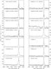 |
Fig. A.1 Observed spectra of the NLS1 in the range 5800−6800 Å at rest frame. |
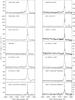 |
Fig. A.1 continued. |
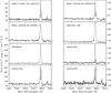 |
Fig. A.1 continued. |
All Tables
All Figures
|
Fig. 1 From left to right: Gaussian decomposition for the galaxies MCG04.24.017, 2MASXJ05014863−2253232, and 2MASX J21124490− 3730119, respectively. Thick line represents the spectra; the Hα components and [NII]λ6548,6584 are shown in dotted lines. The residuals are plotted at the bottom of each panel and were displaced from zero for clarity. |
| In the text | |
|
Fig. 2 Histograms of the FWHM of the emission lines in km s-1. From left to right and top to bottom: FWHM of BC, [SII], NC and [NII]. All FWHM were corrected by the instrumental width. |
| In the text | |
|
Fig. 3 Histogram of the black hole masses of the sample. |
| In the text | |
|
Fig. 4 MBH − σ⋆ relation for the galaxies of the sample, using the FWHM of [SII] (left), [NII] (middle), and the narrow component NC of Hα (right). All FWHM are in km s-1 and were corrected by the instrumental width. The solid line represents the relation given by Tremaine et al. using FWHM = 2.35σ⋆. Typical error bars are on each plot. |
| In the text | |
|
Fig. 5 Histogram of the FWHM of intermediate component (IC) of Hα (top left), the relation between the FWHM of BC and the FWHM of IC (top right), the histogram of FWHMBC/FWHMIC (bottom left), and the relation between BH masses and the FWHM of IC (bottom right). All FWHM are in units of km s-1. Typical error bars are shown. Solid lines represent the best fits for our data. |
| In the text | |
|
Fig. 6 Luminosity of BC compared with those of the NLR: NC (top left), [SII] (top right), [NII] (bottom left), and with the IC (bottom right). All luminosities are in units of erg s-1. Solid lines represent the best fits for our data. Typical error bars are shown in each plot. |
| In the text | |
|
Fig. A.1 Observed spectra of the NLS1 in the range 5800−6800 Å at rest frame. |
| In the text | |
|
Fig. A.1 continued. |
| In the text | |
|
Fig. A.1 continued. |
| In the text | |
Current usage metrics show cumulative count of Article Views (full-text article views including HTML views, PDF and ePub downloads, according to the available data) and Abstracts Views on Vision4Press platform.
Data correspond to usage on the plateform after 2015. The current usage metrics is available 48-96 hours after online publication and is updated daily on week days.
Initial download of the metrics may take a while.