| Issue |
A&A
Volume 596, December 2016
|
|
|---|---|---|
| Article Number | A36 | |
| Number of page(s) | 20 | |
| Section | The Sun | |
| DOI | https://doi.org/10.1051/0004-6361/201629109 | |
| Published online | 25 November 2016 | |
A model for straight and helical solar jets
II. Parametric study of the plasma beta
1 LESIA, Observatoire de Paris, PSL Research University, CNRS, Sorbonne Universités, UPMC Univ. Paris 06, Univ. Paris Diderot, Sorbonne Paris Cité, 5 place Jules Janssen, 92195 Meudon, France
e-mail: This email address is being protected from spambots. You need JavaScript enabled to view it.
2 CISL/HAO, National Center for Atmospheric Research, PO Box 3000, Boulder, CO 80307-3000, USA
3 Heliophysics Science Division, NASA Goddard Space Flight Center, Greenbelt, MD 20771, USA
Received: 14 June 2016
Accepted: 27 September 2016
Abstract
Context. Jets are dynamic, impulsive, well-collimated plasma events that develop at many different scales and in different layers of the solar atmosphere.
Aims. Jets are believed to be induced by magnetic reconnection, a process central to many astrophysical phenomena. Within the solar atmosphere, jet-like events develop in many different environments, e.g., in the vicinity of active regions, as well as in coronal holes, and at various scales, from small photospheric spicules to large coronal jets. In all these events, signatures of helical structure and/or twisting/rotating motions are regularly observed. We aim to establish that a single model can generally reproduce the observed properties of these jet-like events.
Methods. Using our state-of-the-art numerical solver ARMS, we present a parametric study of a numerical tridimensional magnetohydrodynamic (MHD) model of solar jet-like events. Within the MHD paradigm, we study the impact of varying the atmospheric plasma β on the generation and properties of solar-like jets.
Results. The parametric study validates our model of jets for plasma β ranging from 10-3 to 1, typical of the different layers and magnetic environments of the solar atmosphere. Our model of jets can robustly explain the generation of helical solar jet-like events at various β ≤ 1. We introduces the new result that the plasma β modifies the morphology of the helical jet, explaining the different observed shapes of jets at different scales and in different layers of the solar atmosphere.
Conclusions. Our results enable us to understand the energisation, triggering, and driving processes of jet-like events. Our model enables us to make predictions of the impulsiveness and energetics of jets as determined by the surrounding environment, as well as the morphological properties of the resulting jets.
Key words: magnetohydrodynamics (MHD) / Sun: flares / magnetic reconnection / Sun: magnetic fields
© ESO, 2016
1. Introduction
In the solar atmosphere, jet-like structures, defined by an impulsive evolution of a thin collimated bright or dark structure that extends along a particular direction, are ubiquitous. Jet-like events are observed in a wide range of environments, on scales ranging from the limit of instrumental resolution to hundreds of Mm. They have been detected in almost all wavelengths available to observers, and have thus acquired a multitude of names: spicules (e.g., Sterling 2000; De Pontieu et al. 2007); photospheric jets (e.g., Nishizuka et al. 2008, 2011); chromospheric Hα surges (e.g., Schmieder et al. 1995); chromospheric Ca II H jets (e.g., Morita et al. 2010); coronal EUV jets and macrospicules (e.g., Nisticò et al. 2009; Kamio et al. 2010); coronal X-ray jets (e.g., Savcheva et al. 2007); and white-light polar jets (e.g., Wang & Sheeley 2002). Multi-wavelength observations show slightly different spatial, physical, and temporal properties in each observational bandwidth, revealing that each jet event is formed of multi-thermal and multi-velocity plasmas (e.g., Chifor et al. 2008a; Madjarska 2011; Tian et al. 2014).
In addition to the basic morphological properties that allows all these events to qualify as jets, several other features and properties have been observed in some particular events independently of the scale. Recent high-resolution observations have shown that the base of some chromospheric jets (Liu et al. 2011b; Zeng et al. 2016) have the same morphology and presence of bi-directional flows seen in examples of larger-scale coronal jets (Shibata et al. 1992). This suggests that they may share a common underlying topological structure: a 3D null point and its fan/spine separatrices (Moreno-Insertis et al. 2008; Liu et al. 2011a; Zhang et al. 2012; Zeng et al. 2016). Regarding the morphology of the spire, using Hinode data, Suematsu et al. (2008) and latter Sterling et al. (2010b) have noted that spicules present a double-stranded morphology that is similar to the emission pattern observed in coronal jets. Supersonic, though possibly sub-Alfvénic velocities have also been noted for chromospheric events (Tian et al. 2014), as well as jets developing in the corona (Cirtain et al. 2007). Jet-like events also tend to recur homologously at the same location independently of their size; this property has been commonly observed for spicules (De Pontieu et al. 2007), chromospheric jets (Tian et al. 2014), and coronal jets (Jiang et al. 2007; Chifor et al. 2008b,a).
One of the most puzzling properties that all these events display is the common presence of helical structure and/or twisting motion. Signatures of a rotating structure are present in a noticeable sample of all these phenomena in spite of their very different environments. On the greater end of the spatial scale, the existence of helical properties has been very frequently noticed with a broad range of techniques. First, the morphology of the coronal jets has been noted from X-ray and EUV images by various studies (e.g., Shibata et al. 1992; Canfield et al. 1996; Jiang et al. 2007; Shen et al. 2012). The frequency of a helical structure in coronal jets is strongly dependent on the wavelength of observation. By looking only at X-ray images, Shimojo et al. (1996) reported a 10% occurrence of twisting within their observational sample. Using more recent Hinode/XRT observations, Savcheva et al. (2009) noted that 14% of their X-ray jets showed signs of twisting. In contrast, using EUV observations from the STEREO mission (Kaiser et al. 2008), Nisticò et al. (2009) found that 31 out of 79 jet events presented a clear helical structure. From a sample of 54 jets observed in X-rays, Moore et al. (2013) found that 29 out of the 32 jets that also presented a cool component of emission at SDO/AIA 304 Å displayed a rotation about its axis in that channel. Helical structure and twisting motion are thus predominantly noted in the cooler EUV lines, such as 304 Å. Using that particular bandwidth, several studies (e.g., Shen et al. 2011; Chen et al. 2012; Hong et al. 2013) have inferred the twisting rate and the helical morphology by analysing the motion of well identified features within the jet structure.
The helical shape and twisting have been further demonstrated by more advanced methods. Exploiting the stereoscopic capabilities of the joint observations by the two STEREO spacecrafts, Patsourakos et al. (2008) reconstructed a coronal jet in 3D and unambiguously revealed its helical shape. Doppler images have also been used to show that several coronal jet events presented strong rotational motions, blue- and red-shifts being observed on opposite sides of each jet (Dere et al. 1989; Pike & Mason 1998; Harrison et al. 2001; Jibben & Canfield 2004; Cheung et al. 2015). Combined spectroscopic and stereoscopic observations of a jet have been carried out by Kamio et al. (2010), who also recovered its helical structure and confirmed its rotating nature during the event.
Following the conceptual ideas of Shibata & Uchida (1985), Shibata & Uchida (1986), Canfield et al. (1996), and Jibben & Canfield (2004), in recent years several numerical works have suggested and shown evidence that helical jets were driven/accelerated at least partly due to propagating nonlinear Alfvénic waves (Török et al. 2009; Pariat et al. 2009, 2010, 2015a; Lee et al. 2015). As discussed in Sect. 2 of Pariat et al. (2015a, hereafter PDD15), three main physical processes might explain the acceleration of the plasma: the tension-driven upflows that directly result from the local dynamics of the reconnected field line at the reconnection site; the evaporation upflows that are induced by the heat/pressure gradients in the reconnected field lines (heat created directly by the reconnection process or secondarily after accelerated particles have interacted with the plasma); and the untwisting upflows that are induced by a global reconfiguration of the helicity within the newly opened magnetic field lines. Magnetic reconnection between closed twisted field lines and open untwisted lines (or large-scale closed surrounding field lines, as in Wyper & DeVore 2016) reconfigures the system and generates the untwisting upflows: a nonlinear kink wave develops upward along each reconnected field line in order to distribute the twist along the whole extent of the field line. The compressive component of the nonlinear wave induces compression and heating of the plasma and creates an upward bulk flow of material. The overall helical jet is the result of the sequential reconnection of multiple field lines.
Török et al. (2009), in a zero-β simulation, showed the upward propagation of a pure torsional/kink wave that they associated with the jet (see their Fig. 4). Pariat et al. (2009, 2010, 2015a), in β = 0.25 cases, also argued that the helical jet consisted of untwisting upflows driven by the propagation of torsional waves: these waves were induced by the sequential reconnection of twisted closed field lines with the straight open field. Figure 4 of (Pariat et al. 2009, hereafter PAD09), as well as Fig. 1 of PDD15, showed the dynamics of the magnetic field lines with the upward propagation of the twist along individual field lines. PAD09 further showed that the velocity of this propagating wave was Alfvénic (0.65cA–0.90cA), while the actual bulk plasma speed was much smaller (cf. their Fig. 6). Figures 10 and 11 of PAD09 showed the magnetic helicity flux, the Poynting flux and the fluxes of kinetic and magnetic energy at different heights, further confirming the upward propagation of energy and helicity at near-Alfvén speed due to the global Alfvénic nonlinear wave trains. In other numerical models of coronal jets generated in response to flux emergence, Archontis & Hood (2013) also hypothesised that helical jets were driven by untwisting upflows. Based on the same model, Lee et al. (2015) found further evidence that the untwisting motion is associated with a propagating torsional wave. Fang et al. (2014) also observed untwisting upflows driving high-density plasma upward due to the Lorentz force associated with the magnetic tension in the non-linear Alfven waves dominating the divergence of the Poynting flux. They showed that thermal conduction was a second-order effect, only marginally enhancing the upflow of material by 2%.
At smaller scales, evidence of rotating motions has also been deduced for chromospheric/transition region jet events. Liu et al. (2009, 2011b) carried out a thorough analysis of a jet observed in Ca II in the vicinity of an active region, and found multiple signs of the untwisting dynamics of the chromospheric jet. Tian et al. (2014) studied a sample of chromospheric events with the IRIS instrument (De Pontieu et al. 2014b), and noted obvious transverse motions as well as line broadenings that they attributed to the existence of twist and torsional Alfvén waves. At the photospheric level, there is accumulating evidence that an important fraction of spicules present twisting motions (Sterling et al. 2010a,b; De Pontieu et al. 2012). The recent IRIS data indicate that twisting/torsional motions are extremely frequent within the chromosphere and are associated with spicules De Pontieu et al. (2014a). At even smaller scale, beyond the resolution of imaging instruments, the spectrum of explosive events can also be interpreted as arising from the fast rotation of magnetic structures (Curdt & Tian 2011; Curdt et al. 2012).
Although all these events develop in environments that exhibit substantial differences in temperature, pressure, plasma density, and even level of ionisation, some common characteristics are certainly shared between the jet-like structures. The idea that some common mechanism is triggering and/or driving some of these different classes of events has thus naturally developed (Shibata et al. 2007; Moore et al. 2013; Cranmer & Woolsey 2015). We build on that idea by aiming to assess how well a model originally developed for large-scale coronal jets PAD09 can explain the properties of jet-like features appearing in the lower layers of the solar atmosphere.
The 3D MHD model of PAD09 was developed to explain the helical properties of coronal jets and was found to properly match numerous features of a helical jet observed with STEREO (Patsourakos et al. 2008). Subsequently, this model has been developed in a series of parametric studies that have explored different aspects of the generation of jets, such as the role of reconnection (Rachmeler et al. 2010), the occurrence of homologous jets (Pariat et al. 2010, hereafter PAD10), the influence of the photospheric and coronal magnetic geometry (PDD15), the generation of straight and helical jets (PAD10, PDD15), their propagation in spherical geometry from the gravitationally stratified solar corona into the solar wind (Karpen et al. 2016). and jets confined by closed coronal loops (Wyper & DeVore 2016; Wyper et al. 2016).
A critical parameter that defines the different environments of the solar atmosphere is the plasma β, defined as the ratio of the gas pressure to the magnetic pressure. It is well established that in the highly magnetised corona, the dynamics of the plasma overall are dominated by the Lorentz force (β ≪ 1), whereas the gas pressure dominates within the solar interior (β ≫ 1). Hence, at the photospheric/chromospheric level, a transition layer exists where β ~ 1. The objective of the present work is to study the influence of the plasma β, in the range [10-3,1], on the properties of the jet model of PAD09. By doing so, it is possible not only to study the validity of our jet model in the different layers of the solar atmosphere but also, at a given scale, to compare and possibly explain the various properties of jets observed in different environments, e.g., in coronal holes or active regions.
In the highly stratified solar atmosphere, jet-like events are expected to occur in a complex multi-β environment. Numerous recent numerical models have thus simulated different jet-like events in a stratified atmosphere including a rich range of physical processes: spicules (e.g., Martínez-Sykora et al. 2011, 2013), chromospheric jets (e.g., Yang et al. 2013), surges (Nóbrega-Siverio et al. 2016), and coronal jets (e.g., Moreno-Insertis & Galsgaard 2013; Fang et al. 2014; Török et al. 2016). In this paper we complement these studies by performing simulations within a relatively uniform atmosphere, but with varying β. By simplifying the environment compared to the real solar atmosphere, we are able to isolate parametrically the role of the plasma β parameter in a controlled way. This facilitates clearer understanding of the fundamental physical processes responsible for the evolution observed in more complex numerical models.
The present study is organised as follows: in Sect. 2 we first quickly synthesise the results of the preceding study of this series (Pariat et al. 2015a) and in Sect. 3 we summarise the main set-up of our numerical model. We then successively discuss the influence of the plasma β on the trigger of straight and helical jets (Sect. 4), the driving mechanism (Sect. 5), and morphological properties (Sect. 6) of helical jets. Finally, we discuss the implications of our findings in Sect. 7.
2. Summary of the results of Paper I
In our previous studies we introduced a model that explains morphologically different 3D coronal jets, both straight and helical. An example of the time-evolution of the system in one of the parametric simulations is presented in Fig. 1. Other examples of such dynamics with slightly different conditions can be found in Fig. 4 of Pariat et al. (2009, PAD09), Fig. 2 of Pariat et al. (2015a, PDD15), and Fig. 1 of Pariat et al. (2015b). The basic physics of our model is that a straight jet is due to slow interchange reconnection between the closed flux of an embedded bipole region (e.g., Antiochos 1990) and the surrounding open flux of a coronal hole (note the change of connectivity of some straight pink and purple field lines in the top-middle vs. top-left panels of Fig. 1). In contrast a helical jet is due to an explosive burst of this interchange reconnection (note the change of connectivity of a numerous strongly twisted purple field lines in the bottom-right vs. bottom-middle panels of Fig. 1). In our model, the slow reconnection is driven by the response of the system to the continual stressing of the closed flux by photospheric motions. On the Sun, this could also be due to continued flux emergence. The explosive reconnection is due to a kink-like instability in the closed field region when the magnetic stress builds up beyond a certain level.
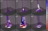 |
Fig. 1 Snapshots of the evolution of the system during the generation of a mild straight jet (top row) and a very energetic helical jet (bottom row) for the β = 0.025 simulation. The resp. [purple/pink] field lines, which are initially resp. [closed/open], are plotted from fixed points along the bottom boundary resp. [on a circle of radius 1.5L0/along the y = 0 axis]. The isosurface of the plasma density equal to |

The helical jet is unleashed by the explosive interchange reconnection between open and closed magnetic fields, which generates a series of impulsive nonlinear Alfvénic or kink waves that propagate upward along reconnection-formed open field lines (e.g., kinked purple in the bottom-middle panel of Fig. 1), and eject most of the twist (magnetic helicity) stored in the closed domain. The main acceleration process is explained by the untwisting model of Shibata & Uchida (1985, 1986), although a tension-driven flow is embedded within the structure of the helical jet (PAD09). In Sect. 5, we further study the physics and properties of the wave beyond that of our previous analysis.
In PDD15 we presented two parametric studies of the generation of straight jets and helical jets: one varied the inclination angle of the coronal magnetic field while the other varied the photospheric distribution of the magnetic field while preserving the basic topology. We confirmed that the basic model of PAD09 was valid across a broad parametric range. PDD15 showed that helical jets are triggered for inclination angles in the range θ = 0–20°. As long as a 3D magnetic null point is present, our model is also valid for different photospheric distributions of flux concentrations surrounding the central embedded-bipole polarity, configurations that are frequently observed in the solar atmosphere.
We showed in PDD15 that a helical jet was generated for all inclinations but this is not true for the straight jet. A straight jet formed only when the 3D null point was sufficiently stressed to form an extended current sheet in response to the boundary-driven motions. We found that straight jets appear only for inclination angles ≳8°. We also found that different photospheric magnetic distributions strongly affect the generation of the straight jet. From the first parametric studies presented in PDD15 we showed that a preceding reconnection-driven straight jet profoundly influences the onset of the succeeding helical jet. The third parametric study reported here will extend these results by showing that the actual occurrence of a straight jet is not essential, the early existence of intense reconnection is the key element that affects the trigger of the helical jet.
The parametric study presented here, however, goes further than merely confirming the results of PDD15. We present a completely new analysis of the underlying physical mechanism that accelerates the plasma in our model (Sect. 5). By varying β, we also show the original result that the morphology of the jet is strongly influenced by this parameter, a finding that was not expected from our previous simulations.
3. Model description
The simulations presented here extend the work presented in Pariat et al. (2015a, PDD15). In the simulations, we consider the equations of ideal magneto-hydrodynamics (MHD) for a monofluid coronal plasma of uniform density and temperature. The simulations were performed with the Adaptively Refined Magnetohydrodynamic Solver (ARMS), whose Flux-Corrected Transport algorithms are extensions of those derived in DeVore (1991). The time-dependent equations of ideal MHD, with the magnetic forces expressed in the Lorentz form, are solved on a dynamically solution-adaptive grid managed by the toolkit PARAMESH (MacNeice et al. 2000). This grid refines and derefines adaptively during the simulation as prescribed in the Appendix of Karpen et al. (2012). A Cartesian domain is assumed with x and y the horizontal axes and z the vertical axis. The simulation domain spans [−12L0;12L0] × [−12L0;12L0] × [0;24L0]. The nonuniform initial grid is identical to the one presented in Fig. 1 of PAD09. The same boundary conditions are used as in PDD15, i.e., line-tied at the bottom, closed on the four sides, and open at the top.
The initial magnetic field is set to be potential, using the specific analytical form given in Sect. 3 of PDD15. The initial configuration (cf. top-left panel of Fig. 1) is given by a central vertical magnetic dipole placed under the photosphere (producing a locally closed coronal field, e.g., purple lines in Fig. 1), embedded in an inclined (with respect to the vertical direction) and uniform background magnetic field (the open field, e.g., pink lines in Fig. 1). A 3D null point with its associated fan surface and two spine lines are present, with the outer spine following the general direction of the open field. In the present parametric study, the inclination angle θ = 10° is the same for all simulations. As in PDD15, energy is injected in the closed domain through line-tied twisting motions at the bottom boundary. The imposed velocity field is given by Eq. (3) of PDD15.
We follow the evolution of the free magnetic energy in the system, taken as the difference, Emag, between the total magnetic energy Em and its initial value: Emag(t) = Em(t)−Em(t = 0). This is only a proxy of the actual free magnetic energy, defined as the difference between the total magnetic energy in the system and the magnetic energy of the potential field having the same distribution of the normal magnetic field across the six boundaries. Although the system is initially potential and Bz at the bottom boundary is constant in time, since the magnetic flux distribution changes slightly on the other boundaries, the potential field and its energy change in time. Pariat et al. (2015b) showed in one case (their Fig. 2) that the difference between Emag and the real free energy is at most 20%, and that the two values are monotonically related.
The domain is filled with a highly conducting coronal plasma. For maximum generality, we use non-dimensional units (denoted as, e.g.,  ). The initial thermal pressure,
  , is uniform, as is the initial mass density,
  . We assume an ideal plasma equation of state. The temperature is therefore initially uniform,
  , where
  is the non-dimensional gas constant. The volume magnetic field
  is used as the reference magnetic field intensity. From this non-dimensional setting, choosing the value of certain physical quantities (denoted, e.g., f0) fully determines the physical scales of the system. The precise correspondence is detailed in Appendix A.
In this study, we analyse how modifying the plasma β impacts the development of the jet. All our previous published computations have been performed assuming β = 0.25, defined with respect to the uniform background field strength. In the present paper we performed three additional simulations where the β ranges from 1 to 2.5 × 10⁻³. We seek to test whether the modification of the β value precludes the existence of the jet, and to establish how it modifies the jet properties and dynamics.
The plasma β is varied by using different values for the non-dimensional plasma pressure . The simulations presented in PDD15 considered a value of uniformly equal to 0.01. We perform here additional runs with a uniform pressure in the domain, respectively equal to [4 × 10-2,10-2,10-3,10-4]. The non-dimensional density is kept constant between the runs,  , as is the volume magnetic field, . The plasma β is therefore given by
  . The different runs correspond to the respective plasma β values of [1.0,0.25,0.025,0.0025]. The non-dimensional Alfvén velocity,
  is therefore constant between the runs, which enables us to compare directly the evolutions of the four cases. The non-dimensional sound speed
  decreases with (and β), adopting the following values [0.26,0.13,0.041,0.013]. The parameters used in the four simulations are summarised in Table 1.
Characteristic of different simulations in non-dimensional units.
These four simulations enable us to simulate a wide variety of conditions in the solar atmosphere. The tables presented in Appendix A present various possible physical scalings that correspond to our different cases. The simulations using different values of β enable us more particularly to determine the dynamics of jets occurring in the different layers of the solar atmosphere. Table 2 presents one set of dimensional quantities that corresponds to different layers of the solar atmosphere for each run. The β = 0.025 and β = 0.0025 runs correspond to corona-like conditions, whereas the transition region would be typically represented with β = 0.25. The β = 1 run is applicable to some aspects of photosphere/chromosphere-like conditions. This correspondence is suggestive, but not definitive, since the chromosphere is a layer with strong density stratification while our simulations assume uniform ambient density. Due to the non-dimensional nature of the MHD system solved here, different β simulations can actually correspond to a wide range of parameters. As is shown in Appendix A, a given β simulation can apply to different layers for different values of the magnetic field, B0. The layer correspondence in Table 2 is only one possibility.
We note that our simulations focus on calculating the magnetically-driven dynamics of solar jets and not on the plasma thermal properties; consequently, we use a simple adiabatic energy equation and numerical resistivity. Our simulations do not include effects such as thermal conduction, or radiative transfer, or a generalised Ohm’s law with Hall and ambipolar-diffusion. These effects are well known to be important in the real corona and chromosphere for determining the plasma energetics (see e.g., Martínez-Sykora et al. 2012; Leake et al. 2013, 2014). Additionally, our simulations assume strict line-tying conditions at the lower boundary. The primary challenge in numerical simulation of solar jets, however is not the plasma thermodynamics, but the effective Lundquist number of the simulation. Even in the chromosphere the Lundquist number is high, >106 or so, well beyond the reach of present 3D simulations. It is absolutely essential that the numerical Lundquist number be as high as possible so that the resulting evolution is determined by true helicity-conserving reconnection rather than by simple diffusion. Our adaptive mesh refinement code ARMS does an excellent job at conserving helicity, even for reconnection-dominated evolutions (e.g., Knizhnik et al. 2015; Pariat et al. 2015b).
Possible scaling for the simulations.
4. Influence of the plasma beta on the trigger of straight and helical jets
In this section we examine how the plasma β influences the generation of the straight jet and helical jet. The morphology of the helical jet for each run is presented in Fig. 2, while the dynamical state of the system at t/t0 = 625, at the onset of the straight jet phase, is presented in Fig. 3. The evolution of the free magnetic energy, Emag (defined earlier in Sect. 3), and the kinetic energy, Ekin, for the runs at different β are presented in Fig. 4.
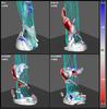 |
Fig. 2 Morphology of the helical jet during the blowout for simulations with different plasma β. The cyan field lines, which were all initially closed, are plotted from fixed points along the bottom boundary on a circle of radius 1.6L0. The helical jet in each simulation is highlighted by an isosurface of the plasma density equal to |
![Mathematical equation: \hbox{$\hat{\rho}=[1.05; 1.2; 1.6; 2.3]$}](/articles/aa/full_html/2016/12/aa29109-16/aa29109-16-eq117.png)
The first result is that, for all the values of β tested, a helical jet always occurs eventually. Figure 2 shows the existence of a higher-density/higher-temperature region related to helical upflows and the presence of an upward propagating nonlinear Alfvénic wave, as first introduced in PAD09 and discussed further in Sect. 5 below.
We observe in all runs that the jet consists of a left-handed helical density structure. The specific density distribution (shown by the isodensity surfaces) in the different helical jets exhibits variations in the width and pitch of the helical density structure, which we discuss further in Sect. 6. All of the simulations present a similar distribution of vx (red/blue color-coding of the isodensity surface) indicating plasma flowing away from the observer on the left side of the jet and toward the observer on the right. For each parametric run, this red/blue pattern on opposite sides of the jet characterises the strong clockwise rotation associated with the untwisting of the reconnected field lines.
The free magnetic and kinetic energy curves shown in Fig. 4 all follow the typical evolution observed previously (PDD15) during the generation of the helical jet. There is a peak of the free magnetic energy, followed by a sudden drop, corresponding to the release of magnetic energy by intense magnetic reconnection (top panel). The partial transformation of magnetic to kinetic energy results in a sharp peak in the latter (bottom panel). The changes in the free energy are proportional to the intensities of the kinetic energy, as shown in PAD10. Quantitative differences are observed among the different runs regarding the helical jet trigger, however: the trigger time and the free energy levels differ from one simulation to another. Using Eq. (5) of PDD15, we derive the trigger time, Ttrig, and the trigger energy, Etrig, from the peak of the free magnetic energy curves (Fig. 4, top panel). The resulting values are given in Table 3. We find consistently that for increasing values of β, the helical jet tends to occur later, after a greater amount of energy has been stored.
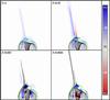 |
Fig. 3 Vertical velocity, vz distribution in the y−z plane at x = 0 at t = 625, during the straight jet/pre-helical jet phase for simulations with different plasma β highlighting the presence of a straight jet for the runs at higher β. The velocity magnitude is color coded in blue (upflows) and red (downflows). For comparison, the ambient Alfvén speed is ĉA = 0.28. The black field lines, all initially closed correspond to the cyan field lines of Fig. 2. Open black field lines for lower β runs indicate the occurrence of relatively more intense reconnection by this stage. The blue and green lines are isocontours of the electric current density. |
In PDD15, we observed that the straight jet developed before the onset of the helical jet for sufficiently large values of the inclination angle (θ > 8°). The present β = 0.25 run (with θ > 8°) hence also develops a straight jet with a higher-density region and marked upflowing vertical velocities aligned along the outer spine (upper right panel of Fig. 3). However, no similar straight jet is observed for the runs with lower values of β before the onset of the helical jet. For example, only a small upflow with a relatively limited vertical extent is observed in the β = 0.025 run (lower left panel of Fig. 3). Similar to the case β = 0.25, the straight jet is present for the β = 1 simulation. In the previous parametric simulations (cf. Fig. 4 of PDD15), we noted that the straight jet preceding the formation of the helical jet also was accompanied by an increase of the kinetic energy. Figure 4, lower panel, displays a similar behaviour (which was not observed in he axisymmetric case of PAD09).
The absence of a straight jet for the lower β runs does not mean that reconnection is absent in this phase. On the contrary, reconnection actually occurs in the lower β runs, as well. This can be noted first in Fig. 3 by the existence of longer and more intense current sheets: for smaller β, the length of the blue and green isocontours of the current density in the vicinity of the null point increases. In addition, for smaller β, one observes that some black field lines are open, whereas they initially belonged to the closed domain. Furthermore, we observe in Fig. 4 that the lower-β curves of the free magnetic energy present a slightly more gentle slope, an indication of the magnetic dissipation occurring at the reconnection site. This demonstrates that relatively more reconnection has occurred at t/t0 = 625 for the runs with smaller β, even though the driving is the same.
By analysing the moment at which the intense current sheet appears (not shown here), we find that the lower the β, the earlier the current sheet forms at the 3D null point, and the more intense is the reconnection when it develops. This indicates that the lower the plasma β, the earlier and the stronger is the reconnection during the straight jet phase. However, in our low-β simulations, this more intense reconnection does not result in the formation of a more marked high-density region and extended upflows that would be interpreted as an straight jet. In the high-β regime, reconnection may more efficiently produce high-density upflows, while at lower β, although more magnetic energy is released by reconnection, this energy does not drive high-density plasma flows.
A possible physical origin of this result may be related to our assumed initial conditions. We note that the initial state has a static, uniform density and temperature plasma and a potential magnetic field. Consequently, if interchange reconnection were to occur very easily, for example as soon as the photospheric driving is turned on, no straight jet would be observed, because the closed plasma released by the reconnection would have identical properties to the open. Furthermore, the nonlinear Alfvén wave flux produced by the reconnection would be minimal. In order for the interchange reconnection to produce an important effect, the closed flux must undergo a substantial deformation with a large current sheet built up at the deformed null and a compression of the closed plasma against the dome-like separatrix. This result re-emphasises the point raised above on the critical importance of the effective Lundquist number of the simulation. We find that, for very low plasma β, interchange reconnection begins so easily that the released closed plasma is near its initial state. It should be noted, however, that in the real corona the plasma in closed field embedded bipoles generally has higher temperature and density than surrounding open field plasma. In this case any interchange reconnection, even for very low β, would result in an observable straight jet. However, our basic result is still valid, the higher the β the higher the density of the released plasma (compared to its initial state).
As noted earlier, for higher β, the helical jet is generated later and after a greater amount of energy has been stored. Thus, there is a correlation between the low values of β, the important reconnection in the straight jet phase (whether or not a straight jet is actually present), and the earlier and lower energy trigger of the helical jet. In PDD15, our parametric studies of the field inclination and the photospheric flux distribution demonstrated that more intense reconnection in the pre-helical-jet phase (e.g., during the straight-jet phase) was correlated with an easier trigger of the helical jet, at lower energy and earlier in time. This third parametric study of the plasma β further confirms our previous findings: the reconnection during the straight jet phase strongly influences the timing and energetics of the helical jet phase. Our current results suggest, with respect to our other parametric study, that it is not the plasma β that directly triggers the helical jet at a lower energy threshold, but rather the intermediate action of reconnection developing during the straight jet phase, prior to the helical jet onset. A stronger current sheet at the null and more intense reconnection during the straight jet phase trigger the helical jet earlier and at a lower stored-energy level.
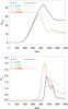 |
Fig. 4 Top panel: time evolution of the free magnetic energy, Emag, for simulations with different plasma β. Bottom panel: time evolution of the kinetic energy, Ekin, in each simulation. |
Why reconnection is stronger at lower β can be partly understood by the important growth of the closed domain for the lower-β runs. As discussed in PDD15, the reconnection at the 3D null during the straight jet phase is driven by the magnetic forcing imposed at the bottom boundary. While the amount and rate of energy injection is exactly the same in all runs, the plasma reacts differently to the driving depending on β. Indeed, the increase in the magnetic pressure imposed by the twisting is more strongly compensated by the plasma pressure at higher β. The higher the β, the less the closed-field domain bulges as a consequence of the twisting. This can be observed in Fig. 3, where the closed domain (distinguished by the black field lines) occupies a larger volume for lower value of β. The growth of the closed domain induces a stress on the 3D magnetic null point. The more the closed domain bulges, the more stressed is the 3D magnetic null point, and the faster reconnection develops. This explains why, during the straight jet phase, the reconnection is stronger for lower values of β, as the magnetic reconnection is more easily forced. Then, as the reconnection is stronger for lower values of β, it leads to an easier helical jet generation, as seen in previous parametric simulations.
Overall, the trigger and driver of the helical jet are similar in all runs, while the intensity of the straight jet depends sensitively on the value of β. The coronal jet model of PAD09, PAD10, and PDD15 generates helical jets for a wide range of plasma β. The helical jets for β of magnitude 10-2 and 10-3 are very similar. Hence, we argue that our jet model would also act similarly at still smaller values of β, as the influence of the plasma pressure becomes even more negligible. Overall, therefore, the model is able to produce multiple types of helical jet-like events that are observed to occur in the various layers of the solar atmosphere (cf. Sects. 1 and 7).
5. Driver of the helical jet
As discussed in the Introduction, previous studies have suggested that helical jets were driven/accelerated by untwisting upflows thanks to propagating nonlinear waves. In the present section, we further study how the untwisting model can drive the plasma upward and form the helical structure of the jet in different β environments.
Figure 5 presents the time evolution of the vertical (vz) and horizontal (v⊥) components of the plasma flow along the vertical direction at a given point (x,y) in each β simulation. The time slice shows the upward propagation of an enhanced velocity structure for both components. In this figure, we note the propagation front of the upward-moving wave and compare it to the local plasma flow speeds. We recall that the Alfvén speed is constant (cA = 0.28), while the sound speed, cS, decreases with smaller β (cf. values in Table 2). The wave character of the jet is immediately apparent in the discrepancy between the phase speed and the bulk speed of the plasma for the three lowest-β simulations. The wave propagates upward at near-Alfvén speed, i.e., vϕ ≈ [0.26,0.22,0.25] respectively for the β = [0.25,0.025,0.0025] runs, which represents [93,78,89] % of the large-scale Alfvén speed and [2.0,5.4,19.2] times the global sound speed, respectively. The phase speed of the propagating wave is Alfvénic and strongly supersonic. In these simulations, the actual vertical bulk speed of the plasma, vz, shown color-coded in the left column of Fig. 5, is significantly smaller than cA, with maximum values not exceeding 0.14 for z> 8 (higher velocities can be observed elsewhere, in particular around the reconnection site). The horizontal speed, v⊥, is roughly the same for the three low-β simulations.
The β = 1 simulation differs from the others. In that run, the speed of the upward propagating front is vϕ ≈ 0.17; this is lower than in the other cases and, most importantly, corresponds to the vertical bulk speed of the plasma. In this case, the upward motions correspond to the bulk flow of the material, and the flow is much slower than the large-scale Alfvén and sound speeds (here cS = 0.26).
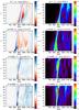 |
Fig. 5 Time evolution of the vertical and horizontal velocities (respectively vz and v⊥) along the vertical direction z at particular points (x,y), in units of L0, in the four simulations at different β. The phase velocity vϕ of the propagating wave is indicated by dashed lines. For comparison, the ambient Alfvén speed is ĉA = 0.28. |
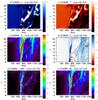 |
Fig. 6 Time evolution of the plasma density, ρ, temperature, T, vertical and horizontal velocities (respectively vz and v⊥), magnitude of the Lorentz Force, | j × B |, and Alfvén Mach number, MA, along the vertical direction z at a particular points (x,y), in units of L0, in the β = 0.0025 simulation. The phase velocity vϕ = 0.25 of the propagating wave is indicated by bright dashed lines, while the bulk speed of material transport at vz = 0.04 is indicated by darker dashed lines. For comparison, the initial uniform density is |

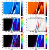 |
Fig. 7 Time evolution of the plasma density, ρ, temperature, T, vertical and horizontal velocities (respectively vz and v⊥), magnitude of the Lorentz Force, | j × B |, and Alfvén Mach number, MA, along the vertical direction z at a particular points (x,y), in units of L0, in the β = 1 simulation. The phase velocity vϕ = 0.15 of the propagating wave is indicated by bright dashed lines. For comparison, the initial uniform density is |
To examine the differences further, Figs. 6 and 7 present time slices of different quantities for the β = 0.0025 and β = 1 simulations, respectively. Figure 6 shows the upward displacement of a region of enhanced density and temperature that traces the jet in the β = 0.0025 simulation. The 1D cut is located at (x,y) = (0,−3.2)L0 which is roughly at the distance of the photospheric separatrix between the closed and open fields. Relative to Fig. 2, bottom left panel, this vertical cut is located at roughly the same distance from the center than the open cyan field lines, and is passing through the high density branch of the helical jet which is on the side of the viewer. This branch corresponds to the high density region at t = 875, z ~ 12, in Fig. 6, top left panel. The panels display structures propagating at two different speeds. First, a propagation front is present with a speed of 0.25, corresponding to the propagation of the nonlinear torsional Alfvén wave. This front spatially corresponds to an enhanced perpendicular velocity, to a strong Lorentz force | j × B |, and to a local Alfvén Mach number, MA (the ratio of the local momentum to the local Alfvén speed), close to 1. The surrounding field not having been previously perturbed, the local Alfvén speed equals the general large-scale value of ĉA = 0.28, at the moment of the passage of the wave. While the wave propagates upward close to the local-Alfvén speed, its associated plasma motions attain the local Alfvén speed, as shown by the values of MA close to unity. The driver of the upward flows is the Lorentz force. The tension of the kinked magnetic field line creates an upward and rotating force which accelerates the plasma. Its action may be qualitatively understood by the analytical model of Shibata & Uchida (1985, cf. Sect. 3 of that study). The wave propagates upward at a speed several times higher than the bulk flow of the plasma. The plasma, which has been accelerated by the passage of the torsional wave, then propagates upward trailing the wave. This explains the second type of structure observed in the time-slice plots of the density and temperature. In the wake of the propagation front, we observe that the high-density and -temperature region moves upward with a speed of 0.04, which corresponds to the local plasma velocity.
For the three low-β simulations, the jet dynamics result from the action of these two components, the wave propagation and the plasma upflows. Along each reconnected field line, the helicity and twist are redistributed and a nonlinear wave is generated. The propagating torsional Alfvén wave accelerates, heats, and compresses the plasma, giving it a rotating helical shape. Then, the structure evolves in the wake of the wave, due to the flow speed imparted to the plasma. The overall 3D morphology of the untwisting model is the result of these processes developing at multiple points in the domain along the sequentially reconnecting magnetic field lines.
In the β = 1 simulation, while the main driver remains the propagating torsional Alfvén wave, the situation is a bit simpler. The 1D cut is located at (x,y) = (0,0.1)L0 close to the center of the domain. Relatively to Fig. 2, top left panel, this cut is passing in the middle of the open cyan field line and passing through high density region of the helical jet. The jet is here formed by a bulk flow co-spatial with the wave. Figure 7 shows that the upward displacement of the enhanced-density and -temperature region progresses at the local vertical speed of the plasma, here around 0.15. The jet is thus solely the resultant of an upward bulk flow. The jet rotates with a transverse speed in the same range as the vertical speed. As in the low-β runs, the jet is nonetheless magnetically driven. This is demonstrated by the fact that the upward-moving material propagates at the local Alfvén speed, as shown by the value of the Alfvénic Mach number, MA, which is markedly high at the location of the jet, close to unity in the bottom part and slightly decreasing (>0.6) as the jet progress further up. Furthermore, the jet is directly cospatial with a region of strong Lorentz force, | j × B |. Hence, the driver of the jet in this case is again the magnetic torsional wave. For this β = 1 run, the wave accelerates the bulk of the plasma at the same speed as the phase speed of the wave. The helical jet structure, as shown in Fig. 2, here directly corresponds to and maps the propagating torsional wave.
6. Morphology of the helical jet
The variations in β have another important consequence for the dynamics of the untwisting model. The morphology of the helical jet is indeed strongly influenced by β. This is, of course, partly due to the differences in the driving properties studied in the previous section. In addition, there are differences in the dynamics at the reconnection site, as discussed in this section.
Beyond the trigger time and energy already defined in Sect. 4, from the 3D data of the time evolution of the thermodynamic quantities, we can derive other properties of the jets in the different runs, such as its width, R, and its duration, Δt. To do this, we must first define the boundary of the jet within the continuous 3D distribution. For each simulation, we have defined corresponding threshold values of the density, ρt, and temperature, Tt. These values correspond to regions of steep gradients of the corresponding quantities and define clearly the region of increased density and temperature that contains the jet. The values used for each run are listed in Table 3. The jets presented in Fig. 2 were plotted using the corresponding value of ρt. During the estimation of the different quantities presented hereafter, we checked that they only were minutely affected by reasonable variations of the precise values of ρt and Tt. In particular, different threshold values of ρt and Tt, to within a factor of 2, only marginally changed the estimated quantities. The measurement error bars provided in Table 3 are the outcomes of these two tests.
The choice of the values of ρt and Tt is, however, strongly influenced by the plasma β. Indeed, the pressure, density, and temperature excesses in the jet at lower β are relatively greater than in the higher-β runs. This is a direct consequence of the stronger impact of the magnetic field on the plasma in the lower-β environments. The helical jet is the result of the compressive effect of the propagating nonlinear Alfvénic wave. While the Lorentz force in the kinked part of the field lines has a constant magnitude between the different cases, its impact on the plasma dynamics is relatively stronger when β is smaller, i.e., it induces a stronger pressure increase at lower plasma β. Following an adiabatic ideal gas evolution, the plasma becomes denser and hotter. At lower β, the system can therefore more efficiently generate a jet that is dense and hot relative to the surrounding environment. Therefore, our model predicts that the plasma properties observed in the jet will depend sensitively upon the plasma β environment and, hence, on the layer of the atmosphere in which the jet is generated (see Sect. 7). It should be emphasised here that this conclusion is only true for the helical jet driven by the expolosive burst of interchange reconnection. As discussed above, the early-phase straight jet exhibits the opposite variation with plasma β.
Characteristics of the helical jets in the parametric β simulations.
It is evident from Fig. 2 that while all the jets present a rotating helical structure, the characteristics of the helix vary with β. The lower β is, the wider is the jet, i.e., the greater is the amplitude of the helix. For β = 1, the spire of the jet is compact and the jet appears as a thin and very collimated structure. In the case of the low-β runs, the jets present a much wider structure similar to a rotating hollow cylinder or a “cylinder with helical structure on the surface” as described in Shen et al. (2011). The half-width of the jet, i.e., the amplitude of unwinding helical global wave, is taken as the radius of the hollow cylinder, R, given in Table 3. The ratio of R to the characteristic size of the closed domain (the radius of the fan separatrix at the bottom boundary, equal to 2.2) is respectively on the order of [1.1,1.2,1.4,1.4] from higher to lower β. While the β = 1 helical jet appears narrower, it is nonetheless moving transversely across the domain. The whole structure is dynamically displaced horizontally over a distance comparable to the scale of the closed domain. This is likely due to the fact that the β = 1 jet is more directly advected by, or embedded with, the propagating wave: as the reconnection site moves sideways, so does the jet structure.
We also estimate the duration of the jet, Δt/t0, by inspecting the period during which a jet structure (with ρ ≥ ρt and T ≥ Tt is present in the simulated data (e.g., as in PAD09, cf. their Figs. 4 and 5). The obtained values are listed in Table 3. As was done for R, the error bars are derived from the results using the different threshold values of density and temperature. The variations in jet duration between the different runs can also be estimated from the energy plots presented in Fig. 4. Overall, one notes that the jets tend to last longer for lower values of the plasma β, with the β = 1 jet being markedly briefer than the three other cases.
In Table 3, we also list the average velocities measured in the jet for the different runs. The vertical velocity, ⟨ vz ⟩, roughly corresponds to the axial velocity along the direction of the jet (accounting for the inclination angle of 10° only modifies these values very slightly). The characteristic transverse velocity, ⟨ v⊥ ⟩, is taken to be the characteristic velocity in the xy plane in the middle of the jet (i.e., for z> 8). To determine these average values, we took the mean of the values of the velocity, restricted to the 3D sub-volume of high density and high temperature that defines the jet (i.e., using the threshold values in density, ρt, and temperature, Tt, defined above). We checked that varying the density, the temperature, or the combination of the two does not change significantly the derived values of the average velocities. As with R and Δt, the measurement error bars provided for the average values are the outcome of the different tests varying ρt, and Tt.
The total velocity of the plasma, ⟨ vplas ⟩, in Table 3 is the quadratic sum of the two velocities and corresponds to the bulk flow of the plasma. The jet phase velocity, vϕ, is taken as the vertical speed of the propagation front of the nonlinear Alfvénic wave, i.e., its phase speed, as estimated in Sect. 5.
We note that the (non-dimensional) perpendicular average velocity, ⟨ v⊥ ⟩ in the jet is relatively constant for all the runs, equal to ≈0.08, while ⟨ vz ⟩ decreases by a factor of 2 from the highest-β to the lowest-β simulation. These average values correspond to the mean velocities of the plasma within the whole jet structure, and thus are significantly smaller than the maximum values observed in Fig. 5. For the high-β run, the average velocities are higher as the jet is co-spatial with the Alfvénic torsional wave. For the low-β runs, in contrast, the average values are dominated by the velocities of the plasma after it has been accelerated by the nonlinear wave. In any case, the phase velocity of the jet, vϕ, is much greater than the plasma velocity in all the runs. Apart from the β = 1 run, vϕ is above 0.8cA. Both vϕ and ⟨ vplas ⟩ only appear to depend very weakly upon cS, especially in the β = 0.25 to 0.0025 range.
From the estimated average transverse velocity, ⟨ v⊥ ⟩, radius, R, and jet duration, Δt, we can derive the non-dimensional angular velocity of the rotation within the jet, ωt0, the pitch of the helical structure, h/L0, and an estimate for the numbers of turns in the jet, ΔN, from its morphological properties: 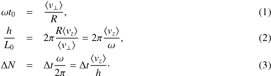 These estimations of the properties of the jet are regularly done in observed cases (e.g., Hong et al. 2013). We treat our data in a similar way, which permits a direct comparison between the properties of the present simulated jets with observed jets, as discussed in Sect. 7.
We observe that the non-dimensional angular speed ωt0 tends to decrease with decreasing β. Since the transverse average jet speed, ⟨ v⊥ ⟩, tends to be constant, this is mostly an effect of the larger width of the jet. We note that the non-dimensional pitch angle, h/L0, also tends to decrease with decreasing β (however, observe the more important uncertainty in these values). As noted earlier, this pitch-angle change is also verified by a visual inspection of the morphological shape of the jet (see Fig. 2). The higher the β, the thinner and less helical the jet appears. From the output of the simulations, we note that the density structure is rotated by half a turn along a height of 14 units for the β = 1 jet and of 8 units in the β = 0.0025 case. The variation in the pitch angle is mainly determined by the ratio ⟨ vz ⟩ / ⟨ v⊥ ⟩. Since the higher-β simulations are relatively more efficient at accelerating the plasma upward, compared to the transverse acceleration, these jets appear more pitched.
Excluding the β = 1 run, we note that the ejected twist ΔN inferred from the rotation is roughly constant for the runs at lower β and equal to ≈1.2. This value for ΔN is fully consistent with the amount of twist/helicity injected in the system by the boundary motions, which is on the order of 1.2 turns (cf. Sect. 3 in PDD15). As in PAD10, we also note that here the system appears quasi-potential after the jet occurs, i.e., only low-lying field lines next to the inversion line in the closed domain remain twisted. As noted in PAD09, for the lower-β runs, the reconnection at the 3D null during the jet removes most of the helicity by transferring it to the open field. In Pariat et al. (2015b), we measured that 90% of the helicity was eventually removed from the closed system. The amount of twist that we derive here from the observed rotation in the helical jet is fully consistent with this picture. We emphasise that the derivation of the twist from the rotation of the jet is completely independent of the magnetic field measurements. It indicates that, in observational cases, the derivation of azimuthal velocities assuming a cylindrical structure can be used to estimate the amount of twist stored initially.
It is interesting to note that, at any given time, the helical jet never displays a full rotation (e.g., Fig. 2 and other figures in previous studies). It only is the time-integrated observation of the jet evolution that enables one to infer the stored twist. This can be qualitatively understood since only about half of the twist contained on the closed field lines is eventually transferred to the open field lines when they reconnect. Consider a closed field line with a total twist τ: if this field line reconnects with the open field in its middle, only τ/ 2 will be acquired by the newly formed open field line and ejected. The other half of the twist will remain behind on a newly formed closed field line. Such field lines can later reconnect and transmit, for example, twist τ/ 4 to the open field. Hence, at any given time, only a fraction of the total stored helicity is given to the reconnected field lines. It only is due to the continuous and sequential reconnection that the newly open field lines extract nearly all the helicity from the closed field. The ability of the reconnection site to move within the 3D volume and reconnect most of the twisted flux enables the most efficient release of the helicity and energy. In the lower-β runs, we indeed observe that the reconnection site moves dynamically in the 3D space, hence more field lines sequentially reconnect, in some cases multiple times. The jets have thus a longer duration and their final free energy is notably lower, as can be noted from Fig. 4, compared to the β = 1 case.
For the β = 1 run, the amount of twist derived from the rotation is significantly smaller (ΔN ≈ 0.9), even though the helical jet was triggered later than in the other runs and, hence, after a greater amount of helicity has been stored (≈0.1–0.2 turns more). Thus, the β = 1 system releases much less helicity and energy than the other cases, as indicated by the greater amount of free energy remaining in the system (cf. Fig. 4) compared to the other runs. It can also be noted visually (not shown here) that many more twisted field lines are still present in the β = 1 system at the end of the helical jet phase. Here again, the measurements of the rotation speed in the jet enable a quantitative estimate of the amount of helicity ejected. The smaller value of ΔN indicates that, for β = 1, the system is much less efficient at releasing helicity compared to the other runs. We observe that the reconnection site moves less in the 3D space compared to the lower-β simulations. This is probably a consequence of the plasma resisting more strongly the rotation of the reconnection site, for β = 1. Because of the stronger plasma pressure, the 3D null point is not able to move as easily in the domain, and the reconnection of the twisted field lines over a large volume is inhibited. The reconnection site accesses less twisted flux, less flux can reconnect, and thus less helicity and free energy are removed from the closed system.
The stronger impact that the magnetic field has at lower β is thus the likely reason for the different morphology of the jet. The shape of the helical jet is the combined consequence of, first, the sequential interchange reconnection of the twisted field lines and, second, the ability of the propagating nonlinear Alfvénic wave to compress and accelerate the plasma (as discussed in Sect. 5). The helical structure is induced by the displacement of the reconnection site in the 3D volume. However, the extension of the current sheet, its rotation, and the displacement of the reconnection site are less easily achieved as the plasma β increases and the plasma is better able to resist the magnetic forces. Comparing the dynamics of the current sheet in the different simulations indeed shows that the current sheet is less extended and rotates over a smaller portion of the 3D domain for higher values of β. Consequently, the sequentially reconnected field lines remain in a smaller volume for higher β and the jet appears more compact. In contrast, for lower β the reconnection site is displaced over a very large domain. This leads to the reconnection of field lines farther away from the center of the configuration and creates a jet with the shape of a helical hollow cylinder or curtain, as observed in Fig. 2.
7. Conclusion
We further explored the physics of a model for the generation of solar jets (Pariat et al. 2009, PAD09). We have presented a parametric study of the influence of the plasma β parameter that extends our previous parametric studies of inclination angle and photospheric flux distribution (Pariat et al. 2015a, PDD15). We have confirmed that the model of PAD09 is robust, and can lead to the generation of both straight jets and helical jets, for a wide variety of uniform atmospheric conditions with β ranging from 10-3 to 1. We observed that the dynamics of the jets at β = 0.025 are very similar to those at β = 0.0025. We thus expect that this model is also working for values lower than 10-3, hence for any values of β ≤ 1. The model presented here is thus potentially able to explain jet-like events occurring in all the different layers of the solar atmosphere where the standard conditions for the validity of MHD are met.
While our model, based on a fully ionised single-fluid plasma with no atmospheric stratification, can properly represent large-scale coronal events, by no means does it completely represent the physics of jets that develop in the lower layers of the solar atmosphere. The fact that our jet model is able to produce helical jets for a wide range of β is important, given that helical structures are observed at many different scales in the various layers of the solar atmosphere. As discussed in the Introduction, twist and other signatures of rotating motions have been ubiquitously observed in jet-like events from the photosphere to the corona (e.g., Patsourakos et al. 2008; Curdt & Tian 2011; De Pontieu et al. 2012; Tian et al. 2014; Cheung et al. 2015). Our study suggests that a universal mechanism could potentially explain the helical properties observed in all types of solar jet-like phenomena. This mechanism, the generation of untwisting upflows induced by sequential reconnection and driven by propagating torsional Alfvénic waves, appears to fit multiple observed properties of the large-scale coronal jets, and could likely contribute to the similar dynamics observed in spicules and chromospheric jets. This idea, however, must be tested and evaluated using more complete numerical models of the photospheric and chromospheric layers (e.g., Martínez-Sykora et al. 2009, 2011, 2013; Kitiashvili et al. 2013; Takasao et al. 2013; Yang et al. 2013).
We have observed that varying the plasma β modifies the efficiency of the forcing of the driving motion on the 3D null point. Smaller β values lead to more efficient forcing of the 3D null, since the greater volume expansion of the closed domain induces earlier and stronger reconnection. However, at low β this does not necessarily induce a high-density outflow, and the straight jet is actually weaker at lower values of β. Although the reconnection is stronger at lower β, the straight jet is more marked at higher β (Sect. 4).
Our results concerning the trigger of straight jets and its influence on the generation of helical jets (Sect. 4) thus confirm and supplement the main conclusion drawn in PDD15 (summarised in Sect. 2 of the present study). Whether or not the straight jet is actually observed during the pre-helical-jet phase, at lower plasma β we note a higher amount of reconnection during the pre-helical-jet phase associated with an earlier trigger of the helical jet. Similar to the results obtained from the two previous parametric simulations of PDD15, we note that the occurrence of strong reconnection during the pre-helical-jet phase has an important impact on the trigger of the helical jet. Thanks to the present parametric simulation, we note that the presence of a high-density outflow (the straight jet) is not the determinant factor; rather it is the occurrence of reconnection prior to the helical jet. We confirm that the stronger is the reconnection during the straight jet phase, the lower is the energy/helicity threshold for triggering the instability of the helical jet, i.e., the easier it is to generate the untwisting upflows. As discussed in the conclusion of PDD15, this result is very revealing for the instability leading to the trigger of helical jets.
The parametric study carried out here, however, provides original results that go beyond the results of PDD15 and previous studies. It highlights for the first time the direct impact of the plasma β on the morphology and plasma properties of the helical jet (Sect. 6). At lower β, the jet assumes the shape of a high-density helix on the surface of a hollow cylinder. For β ≈ 1, the jet is much more compact and much more collimated, but nonetheless exhibits a dynamic transverse displacement in the domain. Its “Eiffel Tower” shape is more distinct. Higher β induces a smaller width of the global cylindrical volume and a shallower helical pitch angle. Jet at higher β thus appear more collimated than at lower β. Low-β helical jets also have a higher relative density and temperature compared to their environment.
Apart from the β = 1 case, the amount of twist ejected only is weakly influenced by the plasma β. The 3D null point is always able to efficiently eject a substantial amount of magnetic helicity, on the order of one turn of the magnetic field. Several observational studies have investigated in detail the kinematics of the jet plasma (Sect. 1). Assuming a cylindrical rotation, the jet radius, R, the transverse velocity, vt, the rotation rate, ω, and the number of turns, ΔN, have been derived in observational cases, in a way similar to our derivations of these quantities in Sect. 6. Interestingly, the published results are very consistent independent of the scale. From the amplitude of the motion and the transverse velocity observed in a chromospheric jet (Liu et al. 2009, their Fig. 4), a rotation rate of ω ≈ [0.011–0.025] rad s-1 of the untwisting structure was deduced. For a large coronal blowout jet, Shen et al. (2011) found a rotation rate ω ≈ 0.011 rad s-1 and an ejected twist ΔN ≈ [1.2–2.5] turns. Chen et al. (2012) estimated ω ≈ [0.01–0.015] rad s-1 while Hong et al. (2013) obtained ω ≈ 0.014 rad s-1 and ΔN ≈ 0.9 turns. Cheung et al. (2015, cf. Fig. 5) analysed a transition region jet with a width of about 10 Mm and transverse velocities above 50 km s-1, hence a rotation rate greater than 0.01 rad s-1. Using the scaling of t0 suggested by our Table 2, the equivalent dimensional rotation rate ω measured in our simulation ranges between 0.01 and 0.03 rad s-1, with an ejected number of turns ΔN ≈ [0.9–1.3]. The rotation inferred from our modeled helical jet, therefore, is very consistent with the properties of these observed jets.
The β = 1 case, which corresponds to the lower layers of the solar atmosphere, is significantly less efficient at removing magnetic helicity. Less twist is ejected and greater amounts of helicity and energy remain in the system following the jet. Previously, we showed that the 3D null-point configuration at the base of the present jet model readily allows the generation of recurrent homologous events (Pariat et al. 2010, PAD10). When subjected to a constant energy input, the system produces quasi-periodic jets. Here 3D null points can play the role of a magnetic “capacitor” and efficiently store free magnetic energy in the closed domain. Each jet corresponds to a phase of free-energy release, during which the system relaxed partially toward its minimum-energy state. When subjected to a constant energy input, the system is able to produce quasi-periodic jets. For the β = 1 runs, more energy/helicity/twist is left in the system; therefore the system remains closer to the instability threshold. If energy were continuously injected into this system, as in PAD10, we conjecture that jets would be generated at a much higher frequency for β = 1 than for lower β. This may explain the much higher occurrence rate of jet-like phenomena in higher-β environments. Assuming that β = 1 can, to some extent, model the generation of solar spicules, our results could explain the very high occurrence rate and recurrence of spicules compared to larger-scale jet-like events.
We have also introduced a new analysis of the physical mechanism driving the plasma in our simulation. The use of time-space diagrams enabled us to obtain a clearer understanding of the underlying driver of the untwisting upflows (Sect. 5). We confirmed previous results (Shibata & Uchida 1985, 1986; Canfield et al. 1996; Jibben & Canfield 2004; Török et al. 2009; Pariat et al. 2009; Lee et al. 2015) that the primary driver of the helical jets is the propagating nonlinear Alfvénic torsional wave that develops on the sequentially reconnected open field lines. Compared to previous studies, our parametric study revealed how the plasma β of the surrounding field could influence the properties of the untwisting model. We found that, at all β, the acceleration was due to the Lorentz force present in the kinked section of the newly reconnected open field lines. The Lorentz force induced a local acceleration of the plasma at a velocity close to the local Alfvén speed. As the field lines untwist, the propagation of the twist induces a vertical as well as an azimuthal motion of the plasma. In addition, the wave generates an adiabatic heating and compression of the plasma, with higher efficiency for lower values of β.
At β = 1, we noted that the accelerated plasma and the wave are embedded within each other, and the jet simply corresponds to a bulk flow of plasma. At lower plasma β, we observed that the propagation/phase speed of the wave was close to the ambient Alfvén speed, and was much higher that the bulk flow speed of the plasma. Once accelerated at the front of the propagating wave, the dense and hot plasma then moves independently of the wave at its own speed along the field lines. At low β, the overall morphology of the jet is thus distinct from the evolution of the kink present on the field lines.
As discussed in the Introduction, jets are likely generated by multiple acceleration mechanisms, including both the evaporation upflows and untwisting upflows. The coexistence of the evaporation and untwisting upflows implies multi-velocity observations in jet events. This can possibly explain the discrepancy between the average velocity measurements of coronal jets obtained from imaging instruments compared with those obtained from spectroscopy. Spectroscopic measurements, which enable estimates of the bulk flow of the plasma in jets (Kamio et al. 2007, 2010; Madjarska 2011; Young & Muglach 2014b,a), rarely found velocities higher than 300 km s-1. However, for the low-β cases, we stress that the untwisting mechanism, by itself, produces two types of velocities: a phase speed that we find to be close to the Alfvén velocity of the open field, and a bulk plasma flow that is only fraction of the phase speed. Velocity measurements obtained from imaging instruments, based on the estimation of a structure-front speed and, hence, more likely to measure the phase speed of a wave, frequently measure velocities higher than 500 km s-1 (Shimojo et al. 1996; Cirtain et al. 2007; Savcheva et al. 2007). The higher speeds measured by imaging techniques may simply reflect the higher phase speed of the helical jet wave front, compared to the much slower bulk plasma flows. The latter may be formed from either the evaporation upflows or the bulk-flow component driven by the untwisting mechanism, or both.
In summary, the results of our present analysis enables further understanding of the dynamics of jets developed in previous studies. The jet structure and dynamics are the result of the following processes. First, the 3D sequential reconnection of the closed, twisted field lines creates new open field lines with a large amount of twist close to the footpoint. For each of these new open field lines, the twist is then ejected through the generation of propagating torsional Alfvénic waves. The propagating wave heats and compresses the plasma as it propagates upward at its Alfvénic phase speed. The accelerated plasma can then eventually move along the field lines at the speed it acquired. While tension-driven motions are observed to be embedded within the helical jet structure, they only play a minor role in explaining the dynamics of the plasma. We reiterate that we do not treat any effects related to evaporation jets since our model does not include non-ideal plasma effects such as heat conduction or plasma pressure differences between the closed and open field, all of which can drive additional flows. A real jet is likely the combination of these different types of mechanisms that induce multi-thermal and multi-velocity features.
Thanks to the recent numerical studies of jets, understanding of the possible underlying jet mechanism has grown quickly. Using multi-wavelength EUV spectroscopic observations, Matsui et al. (2012) provided the interesting results that most of the velocities measured at higher temperature (T> 105.5 K) were consistent with evaporation upflows. On the other hand, emissions at lower temperatures were much higher than what is expected due to the evaporation mechanism. Since emission at these lower temperature tends to more frequently and more clearly display helical motions, this would suggest that it is mainly in this temperature range that the untwisting upflows mechanism that we are modeling here is dominant. In any case, the acceleration mechanism can only be understood fully if a complete diagnostic of the jet and surrounding plasma properties is performed. Spectroscopic measurements, such as those provided by the IRIS spacecraft (De Pontieu et al. 2014b), are the keys to advance our understanding of jet-like events in the different layers of the solar atmosphere.
Acknowledgments
The authors thank the referee for helpful comments which improved the clarity of the paper. The authors acknowledge access to the substantial HPC resources of CINES under the allocations 2014–046331, 2015−046331, and 2016–046331 made by GENCI (Grand Équipement National de Calcul Intensif). We also appreciate the support of the International Space Science Institute and the contributions by other team members during the workshops Understanding Solar Jets and their Role in Atmospheric Structure and Dynamics. K.D. acknowledges support from the Computational and Information Systems Laboratory and the High Altitude Observatory of the National Center for Atmospheric Research, which is sponsored by the National Science Foundation. C.R.D., S.K.A., and J.T.K. all gratefully acknowledge support from NASA’s LWS TR&T and H-SR programs.
References
- Antiochos, S. K. 1990, Soc. Astron. It., 61, 369 [NASA ADS] [Google Scholar]
- Archontis, V., & Hood, A. W. 2013, ApJ, 769, L21 [NASA ADS] [CrossRef] [Google Scholar]
- Canfield, R. C., Leka, K. D., Shibata, K., Yokoyama, T., & Shimojo, M. 1996, ApJ, 464, 1016 [NASA ADS] [CrossRef] [Google Scholar]
- Chen, H.-D., Zhang, J., & Ma, S.-L. 2012, Res. Astron. Astrophys., 12, 573 [NASA ADS] [CrossRef] [Google Scholar]
- Cheung, M. C. M., De Pontieu, B., Tarbell, T. D., et al. 2015, ApJ, 801, 83 [NASA ADS] [CrossRef] [Google Scholar]
- Chifor, C., Isobe, H., Mason, H. E., et al. 2008a, A&A, 491, 279 [NASA ADS] [CrossRef] [EDP Sciences] [Google Scholar]
- Chifor, C., Young, P. R., Isobe, H., et al. 2008b, A&A, 481, L57 [NASA ADS] [CrossRef] [EDP Sciences] [Google Scholar]
- Cirtain, J. W., Golub, L., Lundquist, L. L., et al. 2007, Science, 318, 1580 [NASA ADS] [CrossRef] [PubMed] [Google Scholar]
- Cranmer, S. R., & Woolsey, L. N. 2015, ApJ, 812, 71 [NASA ADS] [CrossRef] [Google Scholar]
- Curdt, W., & Tian, H. 2011, A&A, 532, L9 [NASA ADS] [CrossRef] [EDP Sciences] [Google Scholar]
- Curdt, W., Tian, H., & Kamio, S. 2012, Sol. Phys., 280, 417 [NASA ADS] [CrossRef] [Google Scholar]
- De Pontieu, B., Mcintosh, S. W., Carlsson, M., et al. 2007, Science, 318, 1574 [NASA ADS] [CrossRef] [PubMed] [Google Scholar]
- De Pontieu, B., Carlsson, M., Rouppe van der Voort, L. H. M., et al. 2012, ApJ, 752, L12 [NASA ADS] [CrossRef] [Google Scholar]
- De Pontieu, B., Rouppe van der Voort, L., Mcintosh, S. W., et al. 2014a, Science, 346, 1255732 [CrossRef] [Google Scholar]
- De Pontieu, B., Title, A. M., Lemen, J. R., et al. 2014b, Sol. Phys., 289, 2733 [NASA ADS] [CrossRef] [Google Scholar]
- Dere, K. P., Bartoe, J.-D. F., & Brueckner, G. E. 1989, Sol. Phys., 123, 41 [NASA ADS] [CrossRef] [Google Scholar]
- DeVore, C. R. 1991, J. Comput. Phys. 92, 142 [Google Scholar]
- Fang, F., Fan, Y., & Mcintosh, S. W. 2014, ApJ, 789, L19 [NASA ADS] [CrossRef] [Google Scholar]
- Harrison, R. A., Bryans, P., & Bingham, R. 2001, A&A, 379, 324 [NASA ADS] [CrossRef] [EDP Sciences] [Google Scholar]
- Hong, J.-C., Jiang, Y.-C., Yang, J.-Y., et al. 2013, RA&A, 13, 253 [Google Scholar]
- Jiang, Y. C., Chen, H. D., Li, K. J., Shen, Y. D., & Yang, L. H. 2007, A&A, 469, 331 [NASA ADS] [CrossRef] [EDP Sciences] [Google Scholar]
- Jibben, P., & Canfield, R. C. 2004, ApJ, 610, 1129 [NASA ADS] [CrossRef] [Google Scholar]
- Kaiser, M. L., Kucera, T. A., Davila, J. M., et al. 2008, Space Sci. Rev., 136, 5 [NASA ADS] [CrossRef] [Google Scholar]
- Kamio, S., Hara, H., Watanabe, T., et al. 2007, Publ. Astron. Soc. Japan, 59, 757 [Google Scholar]
- Kamio, S., Curdt, W., Teriaca, L., Inhester, B., & Solanki, S. K. 2010, A&A, 510, L1 [NASA ADS] [CrossRef] [EDP Sciences] [Google Scholar]
- Karpen, J. T., Antiochos, S. K., & DeVore, C. R. 2012, ApJ, 760, 81 [NASA ADS] [CrossRef] [Google Scholar]
- Karpen, J. T., DeVore, C. R., Antiochos, S. K., & Pariat, E. 2016, ArXiv e-prints [arXiv:1606.09201] [Google Scholar]
- Kitiashvili, I. N., Kosovichev, A. G., Lele, S. K., Mansour, N. N., & Wray, A. A. 2013, ApJ, 770, 37 [NASA ADS] [CrossRef] [Google Scholar]
- Knizhnik, K. J., Antiochos, S. K., & DeVore, C. R. 2015, ApJ, 809, 137 [NASA ADS] [CrossRef] [Google Scholar]
- Leake, J. E., Lukin, V. S., & Linton, M. G. 2013, Phys. Plasmas, 20, 061202 [NASA ADS] [CrossRef] [Google Scholar]
- Leake, J. E., DeVore, C. R., Thayer, J. P., et al. 2014, Space Sci. Rev., 184, 107 [NASA ADS] [CrossRef] [Google Scholar]
- Lee, E. J., Archontis, V., & Hood, A. W. 2015, ApJ, 798, L10 [NASA ADS] [CrossRef] [Google Scholar]
- Liu, W., Berger, T. E., Title, A. M., & Tarbell, T. D. 2009, ApJ, 707, L37 [NASA ADS] [CrossRef] [Google Scholar]
- Liu, C., Deng, N., Liu, R., et al. 2011a, ApJ, 735, L18 [NASA ADS] [CrossRef] [Google Scholar]
- Liu, W., Berger, T. E., Title, A. M., Tarbell, T. D., & Low, B. C. 2011b, ApJ, 728, 103 [NASA ADS] [CrossRef] [Google Scholar]
- MacNeice, P., Olson, K. M., Mobarry, C., de Fainchtein, R., & Packer, C. 2000, Comp. Phys. Commun., 126, 330 [Google Scholar]
- Madjarska, M. S. 2011, A&A, 526, A19 [NASA ADS] [CrossRef] [EDP Sciences] [Google Scholar]
- Martínez-Sykora, J., Hansteen, V., de Pontieu, B., & Carlsson, M. 2009, ApJ, 701, 1569 [NASA ADS] [CrossRef] [Google Scholar]
- Martínez-Sykora, J., Hansteen, V., & Moreno-Insertis, F. 2011, ApJ, 736, 9 [NASA ADS] [CrossRef] [Google Scholar]
- Martínez-Sykora, J., de Pontieu, B., & Hansteen, V. 2012, ApJ, 753, 161 [NASA ADS] [CrossRef] [Google Scholar]
- Martínez-Sykora, J., de Pontieu, B., Leenaarts, J., et al. 2013, ApJ, 771, 66 [NASA ADS] [CrossRef] [Google Scholar]
- Matsui, Y., Yokoyama, T., Kitagawa, N., & Imada, S. 2012, ApJ, 759, 15 [NASA ADS] [CrossRef] [Google Scholar]
- Moore, R., Sterling, A. C., Falconer, D. A., & Robe, D. 2013, ApJ, 769, 134 [NASA ADS] [CrossRef] [Google Scholar]
- Moreno-Insertis, F., & Galsgaard, K. 2013, ApJ, 771, 20 [NASA ADS] [CrossRef] [Google Scholar]
- Moreno-Insertis, F., Galsgaard, K., & Ugarte-Urra, I. 2008, ApJ, 673, L211 [Google Scholar]
- Morita, S., Shibata, K., Ueno, S., et al. 2010, Publ. Astron. Soc. Japan, 62, 901 [Google Scholar]
- Nishizuka, N., Shimizu, T., Nakamura, T., et al. 2008, ApJ, 683, L83 [NASA ADS] [CrossRef] [Google Scholar]
- Nishizuka, N., Nakamura, T., Kawate, T., Singh, K. A. P., & Shibata, K. 2011, ApJ, 731, 43 [NASA ADS] [CrossRef] [Google Scholar]
- Nisticò, G., Bothmer, V., Patsourakos, S., & Zimbardo, G. 2009, Sol. Phys., 259, 87 [NASA ADS] [CrossRef] [Google Scholar]
- Nóbrega-Siverio, D., Moreno-Insertis, F., & Martínez-Sykora, J. 2016, ApJ, 822, 18 [NASA ADS] [CrossRef] [Google Scholar]
- Pariat, E., Antiochos, S. K., & DeVore, C. R. 2009, ApJ, 691, 61 [NASA ADS] [CrossRef] [Google Scholar]
- Pariat, E., Antiochos, S. K., & DeVore, C. R. 2010, ApJ, 714, 1762 [NASA ADS] [CrossRef] [Google Scholar]
- Pariat, E., Dalmasse, K., DeVore, C. R., Antiochos, S. K., & Karpen, J. T. 2015a, A&A, 573, A130 [NASA ADS] [CrossRef] [EDP Sciences] [Google Scholar]
- Pariat, E., Valori, G., Démoulin, P., & Dalmasse, K. 2015b, A&A, 580, A128 [NASA ADS] [CrossRef] [EDP Sciences] [Google Scholar]
- Patsourakos, S., Pariat, E., Vourlidas, A., Antiochos, S. K., & Wuelser, J. P. 2008, ApJ, 680, L73 [NASA ADS] [CrossRef] [Google Scholar]
- Pike, C. D., & Mason, H. E. 1998, Sol. Phys., 182, 333 [NASA ADS] [CrossRef] [Google Scholar]
- Rachmeler, L. A., Pariat, E., DeForest, C. E., Antiochos, S. K., & Török, T. 2010, ApJ, 715, 1556 [NASA ADS] [CrossRef] [Google Scholar]
- Savcheva, A., Cirtain, J. W., De Luca, E. E., et al. 2007, Publ. Astron. Soc. Japan, 59, 771 [Google Scholar]
- Savcheva, A., Cirtain, J. W., De Luca, E. E., & Golub, L. 2009, ApJ, 702, L32 [NASA ADS] [CrossRef] [Google Scholar]
- Schmieder, B., Shibata, K., van Driel-Gesztelyi, L. L., & Freeland, J. M. 1995, Sol. Phys., 156, 245 [NASA ADS] [CrossRef] [MathSciNet] [Google Scholar]
- Shen, Y., Liu, Y., Su, J., & Ibrahim, A. 2011, ApJ, 735, L43 [NASA ADS] [CrossRef] [Google Scholar]
- Shen, Y., Liu, Y., Su, J., & Deng, Y. Y. 2012, ApJ, 745, 164 [NASA ADS] [CrossRef] [Google Scholar]
- Shibata, K., & Uchida, Y. 1985, Astron. Soc. Japan, 37, 31 [Google Scholar]
- Shibata, K., & Uchida, Y. 1986, Sol. Phys., 103, 299 [NASA ADS] [CrossRef] [Google Scholar]
- Shibata, K., Nakamura, T., Matsumoto, T., et al. 2007, Science, 318, 1591 [NASA ADS] [CrossRef] [Google Scholar]
- Shibata, K., Acton, L. W., Strong, K. T., et al. 1992, Publ. Astron. Soc. Japan, 44, L173 [Google Scholar]
- Shimojo, M., Hashimoto, S., Shibata, K., et al. 1996, Publ. Astron. Soc. Japan, 48, 123 [Google Scholar]
- Sterling, A. C. 2000, Sol. Phys., 196, 79 [NASA ADS] [CrossRef] [Google Scholar]
- Sterling, A. C., Harra, L. K., & Moore, R. 2010a, ApJ, 722, 1644 [NASA ADS] [CrossRef] [Google Scholar]
- Sterling, A. C., Moore, R., & DeForest, C. E. 2010b, ApJ, 714, L1 [NASA ADS] [CrossRef] [Google Scholar]
- Suematsu, Y., Ichimito, K., Katsukawa, Y., et al. 2008, First Results From Hinode, ASP Conf. Ser., 397, 27 [NASA ADS] [Google Scholar]
- Takasao, S., Isobe, H., & Shibata, K. 2013, Pub. Astron. Soc. Japan, 65, 62 [Google Scholar]
- Tian, H., DeLuca, E., Cranmer, S. R., et al. 2014, Science, 346, 1255711 [Google Scholar]
- Török, T., Aulanier, G., Schmieder, B., Reeves, K. K., & Golub, L. 2009, ApJ, 704, 485 [NASA ADS] [CrossRef] [Google Scholar]
- Török, T., Lionello, R., Titov, V. S., et al. 2016, EGU General Assembly 2016, held 17−22 April, 2016, in Vienna, Austria, 2692 [Google Scholar]
- Wang, Y.-M., & Sheeley, N. R. 2002, ApJ, 575, 542 [NASA ADS] [CrossRef] [Google Scholar]
- Wyper, P. F., & DeVore, C. R. 2016, ApJ, 820, 77 [NASA ADS] [CrossRef] [Google Scholar]
- Wyper, P. F., DeVore, C. R., Karpen, J. T., & Lynch, B. J. 2016, ApJ, 827, 4 [NASA ADS] [CrossRef] [Google Scholar]
- Yang, L., He, J., Peter, H., et al. 2013, ApJ, 777, 16 [NASA ADS] [CrossRef] [Google Scholar]
- Young, P. R., & Muglach, K. 2014a, Publ. Astron. Soc. Japan, 66, S12 [Google Scholar]
- Young, P. R., & Muglach, K. 2014b, Sol. Phys., 289, 3313 [NASA ADS] [CrossRef] [Google Scholar]
- Zeng, Z., Chen, B., Ji, H., Goode, P. R., & Cao, W. 2016, ApJ , 819, L3 [NASA ADS] [CrossRef] [Google Scholar]
- Zhang, Q. M., Chen, P.-F. F., Guo, Y., Fang, C., & Ding, M.-D. 2012, ApJ, 746, 19 [NASA ADS] [CrossRef] [Google Scholar]
Appendix A: Scaling of the MHD simulations relevant for solar-atmosphere like conditions
For a non-dimensional quantity, , derived by solving the numerical MHD equations, it is straightforward to derive the corresponding dimensional units f0 such that  , with fS a characteristic scale of that quantity. The scaling of the system is fully determined once the characteristic dimensional density ρ0, pressure P0, temperature T0, magnetic field B0, and length L0 are given. Assuming a given value of the plasma β and that the gas follows the ideal gas law, only two among ρ0, P0, T0, and B0 need to be specified. Indeed, these quantities are linked such that: with μ0 = 4π × 10-7 Wb A-1 m-1 the vacuum permeability and R0 the ideal gas constant scale. For a fully ionised plasma only composed of hydrogen, one has R0 = 1.650 × 10⁴ m2 s-2 K-1. Fixing two of the quantities ρ0, P0, T0, and B0, therefore, determines the other two. This also fixes the velocity scale, V0, since
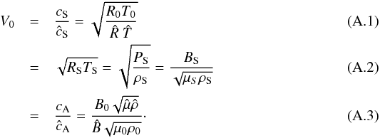
In order to close the system either the length scale, L0, or the time scale, t0, must be specified, the two being related such that L0 = V0t0.
In our numerical simulation, we use  , ,
, ,  and
and ![Mathematical equation: \hbox{$\hat{P} \in [4\times10^{-2},10^{-2},10^{-3},10^{-4}]$}](/articles/aa/full_html/2016/12/aa29109-16/aa29109-16-eq273.png) . The choice of determines the value of β. Then, fixing two of the quantities ρ0, P0, T0, and B0, as well as choosing either the length L0 or the time scale t0, fully determines all dimensions of the MHD system. The following Tables A.1–A.4 illustrate a wide range of possible systems that our simulations can represent. Table A.1 shows the effect of using different temperature T0; Tables A.2 and A.3 show the effect of using different volume magnetic field B0, fixing either the time scale or the length scale, respectively; and Table A.4 shows the effect of using different length scales, fixing P0 and T0 for each β.
. The choice of determines the value of β. Then, fixing two of the quantities ρ0, P0, T0, and B0, as well as choosing either the length L0 or the time scale t0, fully determines all dimensions of the MHD system. The following Tables A.1–A.4 illustrate a wide range of possible systems that our simulations can represent. Table A.1 shows the effect of using different temperature T0; Tables A.2 and A.3 show the effect of using different volume magnetic field B0, fixing either the time scale or the length scale, respectively; and Table A.4 shows the effect of using different length scales, fixing P0 and T0 for each β.
The quantities ρ0, P0, T0, B0 correspond to the values in the volume, away from the central polarity. The maximum field in the center of the polarity is equal to ≃14B0. The flux in the central polarity is ≃ . The null is at a height of ≃2.2L0, the polarity inversion line at ≃1.6L0, and the closed-domain separatrix at ≃3.4L0 from the center.
Possible scaling for the different plasma β simulations using constant volume magnetic field B0 (in G) and time t0 (in s), while varying the temperature T0 (in K).
Possible scaling for the different plasma β simulations using constant atmospheric temperature T0 (in K) and time t0 (in s), while varying the volume magnetic field B0 (in G).
Possible scaling for the different plasma β simulations using constant volume magnetic field B0 (in G) and length L0 (in Mm), while varying the atmospheric temperature T0 (in K).
Possible scaling for the different plasma β simulations using constant atmospheric pressure P0 (in Pa), while varying the temperature T0 (in K) and length L0 (in Mm).
All Tables
Possible scaling for the different plasma β simulations using constant volume magnetic field B0 (in G) and time t0 (in s), while varying the temperature T0 (in K).
Possible scaling for the different plasma β simulations using constant atmospheric temperature T0 (in K) and time t0 (in s), while varying the volume magnetic field B0 (in G).
Possible scaling for the different plasma β simulations using constant volume magnetic field B0 (in G) and length L0 (in Mm), while varying the atmospheric temperature T0 (in K).
Possible scaling for the different plasma β simulations using constant atmospheric pressure P0 (in Pa), while varying the temperature T0 (in K) and length L0 (in Mm).
All Figures
|
Fig. 1 Snapshots of the evolution of the system during the generation of a mild straight jet (top row) and a very energetic helical jet (bottom row) for the β = 0.025 simulation. The resp. [purple/pink] field lines, which are initially resp. [closed/open], are plotted from fixed points along the bottom boundary resp. [on a circle of radius 1.5L0/along the y = 0 axis]. The isosurface of the plasma density equal to |
| In the text | |
|
Fig. 2 Morphology of the helical jet during the blowout for simulations with different plasma β. The cyan field lines, which were all initially closed, are plotted from fixed points along the bottom boundary on a circle of radius 1.6L0. The helical jet in each simulation is highlighted by an isosurface of the plasma density equal to |
| In the text | |
|
Fig. 3 Vertical velocity, vz distribution in the y−z plane at x = 0 at t = 625, during the straight jet/pre-helical jet phase for simulations with different plasma β highlighting the presence of a straight jet for the runs at higher β. The velocity magnitude is color coded in blue (upflows) and red (downflows). For comparison, the ambient Alfvén speed is ĉA = 0.28. The black field lines, all initially closed correspond to the cyan field lines of Fig. 2. Open black field lines for lower β runs indicate the occurrence of relatively more intense reconnection by this stage. The blue and green lines are isocontours of the electric current density. |
| In the text | |
|
Fig. 4 Top panel: time evolution of the free magnetic energy, Emag, for simulations with different plasma β. Bottom panel: time evolution of the kinetic energy, Ekin, in each simulation. |
| In the text | |
|
Fig. 5 Time evolution of the vertical and horizontal velocities (respectively vz and v⊥) along the vertical direction z at particular points (x,y), in units of L0, in the four simulations at different β. The phase velocity vϕ of the propagating wave is indicated by dashed lines. For comparison, the ambient Alfvén speed is ĉA = 0.28. |
| In the text | |
|
Fig. 6 Time evolution of the plasma density, ρ, temperature, T, vertical and horizontal velocities (respectively vz and v⊥), magnitude of the Lorentz Force, | j × B |, and Alfvén Mach number, MA, along the vertical direction z at a particular points (x,y), in units of L0, in the β = 0.0025 simulation. The phase velocity vϕ = 0.25 of the propagating wave is indicated by bright dashed lines, while the bulk speed of material transport at vz = 0.04 is indicated by darker dashed lines. For comparison, the initial uniform density is |
| In the text | |
|
Fig. 7 Time evolution of the plasma density, ρ, temperature, T, vertical and horizontal velocities (respectively vz and v⊥), magnitude of the Lorentz Force, | j × B |, and Alfvén Mach number, MA, along the vertical direction z at a particular points (x,y), in units of L0, in the β = 1 simulation. The phase velocity vϕ = 0.15 of the propagating wave is indicated by bright dashed lines. For comparison, the initial uniform density is |
| In the text | |
Current usage metrics show cumulative count of Article Views (full-text article views including HTML views, PDF and ePub downloads, according to the available data) and Abstracts Views on Vision4Press platform.
Data correspond to usage on the plateform after 2015. The current usage metrics is available 48-96 hours after online publication and is updated daily on week days.
Initial download of the metrics may take a while.