| Issue |
A&A
Volume 595, November 2016
|
|
|---|---|---|
| Article Number | A129 | |
| Number of page(s) | 7 | |
| Section | Stellar atmospheres | |
| DOI | https://doi.org/10.1051/0004-6361/201628789 | |
| Published online | 16 November 2016 | |
Learning about stars from their colors
1 Instituto de Astrofísica de Canarias, Vía Láctea, 38205 La Laguna, Tenerife, Spain
e-mail: This email address is being protected from spambots. You need JavaScript enabled to view it.
2 Universidad de La Laguna, Departamento de Astrofísica, 38206 La Laguna, Tenerife, Spain
Received: 25 April 2016
Accepted: 21 September 2016
Abstract
Aims. We pose the question of how much information on the atmospheric parameters of late-type stars can be retrieved purely from color information using standard photometric systems.
Methods. We carried out numerical experiments using stellar fluxes from model atmospheres, injecting random noise before analyzing them. We examined the presence of degeneracies among atmospheric parameters, and evaluated how well the parameters are extracted depending on the number and wavelength span of the photometric filters available, from the UV GALEX to the mid-IR WISE passbands. We also considered spectrophotometry from the Gaia mission.
Results. We find that stellar effective temperatures can be determined accurately (σ ~ 0.01 dex or about 150 K) when reddening is negligible or known, based merely on optical photometry, and the accuracy can be improved twofold by including IR data. On the other hand, stellar metallicities and surface gravities are fairly unconstrained from optical or IR photometry: ~1 dex for both parameters at low metallicity, and ~0.5 dex for [Fe/H] and ~1 dex for log g at high metallicity. However, our ability to retrieve these parameters can improve significantly by adding UV photometry. When reddening is considered a free parameter, assuming it can be modeled perfectly, our experiments suggest that it can be disentangled from the rest of the parameters.
Conclusions. This theoretical study indicates that combining broad-band photometry from the UV to the mid-IR allows atmospheric parameters and interstellar extinction to be determined with fair accuracy, and that the results are moderately robust to the presence of systematic imperfections in our models of stellar spectral energy distributions (SEDs). The use of UV passbands helps substantially to derive metallicities (down to [Fe/H] ~ −3) and surface gravities, as well as to break the degeneracy between effective temperature and reddening. The Gaia BP/RP data can disentangle all the parameters, provided the stellar SEDs are modeled reasonably well.
Key words: techniques: photometric / stars: atmospheres / stars: fundamental parameters / dust, extinction
© ESO, 2016
1. Introduction
The border between photometry and spectroscopy is poorly defined. As soon as two photometric measurements, a color, are available, photometry can be considered as very-low resolution spectroscopy. Multicolor photometric systems are now evolving from a few passbands to dozens of contiguous narrow windows (see, e.g., Aparicio Villegas et al. 2010). Obviously, narrower and more numerous passbands covering a wider spectral range are desirable, but the information content does not necessarily increase linearly with the number of filters.
Bailer-Jones (2004) performed an optimization exercise varying the number, width, and location of the passbands to maximize the information content for stellar sources and minimize observing efforts. Introducing a new system is a luxury that only very large projects can afford, while in most cases data are available on one of a number of widely used photometric systems (Bessell 2005).
In this paper we make an attempt to quantify the information that can be extracted from photometric or spectrophotometric observations of stars using several existing systems. We focus on some of the most useful ones with wide sky coverage, such as the SDSS ugriz system (Fukugita et al. 1996), 2MASS JHKs (Skrutskie et al. 2006), WISE (Wright et al. 2010), and the GALEX passbands (Martin et al. 2005) as representatives of the optical, near-IR, mid-IR, and UV spectral windows, respectively (see Fig. 1). We examine as well the potential of the Gaia BP/RP spectrophotometry (Jordi et al. 2010).
While substantial work has already been devoted to studying the potential of many of these (spectro-)photometric systems in order to constrain stellar parameters and interstellar extinction (see, e.g., Lenz et al. 1998; Masana et al. 2006; Bailer-Jones et al. 2013), we provide here – for the first time – an attempt to make a fair comparison of all these systems and the incremental improvement that may be expected as different spectral windows are added.
This is a purely theoretical study in which random and systematic errors are considered by means of simulations. Section 2 describes the model spectra used in our analyses and the approximations adopted for including interstellar extinction. Section 3 describes our analysis methodology and figure of merit. Section 4 is devoted to the case in which interstellar extinction is negligible, while Sect. 5 takes that effect into account. Section 6 considers the important case of the spectrophotometric data that will soon become available from the ESA mission Gaia (de Bruijne 2012). Section 7 considers the impact of systematic errors in models, and Sect. 8 summarizes our results and closes the paper.
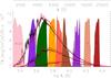 |
Fig. 1 Three sample spectra with solar metallicity, surface gravity log g = 4, and effective temperatures (in decreasing order of flux level) of 6000, 5000, and 4000 K. For each model there are two curves, one corresponding to the Kurucz (1993) models (in black) and one to the more recent spectral energy distributions by Allende Prieto et al. (in prep.; red). Both are shown at a resolving power of R ~ 200 and smoothed (thick lines) to R ~ 8, corresponding to the effective resolution of a broad-band photometric filter. The position and shape of the responses for the different filters under consideration are shown with an arbitrary normalization. The GALEX FUV and the WISE W1 and W2 bandpasses fall outside of the spectral range represented. |
2. Model
As mentioned in the Introduction, this study seeks to quantify in an approximate way the potential for extracting information on a star’s atmospheric parameters from photometry or very-low dispersion spectroscopy. To achieve this goal we use synthetic stellar spectra computed from standard model atmospheres, smooth them with a wide kernel, sample them at the wavelengths of the photometric systems of interest, add noise to them, and finally attempt to recover the atmospheric parameters from the simulated photometry.
We want to explore a wide range in the main atmospheric parameters, keeping the number of variables small enough to be practical. In that spirit, we work with the stellar effective temperature Teff, surface gravity log g1, and the overall abundance of metals relative to hydrogen ([Fe/H]2), ignoring the fact that abundance ratios [X/Fe] may be different from 0 (i.e., non-solar) for some metals X.
Spectral energy distributions (SEDs) sampled fine enough for our purpose are part of the output of standard model atmosphere calculations with the ATLAS9 code (Kurucz 1979, 1993; Castelli & Kurucz 2003; Mészáros et al. 2012). The different versions of ATLAS9 models available over the years correspond to a sequence of improvements regarding input atomic and molecular data, reference abundances, and algorithms. Since in our tests we add noise to the models to simulate observations, and subsequently attempt to recover the atmospheric parameters, it is largely irrelevant which version of the models we adopt. We chose the Kurucz (1993) models over more recent versions since they provide a more complete and regular coverage of late-type stars at very low metallicities, an area of the parameter space of high interest.
Kurucz’s ATLAS9 provides approximate emergent SEDs similar to those internally used in the code to evaluate the energy balance3. They are coarsely sampled, in steps that vary between a few angströms at the UV end (starting at 90 Å) to 20 μm at the IR limit (160 μm). In velocity space the steps are larger in the UV and optical range, at about 4000–9000 km s-1, than in the near- and mid-infrared (1–100 μm), where they range approximately between 1000 and 2000 km s-1).
In addition to this model data set, in some of our tests we use a more recent set of synthetic spectra based on a different batch of ATLAS9 model atmospheres (Mészáros et al. 2012). These are computed with newer line and continuum opacities, different reference zero-point solar abundances, and a different radiative transfer code. The details are not terribly relevant for our purposes, but are described in Allende Prieto et al. (in prep.). The point to stress is that there are important differences between the synthetic SEDs described above and computed by Kurucz (1993) and these newer ones, and this allows us to estimate the impact of systematic errors in the models. Figure 1 illustrates these differences for three models with Teff = 6000, 5000, and 4000 K, in all cases at [Fe/H] = 0 and log g = 4.0.
In some of our experiments we consider the effect of interstellar absorption on the observed spectra. We model reddening following Fitzpatrick (1999; see also Fitzpatrick & Masa 1990, and references therein). We use their software, adopting the average Galactic value for the parameter R ≡ Av/E(B−V) = 3.1.
3. Methodology
Stellar atmospheric parameters can be inferred from observations by adopting a variety of strategies, depending on spectral type and the available data. A recent overview of techniques has been given by Allende Prieto (2016), and further details can be found in Chapters 14–16 of the textbook by Gray (2008). In this paper we are concerned with the information content of a number of important photometric or spectrophotometric systems, and it is therefore appropriate to consider the case in which such (spectro-)photometric measurements are the only data available for the targets of interest.
In order to gain an understanding of the relative impact of random and systematic errors, we consider separately the cases in which only the former or both are included. We also deal with the case where interstellar absorption (reddening) is not present, and study later its impact on the determination of stellar parameters. Even though reddening is always present, there are cases where it may be negligibly small (for stars in the immediate solar neighborhood, at a few parsecs), or where it is accurately known from other measurements, e.g., from IR dust emission maps or diffuse bands observed in spectra towards the same direction).
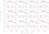 |
Fig. 2 Comparison between the simulated photometric observations (open symbols) and those recovered from the fittings (red asterisks) for a few test cases chosen at random. The labels show the parameters recovered with FERRE (red) and the true values (black). |
We compiled the Kurucz (1993) SED with metallicities between −4.5 and + 0.5 (with 0.5 dex steps), effective temperatures in the range 4000 to 7000 K (250 K steps), and surface gravities spanning between 1.5 and 4.0 (0.5 dex steps). We smoothed the SEDs to mimic the spectral resolution typical of broad-band photometric observations (R ≡ λ/δλ ~ 8; see the smoothed black curves in Fig. 1) or the Gaia spectrophotometers (R ~ 30). We then interpolated in the regular grid of SEDs using cubic Bézier splines to get SEDs for a random set of parameters uniformly distributed over the grid. We finally added random noise to these interpolated fluxes at a level that can be reasonably expected for real observations:
-
10% (0.1 mag) and 7% (0.07 mag) for the GALEX FUV and NUVpassbands, respectively;
-
5% for the SDSS u and z-bands, and 2% for the other SDSS filters;
-
4% for the 2MASS JHKs photometry;
-
4% for the WISE W1 and W2 bandpasses.
In the case of the Gaia BP/RP data, we adopted two values for the signal-to-noise ratio, 50 and 20 (σ = 2% and 5%), independent of wavelength, which are approximately the mean values expected at blue wavelengths for stars with G ≃ 16 and 18 (Bailer-Jones 2010).
The resulting SEDs are analyzed using the optimization code FERRE4 (Allende Prieto et al. 2006), which infers the atmospheric parameters from the very same models used to simulate observations. FERRE couples an optimization algorithm, in this case Powell’s UOBYQA algorithm (Powell 2000), with interpolation in a grid of model spectra. In this analysis we used linear interpolation to avoid adopting exactly the same interpolation scheme used to prepare the simulations.
These tests are ideal in the sense that no systematic errors other than those incurred by adopting linear interpolation in FERRE are considered. However, they are useful to reveal potential degeneracies among the parameters regarding the predicted SEDs. The fact that we have introduced random noise in the simulated fluxes hampers our ability to recover the true underlying model parameters. We examine in particular the effect of including different bandpasses on the recovery of the atmospheric parameters.
4. Photometric tests without reddening
We considered first the simplified situation in which there is no reddening distorting the observed stellar spectra. We studied five combinations of photometric systems, corresponding to the available data:
-
only SDSS ugriz photometry;
-
SDSS and 2MASS JHKs photometry;
-
SDSS, 2MASS, and GALEX FUV and NUV photometry;
-
SDSS, 2MASS, and WISE W1 and W2 photometry;
-
SDSS, 2MASS, GALEX, and WISE photometry.
We ran the simulated data, transformed into normalized logarithmic units, through the fitting code and recovered the parameters for each object. Figure 2 illustrates the input and the output data for one of our experiments with reddening; except for the presence of that parameter, those without reddening are very similar.
For each case we calculate the dispersion between the recovered and the true parameters by finding the width of the distribution excluding 15.85% of the data at each extreme (those with the largest discrepancies) and dividing that value by two. For a Gaussian distribution this value would correspond to 1σ, but this procedure makes the determination robust to a small percentage of outliers. We do this for the full sample of 1000 simulated targets, and only for the roughly 300 that lie at metallicities higher than [Fe/H] = −1. This separation is useful since most stars in the Milky Way reside in the Galactic disk in that metallicity range, and at high metallicities there is significantly more information than at low values owing to the presence of numerous and strong absorption lines in the spectra. In fact, there is nearly no information on metallicity in spectra at [Fe/H] < −3.
Robust standard deviation between the retrieved and true atmospheric parameters for the full sample (−5 ≤ [Fe/H] ≤ + 1) and a metal-rich subsample ([Fe/H] ≥ −1) as a function of the photometric bandpasses included in the numerical experiments.
The results are given in Table 1, and Fig. 3 illustrates the analysis for the full sample in the case when all photometric bandpasses are considered. The uncertainties in all three parameters vary in sync with larger errors for more metal-poor stars, a more modest dependence on effective temperature (in the narrow range where are experiments are contained), and a fairly weak dependence on surface gravity. We find that the average value of the distributions have very small offsets from zero, and therefore the table gives only the robust standard deviation for the distribution of residuals in each parameter. Our statistics are slightly distorted by the fact that solutions cannot be found outside the limits of our model grid, but these distortions appear to be modest.
SDSS photometry (ugriz) alone can constrain fairly well the stellar effective temperature (σ ~ 150 K or about 0.01 dex), but poorly constrains the metallicities or stellar surface gravities. Adding infrared photometry significantly improves the recovery of Teff, but has very little impact on gravity, while the results for [Fe/H] vary depending on the metallicity range: at high metallicity, optical and near-infrared photometry help in recovering this parameter, but offer little leverage for more metal-poor stars. Adding UV photometry can significantly improve the recovery of metallicities and surface gravities for stars at all metallicities.
5. Photometric tests including reddening
In most practical situations interstellar reddening gets in the way, making it more difficult to derive the parameter that has the highest influence on the shape of the spectrum, the effective temperature. Naturally, the determination of the other two atmospheric parameters will be severely affected by the potential confusion between reddening and Teff.
We repeated the experiments described in Sect. 4 adding an additional dimension to the problem, accounting for the effect of reddening as described in Sect. 2. Each of the 1000 simulated observations were reddened for a random value of E(B−V) between 0 and 0.25 mag drawn from a uniform distribution. This range is typical outside a stripe of ±10deg from the Galactic plane.
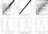 |
Fig. 3 Upper panels: comparison between the parameters recovered with FERRE from our simulations against the true values for the case when all the filters are included. The red curves show a least-squares fit to the data. Bottom panels: histograms of the residuals for each parameter. The red curves correspond to a Gaussian fit to the data, which systematically underestimates the width of the distribution for [Fe/H]; therefore, it is not adopted for the statistics shown in the tables and is discussed in the text. The median offsets of the distributions are 0.03 dex, 6 K, and 0.08 dex for [Fe/H], Teff, and log g, respectively. The straight standard deviations are 0.98 dex, 58 K, and 0.67 dex, while those computed with the robust algorithm described in the text are 0.70 dex, 45 K, and 0.57 dex. |
Similarly to the case in previous section, we used FERRE to recover the atmospheric parameters and the reddening E(B−V) simultaneously (See Fig. 2). The results in this case are summarized in Table 2. Obviously, our ability to recover all the atmospheric parameters is significantly degraded compared to zero-reddening case presented in Sect. 4. Nonetheless, qualitatively, most of our conclusions hold: effective temperatures are already recovered with optical photometry at a level of about 350 K (0.03 dex), and this value improves somewhat adding near-infrared photometry from 2MASS. We now find that our ability to discern the effects of reddening from those of interstellar extinction is substantially improved by folding UV photometry in the data set, and this has a positive impact on all parameters. Finally, adding the mid-IR data from WISE adds very little information.
6. Gaia spectrophotometry
Gaia will provide SEDs for about 109 stars in the Milky Way. Operating in space, it is expected that these data will be very precise, even though the zero-point accuracy will likely be limited by difficulties connecting standard flux laboratory sources and those made with an astronomical instrument (Bohlin et al. 2014).
We repeated the experiments in the previous sections at somewhat higher resolution (R ~ 25), sampling the spectra between 3600 and 10 500 Å with 86 samples evenly distributed in log λ. Such a setup resembles, but is not equal to, the data expected from the Gaia photometers BP/RP. The real data will have a resolving power and sampling rate that varies with wavelength and shows an abrupt discontinuity at about 660 nm where the two overlapping blue (BP) and red (RP) channels meet (see de Bruijne et al. 2014, for more details). In addition, we injected noise at a constant level at all wavelengths (5% and 2%; see Sect. 2), while the actual observations have a signal-to-noise ratio that depends strongly on wavelength (see, e.g., Bailer-Jones 2010). We also assume that the instrumental response is perfectly known (see Jordi 2015 for real BP/RP images and collapsed spectra). Nonetheless, we expect that the impact on our conclusions of simulating the Gaia data in more detail will be modest, especially in comparison with some of our other approximations.
As shown in Table 1, for the Gaia BP/RP spectrophotometry alone, and without extinction in our simulations, we find that we are able to recover the stellar metallicities, effective temperatures, and surface gravities to within 0.2 dex, 23 K, and 0.2 dex, respectively, for a star with G ~ 16 (S/N ~ 50), and within 0.5 dex, 57 K, and 0.4 dex, respectively, at G ~ 18 (S/N ~ 20). Limiting the sample to stars more metal-rich than [Fe/H] = −1, the uncertainty in [Fe/H] improves to 0.1 dex at G ~ 16 and 0.2 dex at G ~ 18. These figures are in fact quite similar to those reported by Bailer-Jones (2010).
As we concluded in the case of photometry, there is increased confusion when reddening is considered (see Table 2). The uncertainties in the recovered values of [Fe/H], Teff, and log g rise to 0.4 dex, 153 K, and 0.3 dex, respectively, for the full sample, or 0.2 dex, 125 K, and 0.3 dex for the subsample at [Fe/H] > −1. In both cases the reddening is recovered with an uncertainty of about 0.03 mag.
7. Systematic errors
It is interesting to explore the impact of systematic errors on the model stellar fluxes. We can get a glimpse of how much such effects can distort our results by analyzing the simulated photometry described above from Kurucz (1993) SEDs with a different set of models from Allende Prieto et al. (in prep.).
The fluxes computed by Allende Prieto et al. (in prep.) are more limited in wavelength coverage (they do not cover in full the GALEX passbands) and parameter space than the Kurucz (1993) SEDs, as described in Sect. 2. For that reason we limit our tests to the optical and infrared filters, and to stars with Teff< 6000 K and [Fe/H] > −1. The limit on Teff is not strict since the new model fluxes are available for Teff> 6000 K, but warmer models are part of a separate bundle from those for cooler temperatures, and including stars between 6000 and 7000 K would significantly complicate the implementation of our tests.
Median offsets and robust standard deviations between the retrieved and true atmospheric parameters for a metal-rich subsample ([Fe/H]≥−1).
The results in this case are shown in Table 3. Unlike Tables 1 and 2, this table includes the median offset between the parameters recovered by FERRE and the true ones in the first three columns in addition to the robust standard deviation in Cols. 4−6, which can be directly compared to those in Table 1 for the case limited to −1 ≤ [Fe/H] ≤ + 1 (although it corresponds to a slightly smaller range in Teff). It should be remembered that the median offsets of the distribution of residuals from zero were negligible when systematic errors were not considered in Sects. 4, 5, and 6.
Overall, the retrieved parameters suffer modest systematic errors compared to the spread even though the differences between the models used in the simulations and the analysis are important (see examples in Fig. 1). The widths of the distributions are very similar to the values reported in Table 1 for [Fe/H] and Teff, but the surface gravity recovered is significantly worse when systematic errors are taken into account.
8. Summary and conclusions
We perform numerical experiments to explore the potential of broad-band photometry and spectrophotometry of stars to infer atmospheric parameters and the interstellar extinction along the line of sight. Our experiments are fairly simplistic in that we ignore systematic errors that result from an imperfect knowledge of the distortions introduced by instruments and, in the case of ground-based observations, the effect of Earth’s atmosphere, but should hold as long as they are significantly smaller than the random uncertainties adopted (2–10%, depending on the instrument and wavelength). As such, our results provide an upper limit to the performance achievable for real data.
We find that photometry over a wide spectral range from the near-UV to the mid-IR can constrain the atmospheric parameters fairly well. While optical data are enough to constrain well the effective temperature of late-type stars, this parameter is retrieved with far better precision by including infrared observations. We show that the determination of surface gravity and metallicity can benefit substantially from the addition of near-UV photometry.
For a similar signal-to-noise ratio, the performance expected for an instrument like the Gaia BP/RP spectrophotometer is better than standard photometric systems with a similar wavelength span. This is not surprising, since both resolution and sampling are much better for BP/RP than for the standard broad-band photometric systems. However, for the faintest stars observed by Gaia, photon noise will limit significantly the atmospheric parameters determined from the BP/RP observations.
Photometric searches for ultra-metal-poor stars can benefit enormously from counting on UV passbands. In our tests without reddening, the success rate at [Fe/H] ≤ −3, defined as the fraction of stars correctly identified in that range, and the false-positive rate are 59% and 42%, respectively, using only SDSS photometry, but these figures change to 79% and 22%, respectively, when the GALEX filters are included in the observations.
The effect of interstellar absorption on the observations hampers our ability to recover the stellar atmospheric parameters. Only with wide wavelength coverage – in particular in the blue and into the near-UV – and high signal-to-noise ratios can reddening be cleanly disentangled from variations in the atmospheric parameters.
It will be very interesting to verify our expectations with real data, although it goes beyond the scope of the present paper and will likely require some sort of zero-point calibration of the synthetic photometry. In addition, in our numerical experiments we have sampled the SEDs at specific wavelengths corresponding to each of the bandpasses under study, but for practical applications it is necessary to convolve the model SEDs with the filter responses since a filter’s effective wavelength depends on the stellar spectrum.
Our main conclusion is that wide-area photometry at multiple wavelengths is a promising path for characterizing the stellar populations of the Milky Way and other nearby galaxies where stars can be resolved. Following up on pioneering studies (e.g., Ivezić et al. 2008), projects that already do this in a homogeneous fashion such as ALHAMBRA (Moles et al. 2008), J-PLUS and JPAS (Benítez et al. 2014), PAU (Castander et al. 2012), or the Gaia mission will demonstrate the potential and the limitations of this technique.
Here g is the gravitational acceleration at the surface of the star in units of cm s-2; therefore, g = GM/R2, where G is the gravitational constant, M is the stellar mass, and R is the stellar radius.
We use the standard notation ![Mathematical equation: \hbox{${\rm [X/Y]}= \log \frac{\rm N(X)}{\rm N(Y)} - \log \left( \frac{\rm N(X)}{\rm N(Y)}\right)_{\odot}$}](/articles/aa/full_html/2016/11/aa28789-16/aa28789-16-eq72.png) , where N(X) represents the number density of nuclei of the element X.
, where N(X) represents the number density of nuclei of the element X.
Accessible from http://kurucz.harvard.edu
FERRE is available from http://hebe.as.utexas.edu/ferre
Acknowledgments
I am grateful to David S. Aguado y Jonay González Hernández for valuable discussions and constructive criticism on this manuscript. I also appreciate useful suggestions from the referee, Eduard Masana, and the excellent work by Helenka Kinnan improving the language. My research has been generously supported by the Spanish MINECO (AYA2014-56359-P).
References
- Allen de Prieto, C. 2016, Liv. Rev. Sol. Phys., 13, 1 [CrossRef] [Google Scholar]
- Allen de Prieto, C., Beers, T. C., Wilhelm, R., et al. 2006, ApJ, 636, 804 [NASA ADS] [CrossRef] [Google Scholar]
- Aparicio Villegas, T., Alfaro, E. J., Cabrera-Caño, J., et al. 2010, AJ, 139, 1242 [NASA ADS] [CrossRef] [Google Scholar]
- Bailer-Jones, C. A. L. 2004, A&A, 419, 385 [NASA ADS] [CrossRef] [EDP Sciences] [Google Scholar]
- Bailer-Jones, C. A. L. 2010, MNRAS, 403, 96 [NASA ADS] [CrossRef] [Google Scholar]
- Bailer-Jones, C. A. L., Andrae, R., Arcay, B., et al. 2013, A&A, 559, A74 [NASA ADS] [CrossRef] [EDP Sciences] [Google Scholar]
- Benitez, N., Dupke, R., Moles, M., et al. 2014, Arxiv e-prints [arXiv:1403.5237] [Google Scholar]
- Bessell, M. S. 2005, ARA&A, 43, 293 [NASA ADS] [CrossRef] [Google Scholar]
- Bohlin, R. C., Gordon, K. D., & Tremblay, P.-E. 2014, PASP, 126, 711 [NASA ADS] [Google Scholar]
- de Bruijne, J. H. J. 2012, Ap&SS, 341, 31 [NASA ADS] [CrossRef] [Google Scholar]
- de Bruijne, J. H. J., Rygl, K. L. J., & Antoja, T. 2014, EAS Pub Ser., 67, 23 [CrossRef] [EDP Sciences] [Google Scholar]
- Castander, F. J., Ballester, O., Bauer, A., et al. 2012, Proc. SPIE, 8446, 84466D [CrossRef] [Google Scholar]
- Castelli, F., & Kurucz, R. L. 2003, Modelling of Stellar Atmospheres, 210, A20 [Google Scholar]
- Fitzpatrick, E. L. 1999, PASP, 111, 63 [NASA ADS] [CrossRef] [Google Scholar]
- Fitzpatrick, E. L., & Massa, D. 1990, ApJS, 72, 163 [NASA ADS] [CrossRef] [Google Scholar]
- Fukugita, M., Ichikawa, T., Gunn, J. E., et al. 1996, AJ, 111, 1748 [NASA ADS] [CrossRef] [Google Scholar]
- Gray, D. F. 2008, The Observation and Analysis of Stellar Photospheres (Cambridge, UK: Cambridge University Press) [Google Scholar]
- Jordi, C. 2015, Highlights of Spanish Astrophysics VIII, 390 [Google Scholar]
- Jordi, C., Gebran, M., Carrasco, J. M., et al. 2010, A&A, 523, A48 [NASA ADS] [CrossRef] [EDP Sciences] [Google Scholar]
- Ivezić, Ž., Sesar, B., Jurić, M., et al. 2008, ApJ, 684, 287 [NASA ADS] [CrossRef] [Google Scholar]
- Kurucz, R. 1993, ATLAS9 Stellar Atmosphere Programs and 2 km s-1 grid, Kurucz CD-ROM No. 13 (Cambridge, Mass.: Smithsonian Astrophysical Observatory), 13 [Google Scholar]
- Kurucz, R. L. 1979, ApJS, 40, 1 [NASA ADS] [CrossRef] [Google Scholar]
- Lenz, D. D., Newberg, J., Rosner, R., Richards, G. T., & Stoughton, C. 1998, ApJS, 119, 121 [NASA ADS] [CrossRef] [MathSciNet] [Google Scholar]
- Martin, D. C., Fanson, J., Schiminovich, D., et al. 2005, ApJ, 619, L1 [Google Scholar]
- Masana, E., Jordi, C., & Ribas, I. 2006, A&A, 450, 735 [NASA ADS] [CrossRef] [EDP Sciences] [Google Scholar]
- Mészáros, S., Allen de Prieto, C., Edvardsson, B., et al. 2012, AJ, 144, 120 [NASA ADS] [CrossRef] [Google Scholar]
- Powell, M. J. D. 2000, UOBYQA: unconstrained optimization by quadratic approximation, report DAMTP 2000/NA14 (University of Cambridge) [Google Scholar]
- Skrutskie, M. F., Cutri, R. M., Stiening, R., et al. 2006, AJ, 131, 1163 [NASA ADS] [CrossRef] [Google Scholar]
- Wright, E. L., Eisenhardt, P. R. M., Mainzer, A. K., et al. 2010, AJ, 140, 1868 [NASA ADS] [CrossRef] [Google Scholar]
All Tables
Robust standard deviation between the retrieved and true atmospheric parameters for the full sample (−5 ≤ [Fe/H] ≤ + 1) and a metal-rich subsample ([Fe/H] ≥ −1) as a function of the photometric bandpasses included in the numerical experiments.
Median offsets and robust standard deviations between the retrieved and true atmospheric parameters for a metal-rich subsample ([Fe/H]≥−1).
All Figures
|
Fig. 1 Three sample spectra with solar metallicity, surface gravity log g = 4, and effective temperatures (in decreasing order of flux level) of 6000, 5000, and 4000 K. For each model there are two curves, one corresponding to the Kurucz (1993) models (in black) and one to the more recent spectral energy distributions by Allende Prieto et al. (in prep.; red). Both are shown at a resolving power of R ~ 200 and smoothed (thick lines) to R ~ 8, corresponding to the effective resolution of a broad-band photometric filter. The position and shape of the responses for the different filters under consideration are shown with an arbitrary normalization. The GALEX FUV and the WISE W1 and W2 bandpasses fall outside of the spectral range represented. |
| In the text | |
|
Fig. 2 Comparison between the simulated photometric observations (open symbols) and those recovered from the fittings (red asterisks) for a few test cases chosen at random. The labels show the parameters recovered with FERRE (red) and the true values (black). |
| In the text | |
|
Fig. 3 Upper panels: comparison between the parameters recovered with FERRE from our simulations against the true values for the case when all the filters are included. The red curves show a least-squares fit to the data. Bottom panels: histograms of the residuals for each parameter. The red curves correspond to a Gaussian fit to the data, which systematically underestimates the width of the distribution for [Fe/H]; therefore, it is not adopted for the statistics shown in the tables and is discussed in the text. The median offsets of the distributions are 0.03 dex, 6 K, and 0.08 dex for [Fe/H], Teff, and log g, respectively. The straight standard deviations are 0.98 dex, 58 K, and 0.67 dex, while those computed with the robust algorithm described in the text are 0.70 dex, 45 K, and 0.57 dex. |
| In the text | |
Current usage metrics show cumulative count of Article Views (full-text article views including HTML views, PDF and ePub downloads, according to the available data) and Abstracts Views on Vision4Press platform.
Data correspond to usage on the plateform after 2015. The current usage metrics is available 48-96 hours after online publication and is updated daily on week days.
Initial download of the metrics may take a while.