| Issue |
A&A
Volume 595, November 2016
|
|
|---|---|---|
| Article Number | A44 | |
| Number of page(s) | 6 | |
| Section | Interstellar and circumstellar matter | |
| DOI | https://doi.org/10.1051/0004-6361/201527721 | |
| Published online | 26 October 2016 | |
A near-infrared interferometric survey of debris-disc stars
V. PIONIER search for variability⋆
1 European Southern Observatory,
Alonso de Cordova 3107, Vitacura,
Casilla 19001, Santiago
19, Chile
2 Steward Observatory, Department of
Astronomy, University of Arizona, 993 N. Cherry Ave, Tucson, AZ
85721,
USA
e-mail: This email address is being protected from spambots. You need JavaScript enabled to view it.
3 Space sciences, Technologies and
Astrophysics Research (STAR) Institute, Université de Liège,
19c Allée du Six
Août, 4000
Liège,
Belgium
4 Univ. Grenoble Alpes, IPAG,
38000
Grenoble,
France
5 CNRS, IPAG, 38000
Grenoble,
France
6 European Southern Observatory,
Karl-Schwarzschild-Straße
2, 85748
Garching,
Germany
7 Observatoire de Genève, Université de
Genève, 51 ch. des
Maillettes, 1290
Versoix,
Switzerland
8 Institute of Astronomy, University of
Cambridge, Madingley
Road, CB3 0HA,
UK
9 Infrared Processing and Analysis
Center, California Institute of Technology, Pasadena, CA
91125,
USA
10 NASA Exoplanet Science Institute,
California Institute of Technology, 770 S. Wilson Ave., Pasadena, CA
91125,
USA
11 Instituto de Física y Astronomía,
Facultad de Ciencias, Universidad de Valparaíso, Av. Gran Bretaña 1111, Playa Ancha,
Valparaíso,
Chile
Received:
10
November
2015
Accepted:
14
August
2016
Abstract
Context. Extended circumstellar emission has been detected within a few 100 milli-arcsec around ≳10% of nearby main sequence stars using near-infrared interferometry. Follow-up observations using other techniques, should they yield similar results or non-detections, can provide strong constraints on the origin of the emission. They can also reveal the variability of the phenomenon.
Aims. We aim to demonstrate the persistence of the phenomenon over the timescale of a few years and to search for variability of our previously detected excesses.
Methods. Using Very Large Telescope Interferometer (VLTI)/Precision Integrated Optics Near Infrared ExpeRiment (PIONIER) in H band we have carried out multi-epoch observations of the stars for which a near-infrared excess was previously detected using the same observation technique and instrument. The detection rates and distribution of the excesses from our original survey and the follow-up observations are compared statistically. A search for variability of the excesses in our time series is carried out based on the level of the broadband excesses.
Results. In 12 of 16 follow-up observations, an excess is re-detected with a significance of > 2σ, and in 7 of 16 follow-up observations significant excess (> 3σ) is re-detected. We statistically demonstrate with very high confidence that the phenomenon persists for the majority of the systems. We also present the first detection of potential variability in two sources.
Conclusions. We conclude that the phenomenon responsible for the excesses persists over the timescale of a few years for the majority of the systems. However, we also find that variability intrinsic to a target can cause it to have no significant excess at the time of a specific observation.
Key words: techniques: interferometric / circumstellar matter / planetary systems / zodiacal dust
Based on observations made with ESO Telescopes at the La Silla Paranal Observatory under program IDs 088.C-0266, 089.C-0365, 090.C-0526, 091.C-0576, 091.C-0597, 094.C-0232, and commissioning data.
F.R.S.-FNRS Research Associate.
© ESO, 2016
1. Introduction
The detection of circumstellar near-infrared (near-IR) excess emission at the level of ~1% within a few 100 milli-arcsec (mas) around nearby, mature main-sequence stars, remains enigmatic. It is generally attributed to the presence of hot circumstellar dust. The detections have been made using near-IR interferometry mostly employing the instruments Fiber Linked Unit for Optical Recombination (FLUOR) at the Center for High Angular Resolution Astronomy (CHARA) array (e.g., Absil et al. 2006, 2013) and Precision Integrated Optics Near Infrared ExpeRiment (PIONIER) at the Very Large Telescope Interferometer (VLTI; Defrère et al. 2012; Ertel et al. 2014). These very accurate instruments are pushed to their limits by such observations in terms of both statistical accuracy and ability to calibrate the data obtained. Until now, only two detections could be confirmed from repeated observations: Vega (Absil et al. 2006; Defrère et al. 2011) and β Pic (Defrère et al. 2012; Ertel et al. 2014).
Mid-infrared (mid-IR) nulling observations reveal no correlation between near-IR and mid-IR excesses (Mennesson et al. 2014) and follow-up observations of the near-IR excess stars, attempting to detect polarized scattered light emission from the circumstellar dust, did not result in significant detections (Marshall et al. 2016). When combined with the near-IR detections, these data provide strong and valuable constraints – even in the case of upper limits – on the emission at different wavelengths and on different spatial scales, and thus on the origin of the excesses (Lebreton et al. 2013). However, variability of the excesses needs to be characterized or ruled out. In the case of non-detections in follow-up observations, the original detections need to be confirmed and it needs to be established that the excesses persist from the original detections to the follow-up observations. At the same time, the detection and analysis of variability can inform us regarding the origin of the emission. Theoretical models face severe problems in explaining the large amounts of dust in the innermost regions of these systems, needed to produce the excess (Bonsor et al. 2012, 2013, 2014). The short orbital period and high surface density are thought to result in rapid removal of the dust from the systems by the stellar radiation pressure (Backman & Paresce 1993). The detection or not of variability can enable us to distinguish between continuous, episodic, and catastrophic dust production.
In this paper, we present new data obtained using VLTI/PIONIER. Several repeat observations were made of the stars for which an excess had previously been detected with this instrument and observation technique (Ertel et al. 2014), with the intention of demonstrating the persistence of the phenomenon over time and to search for variability. We summarize our observation strategy and data processing in Sect. 2. In Sect. 3 we present our analysis of the detections and non detections. We statistically show that the detection rate for our follow-up observations of known excess stars is significantly higher than for our original survey of stars without previous information on the presence or absence of near-IR excess. In Sect. 3.2 we present a search for variability in the broadband excesses of single objects and report on the first detection of potential variability in two of our targets. In Sect. 4 we discuss possible statistical and systematic effects and argue that they are very unlikely to produce this result. We present our conclusions in Sect. 5.
2. Data acquisition and processing
2.1. Observations
We re-observed in H band several times six of the nine stars with nominal detections and one of the three stars with tentative detections from our original PIONIER survey (Ertel et al. 2014). We focus here on this clean sample of stars with excesses detected using the same instrument and technique and in the same band (H band) as we employ for our follow-up observations. Only for these targets can we confidently expect a re-detection and directly compare our detection statistics from our original PIONIER survey with our follow-up observations. The new data presented in this work were obtained in August 2013 and October 2014. In addition, we consider data of HD 172555 obtained in April 2014 in the context of a dedicated study. We compare our detection rate and excess levels from the new observations with our original survey (Ertel et al. 2014) and previous observations of β Pic (HD 39060, Defrère et al. 2012). The targets and the observing dates are listed in Table 1.
Observing log, excesses, and variability.
For our observations, we followed closely the strategy motivated and outlined in Ertel et al. (2014), which we only briefly summarize here. All observations were carried out in H band using the PIONIER beam combiner on the VLTI in combination with the 1.8 m Auxiliary Telescopes in the compact configuration (baselines between 11 m and 36 m). We simultaneously obtained squared visibility measurements on six baselines and closure phase measurements on four telescope triplets with each science observation. A sequence of three observations on a science target was taken, bracketed and interleaved by observations of calibrators (CAL-SCI-CAL-SCI-CAL-SCI-CAL). At least three different calibrators were selected for each sequence and each science observation was bracketed by two different calibrators. The calibrators were selected from the catalog of Mérand et al. (2005). Observations were carried out in SMALL spectral resolution (three channels across the H band). The FOWLER read-out mode and the fast AC mode were used and the number of steps read in one scan (NREAD) was set to 1024 with a scan length of 60 μm.
The observing conditions were in general well suited for our observations (seeing and coherence time <1.5′′ and >2 ms, respectively, thin clouds at most). Only on one night, 9-Aug.-2013, were the conditions highly variable with occasionally very large seeing values (>2′′) and short coherence time (~1 ms). A detailed discussion of the systematic effects produced by such observing conditions is presented in Appendix A. We discard all data taken during this night from our statistical analysis, because they have to be considered unreliable as discussed in the appendix.
2.2. Data reduction, calibration, and excess measurement
We reduce our new data using the standard PIONIER pipeline version 3.30 (Le Bouquin et al. 2011). As for our observing strategy, for the calibration and excess measurements we closely followed the procedure motivated and outlined by Ertel et al. (2014). First, a global calibration of each night was performed to correct for the effect of field rotation on the instrumental visibilities (due to polarization effects in the VLTI optical train; Le Bouquin et al. 2012; Ertel et al. 2014). Then, we selected pairs of a science observation and the preceding or following calibrator observation without using the same calibrator observation to calibrate two science observations. We also avoided using different observations of the same calibrator for the calibration of different observations of one science target. Calibrator observations with large noise, systematically low squared visibilities in most baselines compared to the other calibrators (indicative of a companion or extended circumstellar emission that might be caused, for example, by stellar mass loss on the post-main sequence) or with signs of closure phase signal (indicative of a companion) were excluded. Both render a calibrator unusable. Finally, we fit our simple exozodiacal dust model (a homogeneous emission filling the entire field of view) to all squared visibility data obtained in one observing sequence of a target to measure the flux ratio fCSE between circumstellar emission and star (disk-to-star flux ratio) and its uncertainty σf. Ertel et al. (2014) contains details of the procedure and the stellar photometry and parameters used.
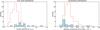 |
Fig. 1 Excess distribution (left) and distribution of uncertainties on the disk-to-star flux ratio (right). The blue histogram represents our H band follow-up observations of previous H band detections with PIONIER. The red line shows the distribution for our original survey (Ertel et al. 2014). Vertical dashed lines are plotted at fCSE/σf = −3 and fCSE/σf = + 3 for the excess distribution and at the median uncertainty (1.6 × 10⁻³) of our follow-up observations for the uncertainty distribution. |
The survey data were originally reduced using the PIONIER pipeline version 2.51. We re-reduced and calibrated these data using the pipeline version 3.30 and found consistent results. In order to avoid having different (but fully consistent) numbers in the literature for these observations, results from Ertel et al. (2014) were used. The data obtained for β Pic before 2012 have been published by Defrère et al. (2012). These observations do not follow our optimized observing strategy, but significantly more data have been taken during each run (typically half a night dedicated to one target). The calibration and analysis performed in Defrère et al. (2012) has been optimized for these data. Since we do not see any reason to update these procedures, and in order to avoid having different (but fully consistent) numbers in the literature, we have re-used these results.
3. Results
3.1. Persistence of the excesses
In order to demonstrate the persistence of our detections, we would ideally like to re-detect every excess in each observation. However, this is unrealistic, since most of our detections are close to our sensitivity limits. Such an excess may be measured to be above the threshold in one observation but below it in another one with the same sensitivity due to statistical errors. Thus, a non-detection of significant excess does not necessarily imply that the excess is no longer present. In fact, we only re-detect the excesses in ~50% of our follow-up observations at a significance >3σ. In our original survey of 92 stars (out of which 85 were used to derive clean statistics), we found an excess detection rate of 10.6+ 4.3-2.5%. We find a mean of the excess significance of χCSE = fCSE/σf of  from our original survey and of
  from our follow-up observations.
To test if the difference in  between the two samples is statistically significant, we use a two sample Anderson-Darling (AD) test (Scholz & Stephens 1987) to see if the distribution of χCSE from our original survey and that from our follow-up observations (including multiple observations of a target) are statistically consistent. If they were found to be consistent, this would indicate that differences in χCSE are simply caused by statistical fluctuations in our data. Furthermore, this would suggest that our detections are caused by imperfectly understood statistical errors that are not repeatable for a given observation but cause false detections with the same probability in repeated observations. If χCSE is found to be significantly higher among the stars observed during our follow-up campaigns, this would mean that an excess is indeed present and persistent over time for at least the majority of our detections.
For almost all targets the original detection was made during our original survey. Only for β Pic was the first detection made during two nights in December 2010 and one night in November 2011. Defrère et al. (2012) combined all these data to measure the excess with the best accuracy (no significant variability was found), but the excess was nominally detected in all data sets. Here, we consider the detection over the two nights in December 2010 as the original detection and each later observation (including the observations in November 2011 and from our original survey) as follow-up observations.
The distribution of χCSE for our original survey and our follow-up observations is shown in Fig. 1 (left panel). The AD test yields a probability of only 5.7 × 10⁻⁵ that these two samples are drawn from the same distribution, which allows us to reject this hypothesis. The right panel of Fig. 1 shows the distribution of σf, illustrating that the sensitivity of our follow-up observations (mean  , median
  ) is similar to that of our original survey (
 ,
,  ).
).
The excess around β Pic is our clearest detection but has been hypothesized to originate from forward scattering in the outer, edge-on seen disk (Defrère et al. 2012). To test the impact of this potential false positive, we repeated the AD test excluding this star and still find a probability of only 2.2 × 10⁻³ that the two samples are drawn from the same distribution. β Pic with its massive, young, edge-on seen debris disk is the only plausible candidate for such a false detection, and even for this star Defrère et al. (2012) rule out that more than 50% of the excess can be produced by forward scattering in the outer disk. We thus reject with very high confidence our null hypothesis that the distributions of χCSE from our survey and follow-up observations are drawn from the same distribution. We thus conclude that an excess was still present and persistent around the majority of our targets during follow-up observations.
3.2. Variability in single targets
We have demonstrated that for a significant fraction of our targets the excess persists over the timescale of a few years. However, our analysis does not allow us to characterize or rule out variability of single sources. In the following, we present a search for variability of the detected excesses. We focus on the broadband excesses (integrated over the three spectral channels), where variability is most readily detectable due to the higher significance of the detections compared to the spectrally dispersed data. A more sophisticated search for variability including the spectral slope of the emission requires detailed modeling of the systems and depends on model assumptions. We defer this analysis together with the production of sensitive upper limits on targets without detected variability and a theoretical interpretation of the results to a forthcoming, dedicated paper.
Our time series of the excess measurements are plotted in Fig. 2. We check whether the single excess measurements for a target deviate significantly from their error weighted mean. The significance ΔCSE of this deviation is computed as 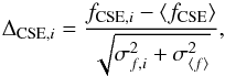 (1)where fCSE,i and σf,i are the flux ratio from a single measurement and its error, ⟨fCSE⟩ is the error weighted mean of all measurements of one target, and
  is the standard deviation of this mean. We again discard from our analysis the data excluded in Sect. 3.1. A significant deviation (>3σ) is found for one target, HD 7788 (Table 1).
We emphasize that this is a simple but conservative metric. It requires, however, that all errors are well understood (see discussion in Sect. 4). A statistical test of the distribution of the excess measurements for a given target against a normal distribution would be a more sensitive tracer of variability, but is not yet possible due to the limited number of points available for each target. We note that for HD 210302 the measurements from the nights of 24-Jul.-2012 and 10-Aug.-2013 deviate from each other by 3.5 times their respective error bars added in quadrature. The first measurement shows significant excess (3.3σ) while the latter one and the one obtained on 11-Oct.-2014 are consistent with no excess. This may thus be considered as a tentative indication that the excess has dropped below our sensitivity between July 2012 and August 2013. However, the largest ΔCSE we find for this star is only 2.77 and we thus consider this variation not significant. For all other targets, the broadband excess measurements are consistent with constant excess over the period they were monitored.
We conclude that with HD 7788 we found the first strong candidate for significant variability of the faint near-IR excess around a nearby main sequence star. As can be seen in Fig. 2, the excess disappears (given our sensitivity) from the first detection to the second observation about one year later and is re-detected approximately one year after that.
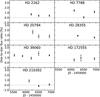 |
Fig. 2 Time series of the excesses. |
4. Discussion
The results from the AD test show that the detection rate from our follow-up observations of stars with previously detected excesses is significantly higher than from our original survey of stars without previous information on the presence of near-IR excesses. We concluded in Sect. 3.1 that this is evidence for a persistence of the excesses around the majority of our targets over timescales of several months to a few years. This conclusion, based on the statistics from our whole samples, is only valid if repeated false detections around specific targets can be ruled out as a cause for the higher detection rate. If the statistical errors are well understood, they will not produce a significant number of false detections. If they were underestimated, they had been expected to produce false detections with the same probability as in any of our observations. They had not been reproducible for a given target during different observation nights. Thus, effects that fall into this category, such as an underestimation of the piston noise in our data, can be ruled out as a cause of the higher detection rate in our follow-up observations based on the AD test results. Other errors that are not reproducible from one observation to another (at a random night, time of the night, and observation condition), such as the presence of an unknown effect of seeing, coherence time, or pointing direction of the observations, or the quality of the alignment of the instrument for the observing night can be ruled out based on the same arguments.
Any systematic effects common to most observations of our excess targets remain to be excluded. Such effects could be related to the science target itself or the calibrators used (underestimation or overestimation of the stellar diameter of the science target or calibrator, respectively). Systematics related to specific calibrators can result in repeatable errors, since the same calibrators (the best ones available) were used for most of the observations of a given science target. Calibrators with faint companions or extended circumstellar emission (bad calibrators) would however only reduce the detected excesses and would not cause false detections.
The targets for which excess has been detected, and associated calibrators, are not particularly bright or have large diameters compared to our whole survey sample. Global systematics in estimating the diameters of both science targets and calibrators would result in a global shift in the distribution of χCSE toward positive or negative excesses, which is not seen in our survey statistics. Furthermore, uncertainties on stellar diameters are minimized by observing at short baselines, where both science targets and calibrators are marginally resolved at most and the remaining uncertainties are well considered in our excess and error estimation. In Table 1, we list the flux ratio derived from all data taken in one observing sequence on a target together with its uncertainty separated in statistical and systematic errors. The flux ratio fCSE is related to the ratio  between measured and predicted squared visibility following
 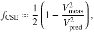 (2)(di Folco et al. 2007). Statistical errors are estimated from the scatter of the single measurements in one observation sequence on a science target using bootstrapping (Defrère et al. 2012; Ertel et al. 2014). They represent the combined uncertainties on measuring the raw visibilities due to piston and photon noise and due to apparent noise in the transfer function attributed to the potential presence of bad calibrators in our data (Mérand et al., in prep.; Ertel et al., in prep.). The systematic uncertainties represent the contribution from uncertain diameters of our science targets and calibrators and a minor contribution from the chromaticism of the instrument (Ertel et al. 2014). For HD 20794 the uncertainties on the photometry used to estimate the stellar diameter from surface brightness relations result in a large uncertainty on the stellar diameter. For all other stars we find the statistical uncertainties dominate the systematic ones. We thus consider any of the discussed effects to be very unlikely to cause false detections in our data.
Above, we have argued that statistical or systematic errors are very unlikely to explain the repeated detection of excess around our science targets. This discussion, however, does not rule out that systematic errors related, for example, to pointing direction, elevation, or instrument alignment (observation night) can produce spurious variability in the signal detected. This could lead to a false detection of variability in the case of HD 7788. In Ertel et al. (2014), we showed that the distribution of excess significance for the non-detections in our original survey is well behaved, following a Gaussian distribution with a standard deviation close to one. This suggests that errors affecting a single point (the visibility obtained on a single baseline or on all baselines during one observation of a science target) are well estimated by (i) our strategy to execute three consecutive observations of a science target and to include the scatter of all 18 points (six baselines for each of three observations) in our error estimates and (ii) the degree of partial correlation of the data considered in our error estimates (Ertel et al. 2014). It also suggests that potential errors affecting the whole observation sequence of a science target such as elevation, time dependence, or magnitude dependence are well calibrated out by our strategy of using three to four different calibrators surrounding our science target within typically 10° and having very similar magnitudes to our science targets. Situations where these effects produce a false detection can therefore be considered as very unlikely. Unfortunately, based on this statistical argument we cannot rule out completely that such an error is present and responsible for the measured variability of HD 7788. We thus consider HD 7788 as the first strong candidate of significant variability, but emphasize that more data in the form of denser and longer time series are needed to confirm this result. In addition, we consider the tentative measurement of variability around HD 210302 another potential candidate. In both cases the u-v-coverage during all observations is similar, thus we consider a different u-v-coverage in combination with a specific excess geometry (e.g., an edge-on disk) very unlikely to be the cause of the excess variations measured.
Although our intention here is to demonstrate the persistence of the excesses, but not to discuss their nature, we note that it has been demonstrated by Marion et al. (2014) that the availability of closure phase data from PIONIER observations enables us to distinguish between the presence of a point-like companion and extended emission as a cause for the signal.
5. Summary and conclusions
We have demonstrated that the phenomenon causing the near-infrared excess around nearby main sequence stars persists over timescales of a few years for the majority of our detections. We have also detected with HD 7788 the first strong candidate of significant excess variability with HD 210302 being another tentative candidate. In the case of HD 7788, the excess seems to disappear (given our sensitivity limits) within one year, but is re-detected one year after that, while in the case of HD 210302 the excess seems to have faded away after the initial detection. We conclude that an excess can be expected to be present around most of our targets during past follow-up observations. Such observations to characterize detected excesses are generally not hindered by strong variability on timescales of several months to a few years. However, the potential variability in two sources demonstrates that a single star cannot be expected to show significant excess at a given observation. Thus, we conclude that for any given case a small sample of stars needs to be observed in order to guarantee the success of a follow-up observation.
Available at http://www.jmmc.fr/aspro
Available at http://www.jmmc.fr/searchcal
Available at http://cdsweb.u-strasbg.fr/
Acknowledgments
This work has significantly benefited from the discussion at the hot dust workshop (JPL/CalTech, May 2015) organized by B. Mennesson and R. Millan-Gabet. S. Ertel, J.-C. Augereau, and A. Bonsor thank the French National Research Agency (ANR, contract ANR-2010 BLAN-0505-01, EXOZODI) and PNP-CNES for financial support. J. Olofsson acknowledges support from the ALMA/Conicyt Project 31130027. PIONIER is funded by the Université Joseph Fourier (UJF), the Institut de Planétologie et d’Astrophysique de Grenoble (IPAG), the Agence Nationale pour la Recherche (ANR-06-BLAN-0421 and ANR-10-BLAN-0505), and the Institut National des Science de l’Univers (INSU PNP and PNPS). The integrated optics beam combiner is the result of a collaboration between IPAG and CEA-LETI based on CNES R&T funding. This research has made use of the Jean-Marie Mariotti Center Aspro1 and SearchCal2 services, the latter co-developped by FIZEAU and LAOG/IPAG, and of the CDS Astronomical Databases SIMBAD and VIZIER3. The authors warmly thank everyone involved in the VLTI project.
References
- Absil, O., di Folco, E., Mérand, A., et al. 2006, A&A, 452, 237 [NASA ADS] [CrossRef] [EDP Sciences] [Google Scholar]
- Absil, O., Defrère, D., Coudé du Foresto, V., et al. 2013, A&A, 555, A104 [NASA ADS] [CrossRef] [EDP Sciences] [Google Scholar]
- Backman, D. E., & Paresce, F. 1993, in Protostars and Planets III, eds. E. H. Levy, & J. I. Lunine, 1253 [Google Scholar]
- Bonsor, A., Augereau, J.-C., & Thébault, P. 2012, A&A, 548, A104 [NASA ADS] [CrossRef] [EDP Sciences] [Google Scholar]
- Bonsor, A., Raymond, S. N., & Augereau, J.-C. 2013, MNRAS, 433, 2938 [NASA ADS] [CrossRef] [Google Scholar]
- Bonsor, A., Raymond, S. N., Augereau, J.-C., & Ormel, C. W. 2014, MNRAS, 441, 2380 [NASA ADS] [CrossRef] [Google Scholar]
- Defrère, D., Absil, O., Augereau, J.-C., et al. 2011, A&A, 534, A5 [NASA ADS] [CrossRef] [EDP Sciences] [Google Scholar]
- Defrère, D., Lebreton, J., Le Bouquin, J.-B., et al. 2012, A&A, 546, L9 [NASA ADS] [CrossRef] [EDP Sciences] [Google Scholar]
- di Folco, E., Absil, O., Augereau, J.-C., et al. 2007, A&A, 475, 243 [NASA ADS] [CrossRef] [EDP Sciences] [Google Scholar]
- Ertel, S., Absil, O., Defrère, D., et al. 2014, A&A, 570, A128 [NASA ADS] [CrossRef] [EDP Sciences] [Google Scholar]
- Le Bouquin, J.-B., Berger, J.-P., Lazareff, B., et al. 2011, A&A, 535, A67 [NASA ADS] [CrossRef] [EDP Sciences] [Google Scholar]
- Le Bouquin, J.-B., Berger, J.-P., Zins, G., et al. 2012, in Proc SPIE, 8445 [Google Scholar]
- Lebreton, J., van Lieshout, R., Augereau, J.-C., et al. 2013, A&A, 555, A146 [NASA ADS] [CrossRef] [EDP Sciences] [Google Scholar]
- Marion, L., Absil, O., Ertel, S., et al. 2014, A&A, 570, A127 [NASA ADS] [CrossRef] [EDP Sciences] [Google Scholar]
- Marshall, J. P., Cotton, D. V., Bott, K., et al. 2016, ApJ, 825, 124 [NASA ADS] [CrossRef] [Google Scholar]
- Mennesson, B., Millan-Gabet, R., Serabyn, E., et al. 2014, ApJ, 797, 119 [NASA ADS] [CrossRef] [Google Scholar]
- Mérand, A., Bordé, P., & Coudé du Foresto, V. 2005, A&A, 433, 1155 [NASA ADS] [CrossRef] [EDP Sciences] [Google Scholar]
- Scholz, F. W., & Stephens, M. A. 1987, J. Am. Stat. Assoc., 82, 918 [Google Scholar]
Appendix A: Effects of short and variable coherence time
The stability of PIONIER observations is generally very high, even in mediocre observation conditions. There are, however, limits to this caused by technical limitations of the instrument. We mentioned in Sect. 2.1 that in one night, 9-Aug.-2013, the observation conditions were highly variable with occasionally very large seeing values (>2′′) and short coherence time (~1 ms). Since we aim for very high statistical and calibration accuracy in our data, such conditions are problematic and we discuss the consequences here.
The fringe contrast and thus the visibility is measured with PIONIER by scanning the optical path delay (OPD) and recording the resulting contrast over time (i.e., over OPD). This is done
with very high speed (in our case, the integration time of a single point of the scan is ~1 ms with one scan being sampled by 1024 points) in order to freeze the effects of atmospheric turbulence. As long as the turbulence is slow enough (long enough coherence time), this produces a very stable transfer function (TF, i.e., the contrast reached on a point source considering all instrumental and atmospheric effects). Our experience has shown that this is the case as long as the coherence time is longer than ~2 ms. If the coherence time drops significantly below this value, the TF drops. This can be understood as a loss of temporal coherence of the star light due to atmospheric turbulence that can no longer be compensated by scanning the fringes even faster because of instrumental limitations in both scan speed and limiting magnitude.
In the night of 9-Aug.-2013, the coherence time was variable over the course of the night, ranging from 2 ms to below 1 ms. For some observing sequences the coherence time was still at an acceptable level. This means they can, in principle, be calibrated well. The uncertainty from this calibration as well as the statistical uncertainty estimated from the scatter of the contrast measured on single scans are comparable to those for data obtained in more stable conditions. However, we also need to apply a global calibration of the night using all calibrator observations obtained over the whole night (Sect. 2.2). Now, if a fraction of these observations have been obtained with a lower TF than our science data, this will systematically bias our data towards higher calibrated fringe contrasts. For our excess measurements, this means a systematically lower excess measured. Since the global night calibration only introduces a correction of a few percent, the error introduced will be only a fraction of a percent. This is however comparable to the magnitude of the signal we intend to measure. If a significant fraction of observations were obtained during phases of short coherence time, rejecting these data from the global calibration would result in insufficient sampling of the TF over different pointing positions and render the whole global calibration unusable.
Since the data obtained during this night cannot be calibrated at the level of accuracy needed, and the results would be affected by systematic errors that would bias our statistics, we discard all observations obtained during the night of 9-Aug.-2013 from our clean sample of accurate, high quality observations for further analyses.
All Tables
All Figures
|
Fig. 1 Excess distribution (left) and distribution of uncertainties on the disk-to-star flux ratio (right). The blue histogram represents our H band follow-up observations of previous H band detections with PIONIER. The red line shows the distribution for our original survey (Ertel et al. 2014). Vertical dashed lines are plotted at fCSE/σf = −3 and fCSE/σf = + 3 for the excess distribution and at the median uncertainty (1.6 × 10⁻³) of our follow-up observations for the uncertainty distribution. |
| In the text | |
|
Fig. 2 Time series of the excesses. |
| In the text | |
Current usage metrics show cumulative count of Article Views (full-text article views including HTML views, PDF and ePub downloads, according to the available data) and Abstracts Views on Vision4Press platform.
Data correspond to usage on the plateform after 2015. The current usage metrics is available 48-96 hours after online publication and is updated daily on week days.
Initial download of the metrics may take a while.