| Issue |
A&A
Volume 595, November 2016
|
|
|---|---|---|
| Article Number | A10 | |
| Number of page(s) | 9 | |
| Section | Interstellar and circumstellar matter | |
| DOI | https://doi.org/10.1051/0004-6361/201527407 | |
| Published online | 24 October 2016 | |
Spectroscopic mapping of the physical properties of supernova remnant N 49⋆,⋆⋆
Laboratório de Análise Numérica e Astrofísica, Departamento de Matemática, Programa de Pós-Graduação em Física, Universidade Federal de Santa Maria, 97119-900 Santa Maria, RS, Brazil
e-mail: This email address is being protected from spambots. You need JavaScript enabled to view it.
Received: 19 September 2015
Accepted: 1 August 2016
Abstract
Context. Physical conditions inside a supernova remnant can vary significantly between different positions. However, typical observational data of supernova remnants are integrated data or contemplate specific portions of the remnant.
Aims. We study the spatial variation in the physical properties of the N 49 supernova remnant based on a spectroscopic mapping of the whole nebula.
Methods. Long-slit spectra were obtained with the slit (~4′ × 1.03″) aligned along the east-west direction from 29 different positions spaced by 2″ in declination. A total of 3248 1D spectra were extracted from sections of 2″ of the 2D spectra. More than 60 emission lines in the range 3550 Å to 8920 Å were measured in these spectra. Maps of the fluxes and of intensity ratios of these emission lines were built with a spatial resolution of 2″ × 2″.
Results. An electron density map has been obtained using the [S ii] λ6716 /λ6731 line ratio. Values vary from ~500 cm-3 at the northeast region to more than 3500 cm-3 at the southeast border. We calculated the electron temperature using line ratio sensors for the ions S+, O++, O+, and N+. Values are about 3.6 × 10⁴ K for the O++ sensor and about 1.1 × 10⁴ K for other sensors. The Hα/Hβ ratio map presents a ring structure with higher values that may result from collisional excitation of hydrogen. We detected an area with high values of [N ii] λ6583/Hα extending from the remnant center to its northeastern border, which may be indicating an overabundance of nitrogen in the area due to contamination by the progenitor star. We found a radial dependence in many line intensity ratio maps. We observed an increase toward the remnant borders of the intensity ratio of any two lines in which the numerator comes before in the sequence [O iii] λ5007, [O iii] λ4363, [Ar iii] λ7136, [Ne iii] λ3869, [O ii] λ7325, [O ii] λ3727, He ii λ4686, Hβ λ4861, [N ii] λ6583, He i λ6678, [S ii] λ6731, [S ii] λ6716, [O i] λ6300, [Ca ii] λ7291, Ca ii λ3934, and [N i] λ5199.
Key words: ISM: supernova remnants / ISM: individual objects: N 49
Based on observations obtained at the Southern Astrophysical Research (SOAR) telescope, which is a joint project of the Ministério da Ciência, Tecnologia, e Inovação (MCTI) da República Federativa do Brasil, the US National Optical Astronomy Observatory (NOAO), the University of North Carolina at Chapel Hill (UNC), and Michigan State University (MSU).
Maps as FITS files are only available at the CDS via anonymous ftp to cdsarc.u-strasbg.fr (130.79.128.5) or via http://cdsarc.u-strasbg.fr/viz-bin/qcat?J/A+A/595/A10
© ESO, 2016
1. Introduction
Supernova remnants (SNRs) commonly have inhomogeneous structures. Their morphology does not always follow the spherical nebula radial symmetries predicted by basic models for SNR evolution (Woltjer 1972; Chevalier 1977). This is a result of the high influence of interstellar medium (ISM) characteristics (such as density and temperature fluctuations, and magnetic field intensity and direction) on the SNR structure. Nevertheless, these characteristics are not the aim of most observational studies on SNRs, which typically present integrated spectra or spectra from only some specific positions in the remnant.
The brightest optical SNR in the Large Magellanic Cloud (LMC), N 49 (LHA 120-N 49; SNR B0525-66.1), is an ideal object for many types of scientific approaches on SNRs. However, only a few of them include spatially resolved optical observations that thoroughly cover the object. A first line emission mapping of N 49 was obtained by Dopita & Mathewson (1979) for the Hβ, [Fe xiv] λ5303, [O iii] λ5007, and [N ii] λ6583 lines. Their analysis of the relative intensities between [Fe xiv] and Hβ revealed a density gradient in N 49 and has reinforced the cloudlet structure interpretation for SNRs proposed by McKee et al. (1978).
Vancura et al. (1992) obtained optical CCD images of N 49 using interference filters in [O iii] λ5007, [O i] λ6300, [S ii] λλ6716, 6731, and Hα lines. A spatial displacement between low- and high-ionization line emission was revealed by an increase in the [O iii] λ5007 line ratio to both [O i] λ6300 or Hα in the object borders. Remarkably, the remnant optical shell that apparently was incomplete when seen in the Hα light became well defined in this ratio maps, in agreement with the remnant morphology as observed at infrared and X-rays bands (Dickel et al. 1995; Williams et al. 1999). The authors also derived electron density and temperature from long-slit spectroscopy data, but only for sparse locations.
The high [O iii] λ5007/Hα values in the remnant borders were also observed by Bilikova et al. (2007) in their photometric maps. The authors suggested that this might be caused by an offset in the [O iii] and Hα emission peaks, a consequence of a delay between the emissions of these two lines as shocks interact with a clumpy medium. This was previously suggested by Raymond et al. (1983) to explain the same occurrence in the Cygnus Loop.
Melnik & Copetti (2013) were the first to acquire a long-slit set of data that covered the whole SNR. Their 3.0 Å resolution spectra in the range 5950 to 6750 Å were used to describe the kinematics of the object and to map its electron density once in each 5″ × 2″ region. This map revealed the strong density increase toward the southeast direction, which has been associated with a molecular cloud in this region (Banas et al. 1997).
Radiative shock models from the MAPPINGS III code were presented by Allen et al. (2008). This code generates line intensity ratios for a gas in different conditions, such as the shock velocity (100−1000 km s-1), magnetic field strength (10-4−10.0 μG), and abundances (including for the LMC), and has been used to diagnose SNR properties (Dopita et al. 2010; Alikakos et al. 2012).
In this work, we present and analyze a set of spatially resolved data of the N 49 SNR obtained from long-slit spectroscopy. This is the first spectroscopic mapping of a SNR in which dozens of emission lines were mapped in a wide spectral range. The data acquisition and reduction is described in Sect. 2. Flux, flux ratio, and physical property maps are presented and discussed in Sect. 3. A general discussion and comparison with the MAPPINGS III model are presented in Sect. 4. The final conclusions are listed in Sect. 5.
2. Observations and data reduction
Spectral data of N 49 were acquired with the 4.1 m Southern Astrophysical Research (SOAR) telescope in Cerro Pachón, Chile. Observations were made on the nights of October 19, 20 and 21 and November 25, 2011. Long-slit spectroscopies were obtained by placing the slit (~4′ × 1.03″) over 29 different positions aligned along the east-west direction and spaced by 2″ from each other in declination. A 4096 × 4096 pixel Fairchild CCD and a 300 mm-1 grating were used, giving a spectral resolution of ~7 Å at 5790 Å (resolving power R ~ 800) and a spectral dispersion of 1.3 Å pixel-1 and a spacial scale of 0.145″ pixel-1. The spectral range was from 3550 Å to 8920 Å. Exposure time was 1200 s for each slit position (one exposure each). Seeing was about 1″ for all nights.
The slit positions covered a field from 22″ south to 34″ north from the reference star 2MASS 0525522-6605074 (α = 05h25m51.6s, δ = −66°05′05.5″; J2000), covering almost the entire extension of the remnant. Figure 1 shows the slit positions over a J-band image of N 49. The reference star and the offsets for some slit positions are also indicated.
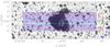 |
Fig. 1 Lines representing the slit positions over a J-band image of N 49 from the SERC survey, obtained with the ALADIN software from the Centre de Données Astronomiques de Strasbourg. The green line identifies the slit on which the reference star (rounded by red ticks) lies. Slit widths are not to scale. |
Data reduction was carried out using IRAF1. The process primarily included overscan and bias subtraction, flat-field correction, and cleaning from cosmic-ray hits. A total of 112 apertures (2″ wide each) were extracted from each 29 2D spectrum. This procedure produced 3248 apertures (1D spectra). The 1D spectra were then wavelength and flux calibrated. Flux calibration was made using a sensitivity function derived from observations of the spectrophotometric standard star Feige 110 (α = 23h19m58.4s, δ = −05°09′56.2″; J2000). These observations were taken each night with the slit aligned to the parallactic angle and widened to 3.0″. Sky correction was conducted by subtracting an average spectrum of about a dozen apertures that had no object emission; these were typically the easternmost apertures. Figure 2 presents the spectrum of an aperture that represents a bright portion of the remnant, 74″ of from the reference star. Emission line fluxes were finally measured from these spectra by Gaussian fitting of the line profile with a continuum baseline defined by eye using the splot/IRAF task. We were unable to resolve red and blue components, therefore the measured fluxes correspond to the integrated value of both. The formal Poissonic errors in the intensities of the strongest lines are calculated to be about 1% on the brightest areas. These estimates are clearly underestimated because errors introduced by the definition of the level of the continuum non-Gaussian form of the line and contribution of blends are neglected. Unfortunately, we were unable to estimate the errors from statistics of different measurements since there is only one exposure for each position.
Some criteria were applied to distinguish real emission lines from noise features. First, the flux must be greater than 1 × 10-18 erg cm-2 s-1, which is about the lower limit of the dynamic range of the measurements. Second, the feature peak value must be greater than 2.5 times the dispersion of the continuum (2.5σ) in the vicinity of the feature.
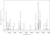 |
Fig. 2 Spectrum of the aperture at 74″ east of the reference star. |
3. Results
3.1. Flux maps
A total of 67 optical emission lines were measured in the final spectra. Some of the brightest emission lines (such as Hα and [O iii] λ5007) were present in about 2000 spectra (pixels on the maps), corresponding to positions over the remnant and beyond it. About 40 lines were mapped at least in the optical region of the remnant.
Derived Hα and [O iii] λ5007 observed flux maps are shown in Fig. 3. These maps show some interesting structures of the remnant, such as the central cavity (around offsets 50″ east and 04″ north) and the faint western boundaries. These boundaries were also visible in images of N 49 presented by Vancura et al. (1992). The boundary in the Hα map is farther from the remnant center than that in the [O iii] map. The northwestern bright region beyond the 10″ western offset seen in the Hα map is a portion of the H ii region DEM L 181. White pixels represent regions without measurements, which generally means that the feature was absent or very weak, and was therefore rejected by the criteria previously explained.
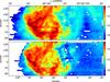 |
Fig. 3 Maps of the observed Hα (top) and [O iii] λ5007 (bottom) fluxes (in logarithmic scale and in units of erg cm-2 s-1). The red cross marks the reference star position (α = 05h25m51.6s, δ = −66°05′05.5″; J2000). Axes indicate the offsets (in arcsec) of the reference star. North is at the top and east is to the left. Each pixel represents a 2″×2″ region on the plane of the sky. |
Many iron lines in different ionization levels were mapped, especially [Fe ii] lines. The presence of strong iron lines is a characteristic of shock-energized objects because shocks are able to destroy grains. Because of this, the iron line intensities can be up to 100 times stronger than in photoionized regions. Dopita et al. (2016) presented the results of an optical integral-field spectroscopy of N 49. Based on emission maps of different [Fe ii], [Fe iii], [Fe v], [Fe x], and [Fe xiv] lines, they have detected a segregation of the different ionic states of iron that cannot be interpreted as a mere projection effect.
Figure 4 shows [Fe xiv] λ5303 (the highest ionization line mapped) and [N i] λ5199 flux maps (one of the low-ionization lines measured). As expected, these maps reveals that the bright features in each map are not spatially coincident, but complementary to a certain degree. The reason is that the emission of these lines originates from very different ionization regions. Emission of [Fe xiv] λ5303 is found throughout almost the entire extension of the remnant, indicating that fast shocks (vs>360 km s-1) are present throughout the nebula (Dopita & Mathewson 1979).
3.2. Line intensity ratio maps
This section presents a set of line flux ratios to Hα or Hβ maps of N 49 (Figs. 5 and 6). Flux ratio maps are interesting because they reveal features of the observed object that are mostly unrelated with its flux maps, as was also seen by Hester et al. (1983) in their photometric maps of the Galactic SNR Cygnus Loop. N 49 ratio maps were overlaid with contours of the Hα flux to allow matching features in different maps. Many ratio maps present some organized spatial variations that certainly are related to variations of one or more physical conditions in the remnant.
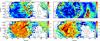 |
Fig. 5 Line ratio to Hα or Hβ maps for strong lines. Values are presented in linear scale. Contours correspond to 5.0×10⁻¹⁴, 8.0×10⁻¹⁵, 3.9× 10⁻¹⁶, and 1.3×10⁻¹⁶ erg cm-2 s-1 from the Hα flux map. To highlight the changes in the line ratios and mitigate outlier effects, the limits of the color scale are the 3% and 97% percentiles. |
Fesen et al. (1982) analyzed ratios of flux to Balmer lines in different portions of the Cygnus Loop and found that line ratios with high-ionization lines (such as [O iii], [Ne iii], and [Ar iii]) are correlated with each other and anticorrelated with line ratios of low-ionization lines ([O i], [N i], [S ii], and so on). The [O ii] λ3727/Hβ, [O iii] λ5007/Hα, [N ii] λ6583/Hα, and [S ii] (λ6716+λ6731)/Hα ratio maps of N 49 are presented in Fig. 5. The first two maps show an outside ring with high values that seems to trace the limits of the remnant. In the [O ii] λ3727/Hβ ratio map, this ring is better defined at the western boundary. The ring structure is complete in the [O iii] λ5007/Hα map, which also shows a trail of high ratio values between the center and the northwestern region that is coincident with the contour of the remnant’s brightest optical limits (between the offsets 40″ east and 22″ east).
Another interesting region becomes prominent in the [N ii] λ6583/Hα map. An area with high values of this ratio starts from the SNR center and extends to its northwestern limits. The [N ii] λ6583/Hα values are about 0.23 at ordinary positions into the nebula, but reach values of up to 1.4 at the external edge of this area. Figure 7 presents spectra from these regions. The intensities of nitrogen emission-lines are strongly correlated with the abundance of this element (Levenson et al. 1995). The [N i] λ5199/Hβ map (shown in Fig. 6 along with other selected flux ratio maps) also presents high values at exactly the same region of highest [N ii] λ6583/Hα values, but the inner part of the remnant in unremarkable. The lack of high [N i] λ5199/Hβ in the internal segment of the area may be caused by nitrogen being mostly ionized to N+ there. However, in the outer part of this area both [N i] and [N ii] are intense, indicating an overabundance of nitrogen there. This nitrogen-rich area might have come from the supernova ejecta or from the wind of the pre-supernova star.
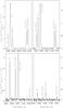 |
Fig. 7 Sections of the spectra including the lines [N ii] λ6583 and [N i] λ5199 from an ordinary position in the remnant (offsets 20″ north and 42″ east, left panels) and from a position with high [N ii]/Hα (offsets 20″ north and 30″ east, right panels). |
The ratio of [S ii] (λ6716+λ6731) to Hα (Fig. 5) presents a radial decrease from the center to the borders. The lowest values of about 0.3 are found on a ring that is coincident with the ring of upper [O iii] λ5007/Hα values located at the border of the SNR. Outside this ring, especially toward the southeast, the ratio [S ii]/Hα increases again. This characteristic is also observed in the [O i] λ6300/Hα map. The line emission from low-ionization ions such as S+ and O0 from this region comes from the photodissociation region associated with N 49. Molecular emission is strong to the southeast of the SNR (Seok et al. 2012), indicating the presence of a molecular cloud. The area in the northwest of this ring is part of the neighbor H ii region DEM L 181.
Other authors also obtained ratio maps of [O iii] λ5007/Hα and [S ii] (λ6716+λ6731)/Hα for N 49, but using imaging techniques (Vancura et al. 1992; Bilikova et al. 2007). The main structures in each ratio map from different works, especially the radial variations, are compatible. Although the spacial resolution of our maps are lower, the spatial coverage toward the west and sensitivity are higher. The range of values obtained by Bilikova et al. (2007) for the ratio of [S ii] (λ6716+λ6731) to Hα (0.4 to 1.4) is very similar to the obtained here (0.3 to 1.2), although our highest [O iii] λ5007/Hα value (1.8) is lower than that found in their higher resolution maps (up to 2.5). In this case, the lower spacial resolution of the new map may be smoothing the higher values, which are claimed by them to be related to the small offset (0.5″) between the emission peaks of [O iii] λ5007 and Hα lines compared to the pixel size (2″). Our new ratio maps in Fig. 6 reveal that radial variations observed on previous ratio maps are also present in many others. In general, ratio maps of low-ionization lines relative to Balmer lines show a radial gradient increasing toward the center, while high ionization line ratio maps show the opposite. A clear exception is the [Fe xiv] λ5303/Hβ map. The highest ratio values are found in regions where almost all the flux maps fade, which are some regions in the internal cavity and the northern and southern extremes of the maps, in accordance to the same ratio map obtained by Dopita & Mathewson (1979). This is expected since these lines are produced in regions that are not spatially coincident: [Fe xiv] λ5303 is emitted from a coronal hot plasma (Te ~ 106 K) while the other lines come from cooler regions (Te ~ 104 K).
An area with high [O iii] λ5007/Hα is located to the southwest. The flux maps in Fig. 3 show that it follows the changes of the Hα intensities, while the [O iii] map is relatively uniform there. Although this region lies outside the remnant, the western side of the remnant has very low densities. This may be allowing a radiation flux to reach this region and generating strong [O iii] λ5007/Hα.
3.3. Extinction
Balmer decrements Hα/Hβ, Hγ/Hβ, and Hδ/Hβ can be used to determine the logarithmic extinction coefficient, c(Hβ), in ionized nebulae, since they are weakly influenced by other physical conditions than the extinction itself. In photoionized nebulae, the intrinsic values of these ratios are about 2.85, 0.47, and 0.26 for an electron temperature of 104 K, electron density of ~103 cm-3 and a case B situation, respectively (Osterbrock & Ferland 2006). When shocks take place, as in SNRs and active galactic nuclei, the collisional excitation of hydrogen Balmer lines should not be negligible and the intrinsic values of the line ratios may change. Because of its lower threshold energy, Hα is more likely to be produced by collisions than Hβ (Hβ is more likely to be produced than Hγ, and so on). This is why many authors used an intrinsic Hα/Hβ of about 3.0 (5% higher than the pure recombination value) when this condition is present (Shull & McKee 1979). We used this value to obtain the c(Hβ) from the Hα/Hβ ratio and the photometric intrinsic values for the other Balmer ratios, because they are less affected.
 |
Fig. 8 Map of Hα to Hβ. |
The Hα/Hβ ratio map shown in Fig. 8 reveals an almost complete ring-like structure with higher values at the object borders (Hα/Hβ~ 4.0). A possible scenario that might generate this feature would be the existence of a high dust concentration in the remnant periphery. The dust would be pushed outward by the expanding ejected gas. This scenario is less likely because we would expect a higher extinction in the southwest region, where the molecular cloud lies. Another possibility considers additional Hα emission that is due to collisional excitation. The high Hα/Hβ ring matches the limits of the remnant reasonably well(even at the fainter western side), which may be an evidence that this ratio traces the forward shock wave front. When the Hα line is collisionally produced, but this ignored (by assuming an intrinsic ratio Hα/Hβ = 2.85), the result should be that any c(Hβ) estimate from the Hα/Hβ ratio would be higher than the derived from the Hγ/Hβ. Instead, the extinction values obtained from Hα/Hβ (intrinsic ratio 2.85) are generally lower than those obtained from the Hγ/Hβ ratio (the difference is even greater if 3.0 is assumed as the intrinsic ratio). This was also observed by Dennefeld (1986) at the same SNR, who ignored any collisional contribution to Hα for this reason.
Models of Shull & McKee (1979) predict a Hα/Hβ ratio up to 4.2 (corresponding to a collisional excitation contribution of ~30%). Typical Hα/Hβ at the borders of N 49 are only 15% higher than the overall mean. This shows that recombination is the chief mechanism of Hα and Hβ line emission in whole SNR, and the collisional excitation may be responsible for the increase in the Hα/Hβ ratio at the borders.
3.4. Extinction correction
To obtain best temperature estimates, fluxes were corrected for extinction effects using results previously presented. Lines with wavelengths larger than Hβ were corrected using c(Hβ) from Hα/Hβ. Lines with wavelengths smaller than Hδ were corrected considering the c(Hβ) values obtained from Hδ/Hβ. The correction for those lines with wavelengths between Hδ and Hβ considered c(Hβ) values calculated from Hγ/Hβ. When a pixel had no extinction estimate for one Balmer ratio, the c(Hβ) from the nearest Balmer line was adopted.
3.5. Electron density and temperature
The [O iii] λ4363 and [O ii] λ7320, 30 lines are blended with [Fe ii] λ4359 and [Ca ii] λ7325. We deblended them by subtracting the undesired line flux from each blend, which we calculated from other lines of the same ion for which theoretical relative intensities are known. The [Ca ii] λ7325 line flux was obtained from the [Ca ii] λ7291, whose relative intensities are I(λ7291)/I(λ7325) = 3/2 (Fesen et al. 1982). The [Fe ii] λ4359 intensity could not be calculated directly in all the pixels where the blend [O iii]+[Fe ii] was measured since the [Fe ii] λ4287 was not measured in all pixels. To solve this, we combined the spectra of these pixels (in groups of about 10) according to their ([O iii]+[Fe ii])/Hβ value. The ([O iii]+[Fe ii])/[Fe ii] λ4287 ratio of the combined spectra was used to derive the [Fe ii] λ4287 from direct comparison with the [O iii]+[Fe ii] value in the pixels where [Fe ii] λ4287 was missing. Then the [Fe ii] λ4359 line flux map was built using the theoretical ratio of I(λ4287)/I(λ4359) ~ 3/2 (Garstang 1962).
Electron density and temperature maps were obtained iteratively. The density was estimated from the line ratio [S ii] λ6716/ λ6731 and the temperature from [S ii] (λ6716 + λ6731)/(λ4069 + λ4076), [O iii] (λ5007+λ4959)/λ4363, [O ii] λ3727/λ7325, and [N ii] (λ6548+λ6583)/λ5755. The mean value over the map of one property was used to recalculate the other for pixels where the first had no value due to the lack of measured lines. Iterations were repeated until differences between pixel values in consecutive maps were smaller than 10%.
Figure 9 shows the electron density map derived from the [S ii] λ6716 /λ6731 ratio. The electron density map is consistent with previous studies, especially with that from Melnik & Copetti (2013), where the increase in the density toward the southeast region was detected. The better spatial resolution and larger covered region of our data allow for a more detailed density map, however. For example, our density map shows that high-density values (> 2000 cm-3) are found outside the remnant’s brightest region, around offsets 92″ east and 4″ south. The overall variation in density is smooth, with a continuous increase in density from northwest to southeast, but in some positions local density peaks are found. Figure 11 shows the density histogram.
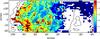 |
Fig. 9 Electron density maps in units of 103 cm-3. |
Temperature maps from [S ii] (λ6716 + λ6731)/(λ4069 + λ4076), [O iii] (λ5007+λ4959)/λ4363, [O ii] λ3727/λ7325, and [N ii] (λ6548+λ6583)/λ5755 line ratios are presented in Fig. 10. The last three temperature maps were calculated assuming the electron density values obtained in the previous process. Histograms of the electron density and temperature are presented in Figs. 11 and 12. The temperature distribution throughout the remnant is different among different temperature maps. In the [S ii] temperature map, values seem to increase toward the borders, while [O iii] temperatures reach the highest values near the center. The [O ii] electron temperature map shows higher values in the western half. Higher values of [N ii] temperatures are found for some pixels at the northeastern edge of N 49. The [N ii] electron temperature map does not show values in the high [N ii] (λ6548+λ6583)/Hα area because the [N ii] λ5755 line is absent. The absence of [N ii] λ5755 emission in this regions surely does not result from a low ionic abundance, since [N ii]λ6583 line is intense there. Therefore, the faintness of the line indicates a low temperature in this area.
Although the temperature change in different maps is not the same, mean values are similar (about 1.1 × 10⁴ K) for the [S ii], [O ii], and [N ii] temperatures. Higher values are found in the [O iii] temperature map, with a mean value of about 3.7 × 10⁴ K (this value would be about 5.0 × 10⁴ K if the [O iii] λ4363 line would not have been deblended).
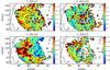 |
Fig. 10 Electron temperature maps for the [S ii], [O iii], [O ii] and [N ii] line ratios. Electron temperature unit is 103 K. |
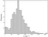 |
Fig. 11 Histogram of the electron density. The statistics used 1400 values. |
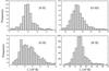 |
Fig. 12 Histograms of the electron temperature for different temperature-sensitive line ratios. The statistics for the [S ii], [O iii], [O ii], and [N ii] temperatures used 686, 710, 705, and 492 values, respectively. |
3.6. Density and temperature estimations from the integrated spectrum compared with published data
We combined spectra from the 800 brightest regions in the remnant to generate one spectrum with a high signal-to-noise ratio. Flux measurements from the integrated spectrum were used to obtain electron density, temperature, and extinction estimates as overall results for N 49. Results are presented in Table 1 along with dereddened flux ratio values from published data on N 49 and properties recalculated from them. Calculation for properties from the integrated spectrum followed the same steps as those for the maps. Density values are around 103 cm-3 for most works. The higher values for Vancura et al. (1992) and Russell & Dopita (1990) arise because the observed region is in the southwest. Our [O iii] temperature value is between those determined by Vancura et al. (1992) and Osterbrock & Dufour (1973). Temperatures for other line ratios are between 8.5×10³ K to 1.3×10⁴ K for all authors. Extinction results from different works do not agree perfectly. Our extinction determinations from Hγ/Hβ and Hδ/Hβ are higher than those of Hα/Hβ. Dennefeld (1986) data imply the same, but Russell & Dopita (1990) data show the opposite.
Properties derived from the integrated spectrum and recalculated using line ratio values from published data.
4. Discussion
Many line ratios in Figs. 5 and 6 present a radial variation with values increasing toward the central region (e.g. Ca ii λ3934/Hβ, [O i] λ6300/Hα, and [S ii] λλ6716,31/Hα) or toward the borders ([Ne iii] λ3869/Hβ, [O iii] λ5007/Hβ, and [Ar iii] λ7136/Hα, for example). Figure 13 shows radial profiles of line ratio intensities obtained by averaging in 2″ wide concentric annuli and normalizing to the value at radius 15″. We investigated this behavior by ordering these lines so that the ratio of each line to the next increases toward the borders. For example, [O iii] λ5007/Hβ, and [Ne iii] λ3869/Hβ maps have higher values at the borders, but the [O iii] λ5007/[Ne iii] λ3869 map also does. This places the [O iii] λ5007 line before the [Ne iii] λ3869 in this order. We concluded that the ratio of two lines L1/L2 is positively correlated with the distance from the center when L1 comes before L2 in the sequence: [O iii] λ5007, [O iii] λ4363, [Ar iii] λ7136, [Ne iii] λ3869, [O ii] λ7325, [O ii] λ3727, He ii λ4686, Hβ λ4861, [N ii] λ6583, He i λ6678, [S ii] λ6731, [S ii] λ6716, [O i] λ6300, [Ca ii] λ7291, Ca ii λ3934, and [N i] λ5199. The greater the distance between two lines in this list, the stronger the variation with distance of their ratio.
A sequence of lines very similar to the one of the previous paragraph can be obtained from the MAPPINGS III code by analyzing how line ratios change as the shock velocity changes. Figure 14 presents interpolated curves for different line ratios (to Hβ) modeled by the code for a shock component. Line ratios are normalized to their values at vs = 150 km s-1. This plot shows that, according to the rate of increase with the shock velocity, the considered line ratios follow a sequence very similar to that obtained from the correlation analysis that we showed in Fig. 13. When the shock velocity decreases from 300 km s-1 to lower values, line ratios such as [O iii] λ5007/Hβ and [Ne iii] λ3869/Hβ increase and those of [N ii] λ5199/Hβ and Ca ii λ3934 decrease. These changes are the same as those observed in line ratio maps with increasing distance from the remnant center, meaning that regions farther from the center would have lower velocities.
According to MAPPINGS III data, for velocities lower than ~150 km s-1, some line ratios invert their variation when the shock velocity decreases. For example, [O iii] λ5007/Hβ starts to decrease when the shock velocity decreases when values are lower than ~150 km s-1 and, on the other hand, [N ii] λ5199/Hβ increases in this velocity regime with decreasing shock velocity. Velocities this low may be occurring specially on the very edge of the remnant, where the sharp ring structure is seen (as those found on [O iii] λ5007/Hβ and [S ii] (λ6716+λ6731)/Hα maps). The ring structure in each map may be indicating where the specific shock velocity on which the line ratio behavior (when the shock velocity varies) inverts is predominant.
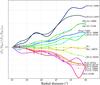 |
Fig. 13 Profiles of line ratio maps. Points represent mean values for each line ratio (to Hβ) in 2″ concentric annuli, normalized to the value at radius 15″. Lines represent interpolated curves. |
 |
Fig. 14 Line ratios to Hβ λ4861 versus shock velocity according to the MAPPINGS III code for LMC abundances, magnetic field strength of 10-4μG and an ambient density of 1 cm-3 for the shock component only. Points are numeric data and lines represent interpolated curves. Values are normalized to their results for vs = 150 km s-1. Colors identifying each line ratio are the same as in Fig. 13. |
Many line ratios have almost constant modeled values for shock velocities higher than about 300 km s-1. If shock velocity changes are indeed responsible for the radial variations in line ratio maps, then shocks slower than 300 km s-1 would be required. This is in accordance with results from Vancura et al. (1992), who concluded that shock velocities are mainly in the interval of 40–270 km s-1. Bilikova et al. (2007) also reported that velocities in N 49 are about 250 km s-1 for dense clouds and lower than 300 km s-1 for low density regions.
Melnik & Copetti (2013) showed that the kinematics and morphology of N 49 cannot be explained by a simple projection effect of a spherical shell and, surprisingly, that the gas velocity, v, and distance from the center, r, are related by v(r) = r-0.9. However, a systematic dependence of the shock velocity on radius is not expected, even for a clumpy medium. The radial variation of line ratios is related to the time-dependency of cooling and ionization processes, and this might be the reason for the coincidence between the sequences of line ratios obtained from the radial profiles (Fig. 13) and from MAPPINGS curves of line strength versus shock velocity (Fig. 14).
5. Conclusions
We presented a set of maps of line fluxes and line flux ratios for N 49, along with derived electron density, temperature, and extinction maps. Our analysis and conclusions are summarized below.
-
1.
Line flux maps were built for 67 differentemission lines. About 40 maps have fluxmeasurements at least in the brightest optical region ofN 49. Many line ratio maps relative to Balmerlines presented radial variations.
-
2.
We found an area of high [N ii] λ6583/Hα values in this ratio map. This area extends from the center to the northwestern N 49 border, where the high ratio values (~1.4) compared to other positions in the remnant (~0.23) are found. Since this line ratio is highly sensitive to the elemental abundance, we suggest that the intense [N ii] emission probably arises from a nitrogen-rich material that is expelled from the progenitor star in the explosion or as a wind in the pre-supernova phase.
-
3.
Extinction estimates were obtained using the line ratios Hα/Hβ, Hγ/Hβ, and Hδ/Hβ. A ring structure around the remnant observed in the Hα/Hβ maps suggests that Hα emission has a contribution of about 30% from collisional excitation in this region.
-
4.
The electron density map was built using the [S ii] λ6716/λ6731 line ratio. Many high values are found beyond the brightest southwest region of N 49. The electron temperature was obtained using [S ii], [O ii], [O iii], and [N ii]. Values from single ionized ions are about 1.1×10⁴ K and 3.6×10⁴ K for [O iii]. Temperature variation patterns are different in maps from different temperature-sensitive line ratios.
-
5.
We investigated the variation of line ratios with distance from the remnant center. MAPPINGS III models (Allen et al. 2008) show that different line ratios depend differently on the shock velocity. The way line ratios vary and how sensitive to velocity variations each ratio is matches our observational data if we assume that the shock speed decreases toward the remnant border. However, the required dependence of the shock velocity on radius is unexpected. The time-dependency of cooling and ionization processes may be the cause of the spatial variation in the line ratios.
IRAF is distributed by the National Optical Astronomy Observatory, which is operated by the Association of Universities for Research in Astronomy (AURA) under cooperative agreement with the National Science Foundation.
Acknowledgments
We wish to thank the SOAR staff, in particular Tina Armond, who obtained the spectroscopic data. This work was supported by the Brazilian agencies CAPES and CNPq.
References
- Alikakos, J., Boumis, P., Christopoulou, P. E., & Goudis, C. D. 2012, A&A, 544, A140 [NASA ADS] [CrossRef] [EDP Sciences] [Google Scholar]
- Allen, M. G., Groves, B. A., Dopita, M. A., Sutherland, R. S., & Kewley, L. J. 2008, ApJS, 178, 20 [Google Scholar]
- Banas, K. R., Hughes, J. P., Bronfman, L., & Nyman, L.-A. 1997, ApJ, 480, 607 [NASA ADS] [CrossRef] [Google Scholar]
- Bilikova, J., Williams, R. N. M., Chu, Y.-H., Gruendl, R. A., & Lundgren, B. F. 2007, AJ, 134, 2308 [NASA ADS] [CrossRef] [Google Scholar]
- Chevalier, R. A. 1977, ARA&A, 15, 175 [NASA ADS] [CrossRef] [Google Scholar]
- Dennefeld, M. 1986, A&A, 157, 267 [NASA ADS] [Google Scholar]
- Dickel, J. R., Chu, Y.-H., Gelino, C., et al. 1995, ApJ, 448, 623 [NASA ADS] [CrossRef] [Google Scholar]
- Dopita, M. A., & Mathewson, D. S. 1979, ApJ, 231, L147 [NASA ADS] [CrossRef] [Google Scholar]
- Dopita, M. A., Blair, W. P., Long, K. S., et al. 2010, ApJ, 710, 964 [NASA ADS] [CrossRef] [Google Scholar]
- Dopita, M. A., Seitenzahl, I. R., Sutherland, R. S., et al. 2016, ApJ, 826, 150 [NASA ADS] [CrossRef] [Google Scholar]
- Fesen, R. A., Blair, W. P., & Kirshner, R. P. 1982, ApJ, 262, 171 [NASA ADS] [CrossRef] [Google Scholar]
- Garstang, R. H. 1962, MNRAS, 124, 321 [NASA ADS] [Google Scholar]
- Hester, J. J., Parker, R. A. R., & Dufour, R. J. 1983, ApJ, 273, 219 [NASA ADS] [CrossRef] [Google Scholar]
- Levenson, N. A., Kirshner, R. P., Blair, W. P., & Winkler, P. F. 1995, AJ, 110, 739 [NASA ADS] [CrossRef] [Google Scholar]
- McKee, C. F., Cowie, L. L., & Ostriker, J. P. 1978, ApJ, 219, L23 [NASA ADS] [CrossRef] [Google Scholar]
- Melnik, I. A. C., & Copetti, M. V. F. 2013, A&A, 553, A104 [NASA ADS] [CrossRef] [EDP Sciences] [Google Scholar]
- Osterbrock, D. E., & Dufour, R. J. 1973, ApJ, 185, 441 [NASA ADS] [CrossRef] [Google Scholar]
- Osterbrock, D. E., & Ferland, G. J. 2006, Astrophysics of gaseous nebulae and active galactic nuclei, eds. D. E. Osterbrock, & G. J. Ferland (Sausalito, CA: University Science Books) [Google Scholar]
- Raymond, J. C., Blair, W. P., Fesen, R. A., & Gull, T. R. 1983, ApJ, 275, 636 [NASA ADS] [CrossRef] [Google Scholar]
- Russell, S. C., & Dopita, M. A. 1990, ApJS, 74, 93 [NASA ADS] [CrossRef] [Google Scholar]
- Seok, J. Y., Koo, B.-C., & Onaka, T. 2012, ApJ, 744, 160 [NASA ADS] [CrossRef] [Google Scholar]
- Shull, J. M., & McKee, C. F. 1979, ApJ, 227, 131 [NASA ADS] [CrossRef] [Google Scholar]
- Vancura, O., Blair, W. P., Long, K. S., & Raymond, J. C. 1992, ApJ, 394, 158 [NASA ADS] [CrossRef] [Google Scholar]
- Williams, R. M., Chu, Y.-H., Dickel, J. R., et al. 1999, ApJS, 123, 467 [NASA ADS] [CrossRef] [Google Scholar]
- Woltjer, L. 1972, ARA&A, 10, 129 [NASA ADS] [CrossRef] [Google Scholar]
All Tables
Properties derived from the integrated spectrum and recalculated using line ratio values from published data.
All Figures
|
Fig. 1 Lines representing the slit positions over a J-band image of N 49 from the SERC survey, obtained with the ALADIN software from the Centre de Données Astronomiques de Strasbourg. The green line identifies the slit on which the reference star (rounded by red ticks) lies. Slit widths are not to scale. |
| In the text | |
|
Fig. 2 Spectrum of the aperture at 74″ east of the reference star. |
| In the text | |
|
Fig. 3 Maps of the observed Hα (top) and [O iii] λ5007 (bottom) fluxes (in logarithmic scale and in units of erg cm-2 s-1). The red cross marks the reference star position (α = 05h25m51.6s, δ = −66°05′05.5″; J2000). Axes indicate the offsets (in arcsec) of the reference star. North is at the top and east is to the left. Each pixel represents a 2″×2″ region on the plane of the sky. |
| In the text | |
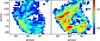 |
Fig. 4 Same as Fig. 3 for [Fe xiv] λ5303 (left) and [N i] λ5199 (right) lines. |
| In the text | |
|
Fig. 5 Line ratio to Hα or Hβ maps for strong lines. Values are presented in linear scale. Contours correspond to 5.0×10⁻¹⁴, 8.0×10⁻¹⁵, 3.9× 10⁻¹⁶, and 1.3×10⁻¹⁶ erg cm-2 s-1 from the Hα flux map. To highlight the changes in the line ratios and mitigate outlier effects, the limits of the color scale are the 3% and 97% percentiles. |
| In the text | |
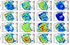 |
Fig. 6 Same as Fig. 5 for a sample of medium-intensity lines relative to Hα or Hβ. |
| In the text | |
|
Fig. 7 Sections of the spectra including the lines [N ii] λ6583 and [N i] λ5199 from an ordinary position in the remnant (offsets 20″ north and 42″ east, left panels) and from a position with high [N ii]/Hα (offsets 20″ north and 30″ east, right panels). |
| In the text | |
|
Fig. 8 Map of Hα to Hβ. |
| In the text | |
|
Fig. 9 Electron density maps in units of 103 cm-3. |
| In the text | |
|
Fig. 10 Electron temperature maps for the [S ii], [O iii], [O ii] and [N ii] line ratios. Electron temperature unit is 103 K. |
| In the text | |
|
Fig. 11 Histogram of the electron density. The statistics used 1400 values. |
| In the text | |
|
Fig. 12 Histograms of the electron temperature for different temperature-sensitive line ratios. The statistics for the [S ii], [O iii], [O ii], and [N ii] temperatures used 686, 710, 705, and 492 values, respectively. |
| In the text | |
|
Fig. 13 Profiles of line ratio maps. Points represent mean values for each line ratio (to Hβ) in 2″ concentric annuli, normalized to the value at radius 15″. Lines represent interpolated curves. |
| In the text | |
|
Fig. 14 Line ratios to Hβ λ4861 versus shock velocity according to the MAPPINGS III code for LMC abundances, magnetic field strength of 10-4μG and an ambient density of 1 cm-3 for the shock component only. Points are numeric data and lines represent interpolated curves. Values are normalized to their results for vs = 150 km s-1. Colors identifying each line ratio are the same as in Fig. 13. |
| In the text | |
Current usage metrics show cumulative count of Article Views (full-text article views including HTML views, PDF and ePub downloads, according to the available data) and Abstracts Views on Vision4Press platform.
Data correspond to usage on the plateform after 2015. The current usage metrics is available 48-96 hours after online publication and is updated daily on week days.
Initial download of the metrics may take a while.