| Issue |
A&A
Volume 594, October 2016
|
|
|---|---|---|
| Article Number | A67 | |
| Number of page(s) | 18 | |
| Section | The Sun | |
| DOI | https://doi.org/10.1051/0004-6361/201628913 | |
| Published online | 13 October 2016 | |
Impact of flux distribution on elementary heating events
School of Mathematics and Statistics, University of St Andrews, North Haugh, St Andrews, Fife, KY16 9SS, UK
e-mail: This email address is being protected from spambots. You need JavaScript enabled to view it.
Received: 12 May 2016
Accepted: 23 June 2016
Abstract
Context. The complex magnetic field on the solar surface has been shown to contain a range of sizes and distributions of magnetic flux structures. The dynamic evolution of this magnetic carpet by photospheric flows provides a continual source of free magnetic energy into the solar atmosphere, which can subsequently be released by magnetic reconnection.
Aims. We investigate how the distribution and number of magnetic flux sources impact the energy release and locations of heating through magnetic reconnection driven by slow footpoint motions.
Methods. 3D magnetohydrodynamic (MHD) simulations using Lare3D are carried out, where flux tubes are formed between positive and negative sources placed symmetrically on the lower and upper boundaries of the domain, respectively. The flux tubes are subjected to rotational driving velocities on the boundaries and are forced to interact and reconnect.
Results. Initially, simple flux distributions with two and four sources are compared. In both cases, central current concentrations are formed between the flux tubes and Ohmic heating occurs. The reconnection and subsequent energy release is delayed in the four-source case and is shown to produce more locations of heating, but with smaller magnitudes. Increasing the values of the background field between the flux tubes is shown to delay the onset of reconnection and increases the efficiency of heating in both the two- and four-source cases. The cases with two flux tubes are always more energetic than the corresponding four flux tube cases, however the addition of the background field makes this disparity less significant. A final experiment with a larger number of smaller flux sources is considered and the field evolution and energetics are shown to be remarkably similar to the two-source case, indicating the importance of the size and separation of the flux sources relative to the spatial scales of the velocity driver.
Key words: Sun: corona / Sun: magnetic fields / Sun: activity / magnetohydrodynamics (MHD)
© ESO, 2016
1. Introduction
A long-standing problem in solar physics is understanding the energy transportation from the photosphere and subsequent dissipation in the solar atmosphere, to account for the high temperatures, of over a million degrees Kelvin, that are observed in the solar corona.
The magnetic field, permeating the Sun’s atmosphere, plays a crucial role in both the energy transportation and deposition and a variety of heating mechanisms have been suggested to account for the energy release in the solar atmosphere. One group of theories proposes that velocities, produced by the internal convection and turbulent motions of the Sun, slowly (compared to the Alfvén speed) advect the footpoints of the coronal magnetic field on the solar surface, enabling energy to be stored in the magnetic field as current concentrations. In a series of papers by Parker (Parker 1972, 1979, 1994) it was proposed that the subsequent magnetic reconnection and dissipation of many current sheets (tangential discontinuities) in the solar atmosphere could lead to the observed coronal temperatures.
Parker (1972) suggested that a uniform field that is subjected to highly complex velocity patterns at the footpoints, would lead to the creation of these current sheets and the subsequent energy dissipation. This is known as the theory of field line braiding and is also hypothesised as being associated with the localised impulsive energy events known as nanoflares (Parker 1988) observed in the corona. A range of numerical simulations (e.g. Ballegooijen 1988; Galsgaard & Nordlund 1996; Longcope & Sudan 1994; Rappazzo et al. 2007, 2008; Ng et al. 2012; Wilmot-Smith 2015), using various velocity drivers, have been carried out to examine Parker’s theory of braiding, with an emphasis on the analysis of the formation of current concentrations and the resulting reconnection and energy release.
In Parker’s original model, an initially uniform magnetic field is assumed. However, high resolution observations have shown that the magnetic field protruding from active regions on the solar surface is concentrated into highly complex, intricate configurations (e.g. Title & Schrijver 1998), with structures visible down to the scale of the observational limit. Large features such as coronal loops are therefore also considered as being made up of multiple smaller strands (Brooks et al. 2013; Scullion et al. 2014) that are each rooted to individual flux fragments on the solar surface. This will result in the presence of many topological features, such as separatrix surfaces, that divide different regions of connectivity within the coronal loops. The slow advection of these magnetic field fragments was considered by Priest et al. (2002) in the theory of “coronal tectonics”. Priest et al. argued that only simple velocity motions on the photospheric footpoints of a complex fragmented magnetic field are required to produce current formation along these topological features.
There have been many analytical and numerical investigations (e.g. Lau & Finn 1990; Priest et al. 2003; Baumann et al. 2013; Parnell et al. 2010, 2015; Stevenson et al. 2015) examining the importance of topological features, such as separators and null points as locations for current build up and reconnection to occur. However, it has also been shown that geometrical features, such as quasi-separatrix layers (QSLs; Priest & Démoulin 1995; Démoulin et al. 1996a,b), where the change in connectivity is continuous but very large, are also locations associated with current formation and energy release (e.g. Aulanier et al. 2006; Janvier et al. 2015).
Numerical experiments focusing on simple shearing of photospheric flux patches, emulating the coronal tectonics model, have found that the application of a simple shearing driver to a field with an existing complex geometry created current concentrations and associated heating (Mellor et al. 2005). Extending this idea, a series of simulations by De Moortel & Galsgaard (2006a,b), Wilmot-Smith & De Moortel (2007) went on to examine the elementary heating events produced by the rotation and/or spinning of two flux tubes and found that a current layer was built up along the separatrix surface that separates the two flux tubes. De Moortel & Galsgaard (2006b) then went on to examine the scale of velocity drivers, comparing a large-scale rotation of the magnetic flux sources compared to small-scale spinning of the individual flux tubes, analysing the current formation and subsequent reconnection. These simulations give support to the coronal tectonics model as a viable method for contributing to coronal heating. However, it has yet to be fully explored exactly how the current formation and heating depends on the extent of the complexity of the initial magnetic field configuration, and how the interaction of multiple magnetic loops (strands) can impact the estimated energy release.
In this paper, we consider a series of simplistic flux distributions from which we construct magnetic flux tubes, which we shall subject to the same (rotational) footpoint driving motion, in order to compare how the size, number and distribution of the flux sources impact the current concentrations and the subsequent magnetic reconnection and energy release. The basic model consists of two flux sources (producing two aligned flux tubes), the same initial configuration as in De Moortel & Galsgaard (2006a) and De Moortel & Galsgaard (2006b). We extend this model to consider a four-source case (producing four aligned flux tubes) and then go on to consider a series of cases with further small-scale flux sources with minimal separation.
The remainder of this paper is structured as follows: the numerical code, initial flux tube set-up and the velocity driver are described in Sect. 2. In Sect. 3 the dynamic evolutions and energetics of the experiments are discussed and finally, in Sect. 4, a discussion of the results and conclusions is given.
2. Set-up and boundary conditions
2.1. Numerical code
The numerical experiments are carried out using the 3D magnetohydrodynamic (MHD) code Lare3D (Arber et al. 2001). This is a Lagrangian Remap scheme using a second order accurate predictor-corrector method. The numerical code solves the non-ideal MHD equations given by
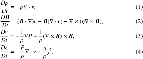 where P is the pressure, ρ is the density, B is the magnetic field, E is the electric field, j is the electric current density, v is the velocity, t is the time and ϵ is the specific internal energy density, given by
 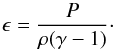 (5)In Lare3D the variable η is the resistivity defined as
  (where σ is the conductivity), not the magnetic diffusivity. The MHD equations have been non-dimensionalised, by choosing normalising values for the magnetic field B0, density ρ0 and length L0. These normalising constants can then be used to retrieve the dimensional values by the following scaling relations
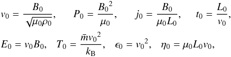 where μ0 is the magnetic permeability of a vacuum (μ0 = 4π × 10-7H m-1 ), kB = 1.3807 × 10⁻²³ J K-1 is the Boltzmann constant and
  is the average mass of ions in the plasma and
  is used, representing pure hydrogen. All the results shall be presented in normalised units, but a normalisation given by: B0 = 100 G, L0 = 75 Mm, ρ0 = 1.67 × 10⁻¹¹ kg m-3 is used to consider the corresponding coronal values.
The simulations are run with a localised non-ideal region, with the resistivity given by 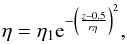 (6)with rη = 0.1 and η1 = 10-4. The resistivity is constant in the x-y plane, with a maximum value in the mid-plane and reduces to zero at the footpoints, to prevent the magnetic sources from diffusing. A comparison was also carried out with cases using a radially dependent sphere of localised resistivity (as used by Pontin et al. 2005). However, with a radially dependent η, resistivity was therefore not present to diffuse the high currents formed by the flux tube formation on the x and y boundaries and the subsequent Lorentz force on the boundaries was shown to impact the evolutions.
The simulations are all carried out with numerical grid points of 5122 in the x and y-direction and 256 in z. The energy conservation was shown to increase with higher resolutions comparing 1283, 2563 and 5123 and was conserved to within 4% for all cases with 5123. However a reduction in the resolution in the z-direction (to 256 grid points) was shown to have little impact on the results (as the majority of the small scales and currents are created in the x−y plane) and required less numerical resources.
There is no uniform viscosity used in the simulations, but an artificial shock viscosity is applied with a corresponding associated heating term in Eq. (4), for which we refer to Arber et al. (2001) for a full description of its implementation in Lare3D (where the shock viscosity parameters used are ν1 = 0.1 and ν2 = 0.5). Conduction, radiation and gravity are also neglected, therefore the simulations are carried out with an initial uniform density.
The MHD equations are solved in a Cartesian box, where the normal derivatives of the magnetic field, energy and density are zero on all the boundaries. On the x and y boundaries the velocity components are also chosen to be zero, while on the z boundaries the velocity components on the upper and lower boundaries are given by the velocity driver, described in Sect. 2.3.
2.2. Flux tubes in numerical equilibrium
The simulations are carried out in a unit cube domain 0.0 <x,y,z< 1.0, in normalised variables. In this paper we shall consider different initial magnetic field configurations, which consist of vertical flux tubes formed between aligned positive sources on the lower boundary and negative sources on the upper boundary. The distribution of the sources on the upper and lower boundaries for a generic case of N sources is given by ![Mathematical equation: \begin{eqnarray} {B}_{z}=\sum_{n=1}^{N} ({B}_{\rm max})_{n}~{\rm e}^{-[(x-{(xs)}_{n})^2+(y-{(ys)}_{n})^2]/{{(rs)}_{n}^2}} + {B}_{\rm Bg}, \label{eq:bz_4src_bg} \end{eqnarray}](/articles/aa/full_html/2016/10/aa28913-16/aa28913-16-eq45.png) (7)where (Bmax)n and rsn define the peak strength and radius of source n and each is centred at (xsn,ysn). The flux tubes are formed by the numerical relaxation of vertical magnetic field (Bx = By = 0.0 and Bz given by Eq. (7)) towards equilibrium, with a constant density and internal energy. Qualitatively similar to the potential field case, this method produces flux tubes expanding from the concentrated sources on the boundaries and has minimal current in the domain. The final velocities in the domain after the relaxation were also much less than the driving velocity we shall consider in Sect. 2.3.
(7)where (Bmax)n and rsn define the peak strength and radius of source n and each is centred at (xsn,ysn). The flux tubes are formed by the numerical relaxation of vertical magnetic field (Bx = By = 0.0 and Bz given by Eq. (7)) towards equilibrium, with a constant density and internal energy. Qualitatively similar to the potential field case, this method produces flux tubes expanding from the concentrated sources on the boundaries and has minimal current in the domain. The final velocities in the domain after the relaxation were also much less than the driving velocity we shall consider in Sect. 2.3.
We use the term “flux tubes” to refer to the flux associated within the specified radius (rsn) of the sources, as opposed to distinct topological features. Moreover, in the first comparison (in Sect. 3.1) no additional field is added between the flux tubes on the boundaries (Bbg = 0.0) and therefore we note that these numerical experiments are near the computational limit of producing separators, however, we shall refer to the mapping of the field lines on the boundary to be continuous (i.e. with a QSL present).
2.3. Velocity driver
The flux tubes are subjected to a driving velocity on the upper and lower boundaries at z = 0.0 and z = 1.0. A rotational velocity is used as in De Moortel & Galsgaard (2006a). The driver on the lower boundary is described by: ![Mathematical equation: \begin{eqnarray} {v}_{x}&=&-{v}_{1}~r~\sin({\theta})~\bigg[1+\tanh\bigg(A~(1-B~r)\bigg)\bigg],\nonumber \\ {v}_{y}&=& ~~{v}_{1}~r~\cos({\theta})~\bigg[1+\tanh\bigg(A~(1-B~r)\bigg)\bigg], \label{eq:vel_driver1} \end{eqnarray}](/articles/aa/full_html/2016/10/aa28913-16/aa28913-16-eq55.png) (8)where
(8)where  (9)This produces a rotational driver in the anti-clockwise direction on z = 0.0, as indicated in Fig. 2a. The velocity is zero in the centre of the plane and increases linearly with the radius from this point. The coefficients A and B describe the steepness and drop off of the driver near the boundaries, respectively, and are set as A = 16.8 and B = 2.8. The coefficient v1 determines the magnitude of the rotation and is chosen to be v1 = 0.02. The velocity profile at z = 1.0 has exactly the same magnitude and profile as at z = 0.0, but in the opposite direction (clockwise). The sources on the top and bottom boundaries are therefore counter rotated, effectively doubling the actual twist (2θ) that the field experiences.
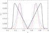 |
Fig. 1 Profile of the imposed driving velocity (black) and profile of Bz (red) and | B | (blue) for the two-source case (i) at z = 0.0 and y = 0.5. |
Figure 1 shows the velocity profile (black) varying with x at y = 0.5 on the lower boundary. Towards the edge of the plane the velocity decreases sharply to reduce shear at the x and y boundaries. To start the rotation smoothly, this driver is built up over time using a tanh profile: ![Mathematical equation: \begin{eqnarray} v=v~\bigg[1+\tanh\bigg(\frac{t-{t}_{1}}{{t}_{\rm d}}\bigg)\bigg]\cdot \end{eqnarray}](/articles/aa/full_html/2016/10/aa28913-16/aa28913-16-eq67.png) (10)This allows the velocity to increase gradually to help reduce waves and shocks from a sudden velocity onset, where the parameters t1 and td are set as 2 and 0.5, respectively.
(10)This allows the velocity to increase gradually to help reduce waves and shocks from a sudden velocity onset, where the parameters t1 and td are set as 2 and 0.5, respectively.
3. Numerical experiments
3.1. Two and four source comparisons
An initial comparison is carried out between cases with two and four flux tubes. The sources on the upper and lower boundaries of the domain for the four flux tube case are centred at (xsA,ysA) = (0.3,0.5), (xsB,ysB) = (0.5,0.7), (xsC,ysC) = (0.7,0.5), and (xsD,ysD) = (0.5,0.3), which we shall call sources A, B, C and D (a,b,c and d) on the lower (upper) boundary for ease of reference (see Fig. 2). Only the sources A (a) and C (c) are present in the two-source case. The sources are positioned within the linear section of the velocity driver, ensuring minimum distortion of the foot points on the boundary (as illustrated in Fig. 1).
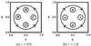 |
Fig. 2 Magnetic source labels at t = 0 on a) z = 0.0 and b) z = 1.0. The direction of rotation is also indicated. |
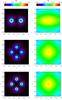 |
Fig. 3 Contour plots of | B | after relaxation at z = 0.0 (left column) and z = 0.5 (right column) for cases with (i) 2 sources (top row); (ii) “weak” 4 sources (middle row) and (iii) “compact” 4 sources (bottom row). |
The two-source case uses Bmax = 1.0 and rsn = 0.065, for both sources, and shall be referred to as case (i). We consider two cases with four sources, which both retain the same total magnetic flux through the surfaces at z = 0.0 and z = 1.0 as case (i). The first case uses the parameter values Bmax = 0.5 and rsn = 0.065. The radius of the sources remains the same as in the two-source case, but the peak magnitude (Bmax) is halved. The second case retains the same peak magnitude but the radius is reduced by a factor of  , where Bmax = 1.0 and rsn = 0.065/. This enables us to compare the original two-source case with four “weaker” sources of the same size (case ii) as well as with four more “compact” sources (case iii). This initial comparison is carried out without a background field (BBg = 0). The resulting magnetic field strength on the lower boundary for the three cases is displayed in the contours in the left column of Fig. 3.
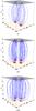 |
Fig. 4 A selection of field lines traced from z = 0.0 for cases i) 2 sources; ii) 4 sources (weak); and iii) 4 sources (compact). |
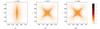 |
Fig. 5 Projected Lorentz force in the plane (arrows) over-plotted on contours of the magnitude of the current density in the mid-plane between 0.25 <x,y< 0.75 at t = 50 for case i) 2 sources; and at t = 60 for cases ii) 4 weak sources and iii) 4 compact sources. |
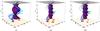 |
Fig. 6 A selection of field lines traced from source C on z = 0 at t = 60 for cases i) 2 sources; ii) 4 weak sources and iii) 4 compact sources, coloured according to their connectivity. Over-plotted are the isosurfaces of the current density of magnitude 2.5 within the central box (0.1 <x,y,z< 0.9) in the domain. |
Using these boundary conditions the flux tubes are created in the three cases using the numerical relaxation described in Sect. 2.2. Due to the rapid expansion of the magnetic field from the sources on the boundaries, the magnetic field strength in the mid-plane is fairly uniform in all three cases with a peak magnitude in the centre of the plane of ≈0.033 and is displayed in the right column of Fig. 3. In the cases with four sources, the field strength formed in the mid-plane is slightly more spread out in the y-direction, due to the location of the additional two sources. The general form of the magnetic field is shown in Fig. 4 by a selection of field lines traced from the sources on the lower boundary. The field lines appear straighter in the four-source case, as the field does not expand as far as in the two-source case.
In cases (ii) and (iii) the presence of four flux sources means that there are four regions of connectivity present to begin with (namely Aa,Bb,Cc and Dd), compared to two (Aa and Cc) in case (i), where each of these connectivity regions are separated by QSLs.
3.1.1. Forces, current and reconnection
The rotational velocity driver advects the field lines forcing them to become curved and create a helical structure in all the cases, irrespective of the flux distribution on the boundaries. Due to the counter rotation applied on opposite boundaries, the field lines continue to intersect the mid-plane in approximately the same locations, but with an increasing horizontal field component as the field becomes more twisted. The curvature of the magnetic field gives rise to a magnetic tension force that contributes to the overall Lorentz force, shown in the mid-plane in Fig. 5, for the three cases. For case (i), with two sources, the field is divided into two regions of connectivity, separated by a QSL that is initially located along the line x = 0.5. The Lorentz force in the mid-plane acts towards this central line as the curved field lines create a tension force towards the centre of the x−y plane, shown by the projected black arrows in the mid-plane in Fig. 5i. This induces a stagnation point flow that acts to carry oppositely connected magnetic field lines towards each other in the centre of the plane, enabling current to build up, shown by the orange contour. The curvature of the field lines similarly creates an inwards Lorentz force at all heights in the domain, producing a twisted current layer visible in Fig. 6i for case (i). This results in an increase in the magnetic field strength in the centre of the plane and a (small) outwards magnetic pressure force is also created in response.
In the four-source cases, the curved field lines also create an inwards Lorentz force shown in Figs. 5ii and iii. However, unlike in case (i), the horizontal component of the Lorentz force, shown in the mid-plane, is now acting towards the centre with an equal magnitude from the x and y-direction. This is due to the initial magnetic field distribution being rotationally symmetric in the x-y plane (shown in Fig. 3), and the initial four regions of different connectivity present, approximately divided by QSLs along the lines y = x and y = −x. The Lorentz force acts to move the field lines towards the centre of the plane, but also towards these diagonal lines, thereby creating the current formation in Figs. 5ii and iii (orange contour). The current density therefore appears to form an “X” in the mid-plane, with four wings of current extending to the corners of the mid-plane. The isosurface of current density at the same time is shown in Figs. 6ii and iii for cases (ii) and (iii), and shows the same configuration twisted with height in the domain.
The current and forces are shown to be generally similar between cases (ii) and (iii). When the sources are in the same locations, their size and strength therefore have little observable effect on the creation of the initial forces. We note that, in order to visually compare the Lorentz force and current between the cases, the plots in Fig. 5 were ten time units earlier for case (i) compared to cases (ii) and (iii) (at t = 50 and t = 60, respectively). This is due to the different time-scales on which the forces in the various simulations evolve.
Figure 7 shows the evolution of the maximum current density (within a central subsection of the domain, 0.4 <x,y,z< 0.6, to exclude the high boundary currents at the footpoints) for the three cases. The maximum current for case (i) (pink) begins to increase earlier and faster than for cases (ii) and (iii), shown in blue and black, respectively. It reaches a maximum value of ≈24 in normalised units at t = 61, which is almost 50% greater than the peak value that is reached by the four-source cases (ii) and (iii). The maximum current behaves very similarly for both the cases with four sources and both reach a similar maximum of ≈12 at t = 71, ten time units later than the maximum of case (i).
As the current density values in the domain increase, diffusion becomes important and the magnetic field is able to evolve non-ideally and change connectivity. As the magnetic flux on the boundaries is concentrated into the isolated flux sources, the evolution of the magnetic field connectivity is considered by tracing a few thousand field lines from within each of these sources on the lower boundary, and depending on where they are traced to above, assigning them to a source on the upper boundary. If the field line is traced within 2rsn of a source centre on the upper boundary, then it is said to be associated to that source (in a similar method to that used by De Moortel & Galsgaard 2006a). The percentage of flux that has its original connectivity (i.e. a field line from source A to a etc.) and the percentage that has changed connectivity is calculated for each of the sources and then an average is taken over all the sources on the base.
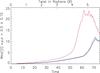 |
Fig. 7 Maximum magnitude of current density in 0.4 <x,y,z< 0.6 for cases (i) 2 sources; (ii) 4 weak sources and (iii) 4 compact sources shown in pink, blue, and black, respectively. |
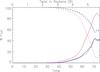 |
Fig. 8 Total percentage of flux connected to sources other than the original source on the upper boundary (solid line) and the percentage of flux connected to its original source (dashed line) for cases (i); (ii) and (iii) shown in pink, blue, and black, respectively. |
The average percentage of flux that remains at its original connection is shown by a dashed line in Fig. 8 for each of the three cases. Initially, 100% of the flux is associated with its original connectivity, but as the current increases, this begins to decrease for all three cases. The percentage of flux associated with a different source (i.e not its original connection) is also plotted (solid line) in pink, blue and black for cases (i), (ii) and (iii), respectively. In these simulations, the absence of any additional background field means that all of the flux is assigned to one of the sources and these values therefore total to 100%.
We note that even though the field is line-tied at the boundaries, due to some numerical slippage taking place, it is not exactly the same field lines that are being considered at each time-step. Instead we describe the proportion of field lines with each connectivity at each time. In addition, the percentage of flux connected to a different source (in Fig. 8) does not necessarily equal the reconnection rate, as the field lines can “slip” while being assigned to the same source. However, it can provide a comparison between the cases and a general indication of the evolution and timing of the change in connectivity in the simulations.
Similarly to the current evolution, there appears to be two stages in the field line connectivity evolution: a gradual increase followed by a sharp increase after t ≈ 50 and t ≈ 60 for the two- and four-source cases, respectively. At these times the magnetic pressure force begins to change direction to act inwards locally around the current layers. This is due to the magnetic field that builds up in the centre of the domain beginning to reconnect and hence the field strength along the current layers reduces. The gradient in B2 creates the inwards magnetic pressure force around the current layer, while further away from the central current layer the magnetic pressure continues to act outwards.
In Fig. 8, the maximum percentage of flux which has changed connectivity in case (i) is 90% and occurs at t = 73, after which the field lines begin to change back to their original connectivity. The evolution of the percentage of flux changing connectivity is comparable for the simulations with four sources, and as with the current evolution, increases later than in the two-source case. Cases (ii) and (iii) reach similar peak values of flux reconnected of 42% and 45% by t = 70 and t = 71, respectively. However, unlike in the two-source case, there are now three possible sources to connect to (other than the original). The percentage of flux at a different connectivity (solid lines in Fig. 8) does not show when field lines that have already changed connectivity undergo multiple reconnection events. In fact, a detailed analysis of the field line connectivity in these cases show multiple reconnections do occur, as suggested by Parnell et al. (2011). The percentages in Fig. 8 are therefore a minimum estimate only. Despite this, we can see in cases (ii) and (iii), a higher percentage of the flux remains at its original connection for the duration of the simulations.
The change in connectivity of the field lines results in strong outflow velocities from the end of the current layers. White arrows showing the projected horizontal velocity components in the central region (0.25 <x,y< 0.75) in the mid-plane are displayed in Fig. 9 for case (i) at t = 60. These show large velocities from the narrow current layer along x = 0.5, where the maximum velocity is ≈0.27vAmax, where vAmax is the maximum Alfvén velocity in the mid-plane (at t = 62.5), an indication of reconnection occurring. We note, that the magnetic field is 3D and reconnection is not confined to the mid-plane, but use the current contours and velocities in the mid-plane to illustrate the differences between the cases.
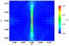 |
Fig. 9 Contour of the magnitude of the current density in the mid-plane between 0.25 <x,y< 0.75 at t = 60 for case (i) with 2 sources. The arrows show the projected velocity in the plane. |
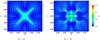 |
Fig. 10 Contours of the magnitude of the current density in the mid-plane between 0.25 <x,y< 0.75 at a) t = 65 and b) t = 70 for case (ii) with 4 weak sources. The arrows show the projected velocity in the plane. |
Similarly, in case (ii), strong outflow velocities are seen from the current “wings” shown in Fig. 10a at t = 65 and very similar behaviour is observed for case (iii) (not shown). Later in cases (ii) and (iii), the current contours in Fig. 10b show the “X” current formation to fragment and then (in addition to the outwards velocity towards the edge of the domain) there are inwards velocity outflows of reconnected field lines towards the centre of the mid-plane. This leads to further current being built up in the centre of the domain. The maximum velocity (in the mid-plane) for cases (ii) and (iii) are 0.05vAmax and 0.04vAmax, respectively, and occurs at t ≈ 74, after this fragmentation of the “X” current formation. This is much smaller than in case (i) and suggests that the reconnection is weaker.
The location of the sources in the case with two flux tubes appears highly idealised to produce the concentrated single current layer in the centre of the domain. In comparison, in the four-source case, as they are evenly distributed around the centre of rotation, a shear is first created between the neighbouring flux tubes, which due to the relative angles of the magnetic field lines will always be less than that induced in the two-source case and produces reduced current values and results in a smaller percentage of flux changing connectivity.
3.1.2. Energetics
The energy evolution is shown by the volume integrated energy densities in Fig. 11 for the cases with two, four weak and four compact sources, displayed in pink, blue and black, respectively and can be described as follows: when the driving velocity acts on the field, the field lines are advected and the magnetic field becomes twisted, gradually increasing the magnetic energy in the domain (see Fig. 11c). Due to the twisted field lines and induced Lorentz force, locations of high current values are created and diffusion becomes important allowing the field lines to reconnect, enabling the built up magnetic energy to be converted into internal energy. As energy is continually added to the domain, the magnetic energy continues to increase, but at a slower rate as the magnetic energy is also being converted into internal and kinetic energy. A sudden increase in kinetic energy occurs from the outflow of the reconnected field lines, shown at different times for the three cases in Fig. 11a.
The magnetic energy in Fig. 11c is the dominating contribution to the total energy evolution. The initial volume integrated magnetic energy density differs between the three cases on the order of 10-4, approximately a 30% variation, due to the construction of the initial flux tubes. Initially, the magnetic energy increases similarly for the three cases as we would expect, until after t ≈ 50 when the magnetic energy does not increase as quickly for case (i) (pink). At this time there is sharp increase of the internal energy for the two-source case (pink) in Fig. 11b, as the magnetic energy is converted to internal energy, faster than in cases (ii) and (iii). This results in a total increase in the internal energy of 56% for case (i) compared to 42% for cases (ii) and (iii).
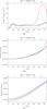 |
Fig. 11 a) Kinetic; b) internal; and c) magnetic volume integrated energies for cases (i); (ii) and (iii) shown in pink, blue, and black respectively. |
For case (i), there is also a larger increase in the kinetic energy at t = 50, tripling the value in 10 time units. This timing coincides with the increase in the percentage of flux changing connectivity, between t = 50 and t = 60 shown in Fig 8, indicating the kinetic energy spike occurs due to the fast outflow of reconnected field lines. In comparison, for cases (ii) and (iii), the rise in kinetic energy occurs later, at approximately t = 60. The kinetic energy also reaches a smaller maximum, of 25% of the peak kinetic energy recorded in case (i). The later increase in the kinetic energy for the four-source cases corresponds to the delay in the increase of the maximum current (and the reconnected field lines) compared to the two-source case.
The total energy being injected into the system over time is given by the Poynting flux:  (11)calculated on the upper and lower boundaries of the domain, as there is no vertical velocity through the z-boundaries and the side boundaries of the domain are closed.
The evolution of the Poynting flux (crosses) is shown in Figs. 12i and ii for cases (i) and (ii), respectively. Case (iii) is not shown as it is the same as for case (ii). Initially the Poynting flux increases very similarly for all three cases, as we would expect, as the three cases have the same total surface magnetic flux and driving velocity. However, as the simulations continue and the magnetic field evolves and reconnects at different times, the subsequent evolution of the Poynting flux varies between the cases.
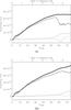 |
Fig. 12 Poynting flux (crosses) with time, for cases (i) 2 sources and (ii) 4 weak sources. The solid line shows the rate of change of magnetic energy, the dotted line work done by the Lorentz force and the dashed line represents the Joule dissipation. |
The Poynting flux into the domain can be divided into the three integrated volume contributions: the rate of change of the magnetic energy, the Ohmic (Joule) dissipation and the work done by the Lorentz force. The evolution of each of these terms is plotted in Fig. 12. Initially, for all three simulations, the bulk of the Poynting flux injected into the domain is seen as the rate of change of the magnetic energy (solid line) as the field becomes highly twisted. As the magnitude of the current density gradually increases in the domain, as seen in Fig. 7, the Joule dissipation (dashed line) builds up slowly in all cases.
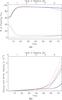 |
Fig. 13 a) Integrated time and volume contributions of the rate of the change of the magnetic energy (solid), the work done by the Lorentz force (dotted) and the Joule dissipation (dashed) as a percentage of the integrated Poynting flux and b) integrated Ohmic (dashed) and viscous (solid) heating, for cases (i); (ii) and (iii) shown in pink, blue, and black, respectively. |
The different current density evolutions in the three cases, produce different evolutions in the Joule dissipation. When the magnitude of the current density increases sharply, which occurs first in case (i) at t = 50, we see a corresponding faster rise in the Joule dissipation in Fig. 12i. Approximately 10 time units later, the Joule dissipation increases in Fig. 12ii for case (ii) (and case (iii), not shown). The Joule dissipation has a maximum value of 1.8 × 10⁻⁵ at t = 65 in case (i) compared to a peak of 1.5 × 10⁻⁵, but at a later time of t = 71, for cases (ii) and (iii).
When the sharp increase in the Joule dissipation occurs, the rate of change of the magnetic energy begins to decrease in all the cases, as the magnetic energy is converted through reconnection into kinetic and internal energy. The rate of change in magnetic energy reduces by approximately 5 × 10⁻⁶ (7%) for both cases (ii) and (iii), before beginning to increase again. In other words, the magnetic energy injected into the system by the continuous driving velocity must be greater than the magnetic energy released through diffusion and reconnection. There is a three times larger decrease in the rate of change in magnetic energy for case (i), of 1.7 × 10⁻⁵ (26%). In case (i), after t = 56 we are unable to fully resolve the current layer and this causes a small loss of energy conservation of approximately 4% of the total Poynting Flux. This loss of energy conservation implies that the change in magnetic energy is reduced through numerical diffusion without the corresponding increase in the Joule dissipation or work done by the Lorentz force. The value of the Joule dissipation in Fig. 12i can therefore be considered as a lower bound for the two-source case.
In these experiments, the Joule dissipation never becomes greater than the rate of change in magnetic energy. In other words, there is always more energy being injected through the boundary driving than being dissipated. This is in contrast to the experiments carried out by De Moortel & Galsgaard (2006a) and Wilmot-Smith & De Moortel (2007), where, for a similar two flux tube experiment, the dissipation exceeded the injected magnetic energy due to the fast reconnection occurring. However, the Joule dissipation and reconnection are strongly dependent on the resistivity used in the simulations.
Due to the reconnection taking place earlier in case (i), compared to cases (ii) and (iii), the magnetic field rearrangement from reconnection results in less Poynting flux being injected into the domain at later times. This is visible in Fig. 12, where, by the end of the experiment, the Poynting flux entering the domain is approximately 7.2 × 10⁻⁵ for case (i), which is 20% less than the Poynting flux entering the domain at t = 75 for cases (ii) and (iii).
It is, therefore, useful to consider the components as a percentage of the integrated Poynting flux over time (see Fig. 13a). For case (i), in pink, by the end of the simulation 10% of the Poynting flux has gone into Joule dissipation (dashed line). However, as discussed, this can be considered a minimum estimate. A slightly smaller value (≈6%), of the Poynting flux goes into Joule dissipation for both of the four-source cases. This suggests that the two-source case is more efficient at Ohmic heating, as we would assume from the higher current values. However, the three cases are generally rather inefficient at converting energy into heating, and the majority of the energy remains in the magnetic field, but these values are highly dependent on the value and form of resistivity used.
3.1.3. Distribution and magnitude of heating
In addition to Ohmic heating (Joule dissipation), the shock viscosity present in our simulations leads to viscous heating. Figure 13b shows the evolution of the volume and time integrated Ohmic heating (dashed) and viscous heating (solid). In all three cases the Ohmic heating is the larger contribution to the total heating. The Ohmic heating also begins to increase before the viscous heating in all three cases, initially increasing gradually and then more rapidly, reflecting the evolution of the maximum current value in Fig. 7. Similarly, the viscous heating appears to evolve in two distinct stages: an initial slow increase followed by a sudden larger increase, due to the high kinetic energies associated with reconnection outflows previously discussed and shown in Fig. 11a. As with the energy and current density evolutions, the increase in the viscous heating appears to occur 10 time units later for the cases with four sources (blue and black). By the end of the simulations, the total viscous heating for the two-source case is 28% larger than both the four-source cases, which are practically identical.
At the time of the most intense Ohmic heating (at t = 60 for case (i) and t = 70 for cases (ii) and (iii)), contours of the square root of the Ohmic heating,  , are displayed in Fig. 14 in the mid-plane (top row) and in the vertical plane y = 0.5 (bottom row). The contours indicate how the Ohmic heating is distributed within the volume.
In the two-source case (i), the Ohmic heating is concentrated along the line x = 0.5 in the mid-plane, where the current layer is formed. In the plane y = 0.5 the heating is similarly confined to the centre of the domain, with the greatest heating occurring towards the mid-plane. However this may be a numeric artefact, due to the resistivity maximum occurring in the mid-plane. In comparison, in the cases (ii) and (iii), with four flux tubes, the Ohmic heating is more spread within the volume, reflecting the larger number of locations with current built up. However, although occurring over a larger area, the values of Ohmic heating in Fig. 14 for cases (ii) and (iii) are much less than for case (i), reflecting the lower current values.
The resultant proportional increase in temperature ((T−Tt = 0) /Tt = 0) from the initial temperature at the start of the simulations (Tt = 0) is displayed in Fig. 15 in the mid-plane (top row) and at y = 0.5 (bottom row) for cases (i), (ii) and (iii) at the same times as shown in Fig. 14. Generally, the temperature increase remains fairly localised towards the central column of the domain, as with the Ohmic heating, with the peak values occurring around the mid-plane. This is as expected as conduction and radiation are not included in the simulations and therefore the temperature increases will be very localised in z and the values will also be higher (than if conduction and radiation were included).
The locations where Ohmic heating is observed clearly show a temperature increase, but the locations of the viscous heating can also be inferred from Fig. 15. Broader more diffuse areas of heating are visible (in light blue) at the end of the current layers, where the reconnection outflows occur and form shocks. Due to the larger number of QSLs in cases (ii) and (iii), there are more locations of reconnection outflows and therefore more locations of viscous heating in Figs. 15ii and iii.
The greatest temperature increase occurs in case (i), in a very small, barely visible region in Fig. 15i. Despite the very similar dynamical evolution of the four-source cases, Fig. 15 also shows a significantly larger temperature increase in the centre of the domain for case (iii) compared to case (ii). This is due to the reduction in density at the centre of the domain from the plasma outflows and therefore a small difference in the amount of heating produces a large variation in the temperature produced.
The maximum increase in the temperatures (as a proportion of the initial temperature Tt = 0) occurring at the centre of the domain is 30.5 (at t = 60), 19.1 and 24.4 (at t = 70) for cases (i), (ii) and (iii), respectively. Using the normalisation value of T0 = 5.76 × 10⁸ K, the illustrative maximum values of temperature are about 6.0 × 10⁷ K, 3.8 × 10⁷ K and 4.8 × 10⁷ K for cases (i), (ii) and (iii), respectively, compared to an initial temperature of 1.9 × 10⁶ K.
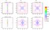 |
Fig. 14 Contours of |
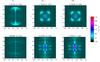 |
Fig. 15 Contours of (T−Tt = 0) /Tt = 0 in the mid-plane (top row) and at y = 0.5 (bottom row) for case (i) at t = 60 and for cases (ii) and (iii) at t = 70. |
These are generally high temperatures, as conduction and radiation effects are not included, and the values are therefore overestimates of the expected increase in temperature from the dissipation described. However, these values are similar to those found by simulations by Bowness et al. (2013) (also without conduction and radiation) when examining the heating produced due to reconnection from shearing a uniform field.
3.2. Two and four source comparisons including a background field
On the solar surface, flux is not distributed as isolated features but as part of a continuous magnetic flux carpet, therefore we now consider the impact of including a background field (BBg) in the experiments. As the two cases with four flux tubes had very similar behaviour in the previous comparison, we shall only consider the case with 4 weak sources (with rsn = 0.065 and Bmaxn = 0.5) and compare it to the 2 source case (Bmaxn = 1.0 and rsn = 0.065). Background field values of BBg = 0.01 and BBg = 0.05 are considered and the prescribed Bz (given by Eq. (7)) on lower boundary is shown in Fig. 16a at y = 0.5, for two (orange) and four (green) flux tube cases with BBg = 0.01 (solid) and BBg = 0.05 (dashed).
The introduction of a background field makes the field lines traced from the sources appear more compact (see Fig. 17) and the strength of the magnetic field in the domain is increased (as shown by the distribution of Bz in the mid-plane in Fig. 16b). The plasma beta value in the domain is therefore reduced, as the density and plasma pressure remain uniform as in the previous comparison.
The same rotational velocity driver is applied to the footpoints of the flux tubes, but an increased maximum resistivity value of η1 = 10-3 is used in Eq. (6) and therefore the corresponding evolution of the two (pink) and four (blue) source cases without background field and with this increased resistivity are presented for comparison. The higher resistivity is used in this comparison as the addition of a background field delays the change in connectivity and for η1 = 10-4 the four-source case shows indications of becoming kink unstable after a large rotation (large θ).
Before continuing with the background field comparison, we first note that increasing the resistivity does not change the qualitative behaviour of the evolutions, but does impact the time-scales and values produced. Although it is not the aim of this paper to investigate the impact of the resistivity on these experiments, we highlight to the reader some general consequences of increasing the resistivity for the simulations with BBg = 0. These include: reduced maximum current and broader current layers; the field line connectivity changing at earlier times (earlier θ), a greater amount (and efficiency) of Ohmic heating and therefore higher temperatures produced; and (due to the higher temperatures and subsequent gas pressure force) the current layer in the two-source cases fragmenting towards the end of the simulations.
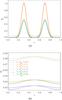 |
Fig. 16 Bz at y = 0.5a) on the lower boundary and b) in the mid-plane for non-background field cases with 2 (pink) and 4 (blue) sources and for cases with BBg = 0.01 (solid) and BBg = 0.05 (dashed) for two and four sources displayed in orange and green, respectively. |
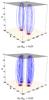 |
Fig. 17 A selection of field lines traced after relaxation from z = 0.0 for cases with a) 2 sources and b) 4 sources with BBg = 0.05. |
The addition of a background field was considered by De Moortel & Galsgaard (2006a) for a two flux tube configuration undergoing rotation. Their results found that the introduction of an additional background flux between the sources on the boundary delayed the flux associated with the sources changing connectivity and produced higher current values and more efficient Joule dissipation. The same qualitative trends are found in our experiments, but we consider whether the impact of the background field is more, less or the same, for a different (four source) flux distribution.
For the cases with background field, the same qualitative description given in Sect. 3.1 of the field evolution and subsequent forces and energetics applies. The current density distributions are therefore also very similar to that shown in Figs. 9 and 10 for the non-background field cases, but the current increases at earlier times due to the increased resistivity. The gradual increase in current, that occurs in all the cases, is shown to increase faster for higher values of background field (see Fig. 18) and the subsequent sharp increase in the current is also steeper.
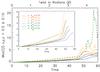 |
Fig. 18 Maximum magnitude of the current density in 0.4 <x,y,z< 0.6 for non-background field cases with 2 (pink) and 4 (blue) sources and for cases with BBg = 0.01 (solid) and BBg = 0.05 (dashed) for two and four sources displayed in orange and green, respectively. |
The inset graph in Fig. 18 shows the initial evolution of max(| j |) until the first maxima of each case. Until this time, the two- and four-source cases follow the same pattern described in the previous comparison, where the increase in current occurs earlier and reaches higher values for the two-source case. However, after these initial maxima, it is the four-source case with BBg = 0.05 (green, dashed line) that is shown to reach the highest values of current density, unlike for the smaller values of background field. In comparison, the two-source case with BBg = 0.05 (yellow, dashed) does not continue to increase at the rate it does before t = 50. Examination of the current in the domain, shows that at this time the single current layer of the two-source case with BBg = 0.05 begins to break up into separate parts, shown in the contour of | j | in Fig. 19a. This occurs due to the initial high current formed in the centre of the current layer producing a localised extremely large temperature increase, which creates an outward pressure force acting against the inwards Lorentz force in the x-direction at y = 0.5. The current values reached in the simulation therefore do not increase as we would expect if the current were continually able to be built up towards the centre of the domain. Instead, the inwards Lorentz force is diverted and forms two current maxima around the centre of the x−y plane. This current layer breakup occurs at all heights in the domain, as shown by the current isosurface in Fig. 19b. The current layer fragmentation also occurs in the two-source case with BBg = 0.01 and BBg = 0.0, but not until after the time shown (t> 60), as in these cases the high temperatures occur later.
The percentage of flux (traced from the sources on z = 0) that has changed connectivity to a different source on the upper boundary (as discussed for Fig. 8) is plotted in Fig. 20a. For non-zero background field values, Fig. 20a shows that there is a delay in the flux associated with sources (on the base) changing connectivity to another source. This delay also increases with the strength of the background field. In particular the two-source case with BBg = 0.05 (yellow, dashed line) does not have any flux associated with a different source until t = 38, a delay of 22 time units from the case with BBg = 0 (pink). In contrast, the four-source case with BBg = 0.05 (green, dashed line) has a comparatively short delay, of only 10 time units.
However, the connectivity diagnostic in Fig. 20a does not account for the flux that is changing connectivity but not associated with another source on the upper boundary. The addition of a background flux means that the field lines associated with sources are able to reconnect continuously across the upper and lower boundaries and therefore large proportions of the flux may be connected to the background field. Figure 20b displays the percentage of flux (traced from the lower boundary sources) that is connected to its original source on the upper boundary, and shows the gradual reduction as the field lines reconnect to both the other sources and the background field. There is also a delay in the flux changing connectivity from its original source for cases with a background field, seen in Fig. 20b, however this is only of the order of ≈5 time units, although it is again slightly greater in the two-source case. This delay is due to confining effect of the background field. The flux associated with the background field needs to first reconnect to be removed and allow the flux tubes to interact.
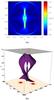 |
Fig. 19 a) Contour and b) isosurface of magnitude 2.0, of the current density for the two flux tube case with BBg = 0.05 at t = 50. |
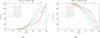 |
Fig. 20 Total percentage of flux a) connected to sources other than the original source on upper boundary and b) connected to the original source, for non-background field cases with two (pink) and four (blue) sources and for cases with BBg = 0.01 (solid) and BBg = 0.05 (dashed) for two and four sources displayed in orange and green, respectively. |
In the cases without background field (pink and blue) the combined flux percentages in Figs. 20a and b account for approximately 100% of the flux from the sources. In contrast, in the cases with background field, where it is easier for the flux to be connected elsewhere on the boundary, there is a percentage of flux that is no longer associated to a source on the boundary (i.e. “unassigned” flux), but has therefore changed its connectivity. This is particularly evident in the two flux tube case with BBg = 0.05 (orange, dashed line). In the four-source cases less flux is considered to be unassigned, however, this may simply be due to the fact that a greater proportion of the boundary is considered to be a “source” compared to the two-source cases.
Despite the delay in the flux associated with the sources changing connectivity, once it has begun, the change in connectivity occurs more rapidly for cases with stronger background magnetic field, shown by the increasing gradients in Fig. 20b. This results in 100% of the flux from the sources on the base reconnecting in the cases with background field, as shown by the reduction of the green and yellow lines to 0 in Fig. 20b. In comparison, in the two- and four-source cases without background field (pink and blue) some flux always remains connected to its original source. The increased rate of change in connectivity is particularly evident in the four-source case with BBg = 0.05 (green, dashed line), reaching a minimum in Fig. 20b before all the other cases. There is a large contrast between the steep change in connectivity of this four-source case with BBg = 0.05 and the four-source case with no background field. In comparison, the increased rate of connectivity is less evident for the two-source case, where the change in connectivity for BBg = 0 was already very fast.
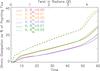 |
Fig. 21 Volume and time integrated Ohmic dissipation, shown as a percentage of the time integrated Poynting flux, for non-background field cases with two (pink) and four (blue) sources and for cases with BBg = 0.01 (solid) and BBg = 0.05 (dashed) for two and four sources displayed in orange and green, respectively. |
Due to the increased magnetic field on the boundaries, a larger amount of energy is entering the domain for each of the cases with a background field. We therefore consider the time and volume integrated Ohmic dissipation as a percentage of the integrated Poynting flux (see Fig. 21), to compare the efficiency of the heating between the cases. Similar to the findings of De Moortel & Galsgaard (2006a), the higher current values and faster change in connectivity associated with the cases with background field, produces greater efficiency of Ohmic heating. For all values of background field, the two and the four-source cases behave similarly to begin with and then the four-source cases begin to show a larger increase in the Ohmic heating than the two source counterpart. The percentages of Ohmic heating at t = 60 (or θ = 4.5 rad) are 20%, 26% and 37% for the two-source cases with increasing background field values (of Bbg = 0, 0.01, 0.05, respectively), compared to 17.5%, 25% and 36.5% for the four-source cases. These values illustrate that the introduction of a background field appears to make the heating produced by the two- and four-source cases more comparable.
3.3. Small-scale sources
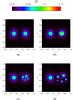 |
Fig. 22 Contour plots of | B | after relaxation at z = 0.0 for cases a) to d) (see text). |
In this section a final comparison to consider the impact of the number of magnetic sources (and their locations) is presented. The original two-source case is extended, by fragmenting one of the sources into 6 smaller sources of various radii. These fragmented sources are all centred around the same location, namely (x,y) = (0,7,0.5). The fragmented source distributions are also described by a summation of Gaussians (see Eq. (7)) on the upper and lower boundary. Three cases are considered with increasingly spread sources, as shown on the lower boundary in Figs. 22b−d, which shall be referred to as cases (b)−(d). For these cases we use BBg = 0.01 and compare them to the two-source case with BBg = 0.01 introduced in the previous section (see Fig. 22a), which we shall refer to as case (a).
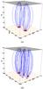 |
Fig. 23 A selection of field lines traced after relaxation from z = 0.0 for cases with a) 2 sources and d) fragmented sources with the largest spread. |
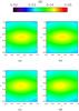 |
Fig. 24 Contour plots of | B | after relaxation in the mid-plane for cases a) to d) (see text). |
The flux tubes are formed from this vertical flux distribution as described in Sect. 2.2 and displayed for cases (a) and (d) in Fig. 23. The resultant field strength in the mid-plane, shown in Fig. 24, is very similar for all the cases, as the magnetic field expands from the boundary to form a fairly uniform magnetic field in the mid-plane. It is only in the case with the largest spread of fragmented sources that the field strength appears slightly altered, with the maximum occurring off the centre of the plane. This asymmetry is introduced due to a slight imbalance in the amount of flux either side of the line y = 0.5, as, in this case, the flux sources are spread over the widest area.
These initial magnetic field configurations are evolved using the same velocity driver and with the resistivity value of η1 = 10-3, as used in the background field comparisons. The velocity driver acts to twist the magnetic field and the evolution of the maximum current with time for the fragmented cases (shown in green, blue and black for cases (b)−(d)) increases gradually at first and then more steeply, with a very similar evolution to the two-source case (a), shown in pink in Fig. 25. At t ≈ 52 the | jmax | forms an initial maximum and there is minimal difference between the cases, with the highest value of 4.8 (recorded in section 0.4 <x,y,z< 0.6) occurring for the largest spread fragments case (black) and the smallest value of | jmax | of 4.4 at this time occurs for the least spread fragments case (green).
The distribution of the current is shown in the mid-plane for the cases (just before the initial maxima) at t = 50 in Fig. 26. The high current is formed along the line y = 0.5 in the mid-plane and extends with height in the form of a twisted current sheet for all the cases, as described in detail for the two-source case in Sect. 3.1. In contrast to the change in the current formation produced by the two- and four-source comparison, the current concentrations are almost identical between the cases with the fragmented sources and the two-source case. The one exception is the slightly warped current layer that is formed in the case with the largest spread of flux fragments in Fig. 26d. This is due to the initial flux imbalance that was seen in the mid-plane in Fig. 24d, which leads to a stronger Lorentz force on one side of the domain. Despite the fragmented source structure on the z-boundaries, the applied large-scale rotation acts to move the sources as one and therefore the gradients in the magnetic field that are formed are largely comparable to the two-source case.
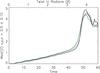 |
Fig. 25 Maximum magnitude of the current density between 0.4 <x,y,z< 0.6 for cases a) to d) in pink, green, blue and black, respectively. |
The twisted magnetic field is shown in 3D for the two-source case and the largest spread fragmented source case (d) in Fig. 27 at t = 50 (after a rotation of θ = 3.8 rad ≈1.2π). The field lines are traced from the same locations around the central current layer in the mid-plane in both cases (the colours represent values of E||, where red is high and blue is low E||). The general shape of the twisted field lines is very similar between the cases for the majority of the domain. It is only very close to the upper and lower boundaries that the field lines in Fig. 27d diverge to the separate fragments.
After t = 52, the maximum current (see Fig. 25) begins to decrease slightly as the magnetic field is able to diffuse. The evolution then becomes more erratic and there is some variability seen between the cases. This is due to the break up of the single current layer into smaller distributed current concentrations, as previously discussed for the two-source case with background field.
The comparable field evolution and current formation in the domain imply that a similar amount of heating due to Ohmic dissipation will also occur. This is supported by Fig. 28, which shows the integrated Ohmic dissipation as a percentage of the integrated Poynting flux into the domain and indicates that the efficiency of heating is very similar for all the cases with a maximum variation of 1.5% by the end of the simulation.
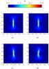 |
Fig. 26 Contour plots of the magnitude of the current density in the mid-plane at t = 50 for cases a) to d) (see text). |
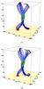 |
Fig. 27 Field lines traced from the centre of the mid-plane at t = 50 and coloured by the value of E|| for cases a) and d). |
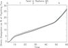 |
Fig. 28 Time and volume integrated Ohmic heating as a percentage of the integrated Poynting flux at each time, for cases a) to d). |
4. Discussion and conclusions
In this paper we have considered a series of experiments with different flux distributions (producing different flux tube configurations) undergoing the same driving on the boundaries. Maintaining the same total flux and the same velocity enables us to isolate the impact of the flux distribution on the current formation and heating.
The initial comparison was between a case with two flux tubes and two cases with four flux tubes, with different radii and strength but the same total magnetic flux. However, we note that the four-source cases behaved (almost) identically and when we refer to the “four-source case” we shall therefore be referring to both. The comparison shows that redistributing the flux from “two sources” to “four sources” (for our chosen source distribution and velocity driver) reduces the build up of current in the domain. The maximum current reached for the four-source case is half the value produced for the two-source case and, due to the increased number of regions of different connectivity to begin with, there are more locations (QSLs) where the current is seen to build up.
The larger area of current but with reduced peak values results in a delay in the onset of reconnection in the four-source case. The reconnection that occurs is also shown to be less energetic with reduced outflows. However, the increased number of sources in the four flux tube case, does increase the possible connectivities and enables further current concentrations to build up later in the simulations, due to the further interaction of the outflows of the reconnected field.
The Ohmic heating accounts for 6% of the Poynting flux entering the domain, compared to 10% for the two-source case. These heating values are relatively low, as in this comparison a large proportion (83% and 89% for two- and four-source cases) of the energy input into the domain remains stored in the highly twisted magnetic field. These values are of course highly dependent on resistivity.
The impact of including a background field between the flux sources is also investigated for a two and a four flux tube case, with a higher value of resistivity used. The introduction of a background field increases the field strength in the domain and the current increases to higher values, although the locations of current formation are similar to the non-background field case. Despite the higher current values, the background field between the flux tubes delays the flux associated with the sources from reconnecting, but when it does reconnect the change in connectivity is shown to occur faster for cases with stronger background field, for both the two- and four-source cases. However, there is also some evidence that the impact of the background field is more apparent for the cases with four flux tubes, which had a slower change in the connectivity in the non-background field cases. The two- and four-source cases therefore appear more comparable when there are greater values of background field between them.
The increased resistivity value in these comparisons resulted in larger proportions of the energy entering the domain being converted to Ohmic heating, between 20% and 40% for cases with different background field values, and at earlier times and therefore after smaller rotation angles.
In our experiments the results are discussed in terms of normalised values as we are chiefly concerned with the comparison between the cases. However, using the suggested normalisation values outlined in Sect. 2.1, the total dissipated energy values in a coronal context for the background field comparison are between (3−9) × 1029 erg, for cases with 0−5% background field, where the cases with a background field have more energy entering the domain. These are very high dissipation energies, but the values clearly depend on the normalisation and initial conditions chosen: for example the size of the flux tubes considered (with sources of radius 4.8 Mm) are very large compared to the small scale of the coronal loops strands observed, and which are assumed to be associated with the predicted small-scale nanoflare heating events. The heating values produced may therefore be scaled down when considering smaller magnetic features. Similarly, we note that the values of heating produced will be highly dependent on the parameter values chosen: for example for resistivity and shock viscosity.
A final comparison, with a series of smaller fragmented sources, which were positioned around the same location as one of the sources in the two flux tube case, is considered. However, the positioning and relative scale of the fragments meant the large-scale driver acts on the fragments to move them as one. Subsequently, there was little interaction (or current formed) between the flux fragments and the general field evolution was qualitatively and quantitatively similar to the two-source case. This implies that the evolution of the magnetic field and therefore the current formation cannot be interpreted in terms of the complexity of the magnetic flux distribution alone, but must be considered relative to the scale and location of the velocity driver.
In future investigations drivers of different scales could be considered, as well as alternative forms of velocity drivers such as shears and more complex random motions. These would enable the flux fragments to move independently and may therefore alter the evolution and subsequent heating in the fragmented source comparisons.
The experiments described here are very idealised and there are many avenues for possible future work. In addition to the possibility of considering different velocity drivers, we could also consider different applications of resistivity. In these experiments a localised resistivity (centred on the mid-plane and reducing towards the footpoints) is used in order to prevent the isolated flux structures on the boundaries from diffusing. However, in reality reconnection and heating is expected to occur at lower heights towards the footpoints of the loops as well.
Similarly, the resistivity values of 10-4 and 10-3 may be viewed as high. In the corona the resistivity is generally expected to be extremely low, of the order of 10-6 Ω m, producing a high magnetic Reynold’s number (Rm) and therefore the magnetic field will largely evolve without diffusion. In current sheets, where the magnetic field changes over small length-scales (Rm reduces), the magnetic energy is able to dissipate. However, in numerical simulations there is always an associated numerical diffusion term that acts to diffuse the magnetic energy in locations of high current formation. Therefore when examining the evolution of energy it is important to chose a large enough resistivity in order to accurately follow the conversion of energy from being stored in the magnetic field into kinetic and internal energy (Bowness et al. 2013), without significant numerical diffusion. Any significant loss in energy conservation would prevent an accurate comparison between the different cases, as each would be dependent on the unknown and variable numerical diffusivity. The resistivity is present for the entire simulation and we suspect that if smaller values of resistivity were able to be used (at higher resolutions) a smaller percentage of the energy input into the domain would we dissipated due to the gradual Ohmic dissipation that occurs for the majority of the simulations.
However, if an anomalous resistivity was used and therefore the resistivity was not present from the start of the simulations but applied at specific locations when high current values are formed, then initially less heating would occur and a larger amount of Poynting flux would enter the domain. This would also result in higher currents values being produced and suggests that when reconnection does occur it would be more energetic and efficient. This implies that, with an anomalous resistivity, a greater difference in the current values, as is the case in the two- and four-source comparison, may create a greater variation in the heating produced than our results imply.
In all the experiments, the Ohmic heating is shown to dominate the viscous heating. This is due to the absence of any constant physical viscosity (ν) and the viscous heating is due solely to the shock viscosity in Lare3D. In reality in the corona ν ≫ η and viscosity is expected to play an important role in heating the plasma. Indeed, many numerical investigations (e.g. Armstrong & Craig 2014) have shown that viscous dissipation should dominate resistive dissipation and account for a large fraction of energy release in flares.
We also note that the velocity driver applies significant rotation to the flux tubes of up to θ = 5.7 rad (in the first comparison) on one boundary and therefore a total twist of 2θ = 11.4 rad ≈3.6π. These may be considered large amounts of continual twist, greater than observed velocity motions on the solar surface (e.g. by Bonet et al. 2008). However, in reality the flux tubes being advected in the solar atmosphere will not be in a near potential state initially and therefore less rotation would be needed to create current concentrations.
The simplified atmosphere modelled in our experiments has an initial uniform density and pressure, which results in plasma beta values higher than predicted in the solar corona, particularly in the mid-plane where the field strength is weakest. Future experiments using a stratified atmosphere may also be considered, where a resultant reduction in the plasma beta may also impact the plasma evolution, reconnection and subsequent heating (Birn et al. 2009; Galsgaard 2002). Similarly, in our models thermal conduction and radiation are neglected and therefore very high (>108 K) temperatures were produced, as the heating was not able to be distributed. However, Botha et al. (2011) showed that high localized temperatures were reduced by a factor of 10 when thermal conduction is included.
Our simulations examine the impact of the distribution of flux in these “elementary” flux tube interactions and the associated heating. However, despite their simplicity, these simulations can, in turn, help our understanding of the general behaviour of larger and more complex models, where the resolution does not allow for the small-scale energy events to be analysed in detail. Our results also lead to many further questions and possibilities to explore, from reducing the symmetry and regularity of the flux tube distribution, to varying the form and scale of the velocity driver. In the future, models could gradually increase the complexity of these elementary heating events in these ways, in order to fully understand the impact of each contribution.
Acknowledgments
This work used the COSMA Data Centric system at Durham University, operated by the Institute for Computational Cosmology on behalf of the STFC DiRAC HPC Facility (www.dirac.ac.uk). This equipment was funded by a BIS National E-infrastructure capital grant ST/K00042X/1, STFC capital grant ST/K00087X/1, DiRAC Operations grant ST/K003267/1 and Durham University. DiRAC is part of the National E-Infrastructure. I.D.M. was funded by the Science and Technology Facilities Council (UK). The research leading to these results has also received funding from the European Research Council (ERC) under the European Union Horizon 2020 research and innovation programme (grant agreement No. 647214). J.P.O was funded by the Science and Technology Facilities Council (UK) by Doctoral Grant ST/K502327/1.
References
- Arber, T. D., Longbottom, A. W., Gerrard, C. L., & Milne, A. M. 2001, J. Comput. Phys., 171, 151 [NASA ADS] [CrossRef] [Google Scholar]
- Armstrong, C. K., & Craig, I. J. D. 2014, Sol. Phys., 289, 869 [NASA ADS] [CrossRef] [Google Scholar]
- Aulanier, G., Pariat, E., Démoulin, P., & DeVore, C. R. 2006, Sol. Phys., 238, 347 [NASA ADS] [CrossRef] [Google Scholar]
- Ballegooijen, A. A. V. 1988, Geophys. Astrophys. Fluid Dyn., 41, 181 [NASA ADS] [CrossRef] [Google Scholar]
- Baumann, G., Galsgaard, K., & Nordlund, Å. 2013, Sol. Phys., 284, 467 [NASA ADS] [CrossRef] [Google Scholar]
- Birn, J., Fletcher, L., Hesse, M., & Neukirch, T. 2009, ApJ, 695, 1151 [NASA ADS] [CrossRef] [Google Scholar]
- Bonet, J. A., Márquez, I., Sánchez Almeida, J., Cabello, I., & Domingo, V. 2008, ApJ, 687, L131 [NASA ADS] [CrossRef] [Google Scholar]
- Botha, G. J. J., Arber, T. D., & Hood, A. W. 2011, A&A, 525, A96 [NASA ADS] [CrossRef] [EDP Sciences] [Google Scholar]
- Bowness, R., Hood, A. W., & Parnell, C. E. 2013, A&A, 560, A89 [NASA ADS] [CrossRef] [EDP Sciences] [Google Scholar]
- Brooks, D. H., Warren, H. P., Ugarte-Urra, I., & Winebarger, A. R. 2013, ApJ, 772, L19 [NASA ADS] [CrossRef] [Google Scholar]
- De Moortel, I., & Galsgaard, K. 2006a, A&A, 451, 1101 [NASA ADS] [CrossRef] [EDP Sciences] [Google Scholar]
- De Moortel, I., & Galsgaard, K. 2006b, A&A, 459, 627 [NASA ADS] [CrossRef] [EDP Sciences] [Google Scholar]
- Démoulin, P., Henoux, J. C., Priest, E. R., & Mandrini, C. H. 1996a, A&A, 308, 643 [NASA ADS] [Google Scholar]
- Démoulin, P., Priest, E. R., & Lonie, D. P. 1996b, J. Geophys. Res., 101, 7631 [NASA ADS] [CrossRef] [Google Scholar]
- Galsgaard, K. 2002, in SOLMAG 2002, in Proc. of the Magnetic Coupling of the Solar Atmosphere Euroconference, ed. H. Sawaya-Lacoste, ESA SP, 505, 269 [Google Scholar]
- Galsgaard, K., & Nordlund, Å. 1996, J. Geophys. Res., 101, 13445 [NASA ADS] [CrossRef] [Google Scholar]
- Janvier, M., Aulanier, G., & Démoulin, P. 2015, Sol. Phys., 290, 3425 [NASA ADS] [CrossRef] [Google Scholar]
- Lau, Y.-T., & Finn, J. M. 1990, ApJ, 350, 672 [NASA ADS] [CrossRef] [Google Scholar]
- Longcope, D. W., & Sudan, R. N. 1994, ApJ, 437, 491 [NASA ADS] [CrossRef] [Google Scholar]
- Mellor, C., Gerrard, C. L., Galsgaard, K., Hood, A. W., & Priest, E. R. 2005, Sol. Phys., 227, 39 [NASA ADS] [CrossRef] [Google Scholar]
- Ng, C. S., Lin, L., & Bhattacharjee, A. 2012, ApJ, 747, 109 [NASA ADS] [CrossRef] [Google Scholar]
- Parker, E. N. 1972, ApJ, 174, 499 [NASA ADS] [CrossRef] [Google Scholar]
- Parker, E. N. 1979, Cosmical magnetic fields: Their origin and their activity (Oxford University Press) [Google Scholar]
- Parker, E. N. 1988, ApJ, 330, 474 [Google Scholar]
- Parker, E. N. 1994, Spontaneous current sheets in magnetic fields: with applications to stellar X-rays, Int. Ser. Astron. Astrophys. (New York: Oxford University Press), Vol. 1 [Google Scholar]
- Parnell, C. E., Haynes, A. L., & Galsgaard, K. 2010, J. Geophys. Res. (Space Physics), 115, 2102 [Google Scholar]
- Parnell, C. E., Maclean, R. C., Haynes, A. L., & Galsgaard, K. 2011, in IAU Symp. 271, eds. N. H. Brummell, A. S. Brun, M. S. Miesch, & Y. Ponty, 227 [Google Scholar]
- Parnell, C. E., Stevenson, J. E. H., Threlfall, J., & Edwards, S. J. 2015, Philosoph. Trans. R. Soc. Lond. Ser. A, 373, 20140264 [Google Scholar]
- Pontin, D. I., Galsgaard, K., Hornig, G., & Priest, E. R. 2005, Phys. Plasmas, 12, 052307 [NASA ADS] [CrossRef] [Google Scholar]
- Priest, E. R., & Démoulin, P. 1995, J. Geophys. Res., 100, 23443 [NASA ADS] [CrossRef] [Google Scholar]
- Priest, E. R., Heyvaerts, J. F., & Title, A. M. 2002, ApJ, 576, 533 [NASA ADS] [CrossRef] [Google Scholar]
- Priest, E. R., Hornig, G., & Pontin, D. I. 2003, J. Geophys. Res., 108, 1285 [Google Scholar]
- Rappazzo, A. F., Velli, M., Einaudi, G., & Dahlburg, R. B. 2007, ApJ, 657, L47 [NASA ADS] [CrossRef] [Google Scholar]
- Rappazzo, A. F., Velli, M., Einaudi, G., & Dahlburg, R. B. 2008, ApJ, 677, 1348 [NASA ADS] [CrossRef] [Google Scholar]
- Scullion, E., Rouppe van der Voort, L., Wedemeyer, S., & Antolin, P. 2014, ApJ, 797, 36 [NASA ADS] [CrossRef] [Google Scholar]
- Stevenson, J. E. H., Parnell, C. E., Priest, E. R., & Haynes, A. L. 2015, A&A, 573, A44 [NASA ADS] [CrossRef] [EDP Sciences] [Google Scholar]
- Title, A. M., & Schrijver, C. J. 1998, in Cool Stars, Stellar Systems, and the Sun, eds. R. A. Donahue, & J. A. Bookbinder, ASP Conf. Ser., 154, 345 [Google Scholar]
- Wilmot-Smith, A. L. 2015, Phil. Trans. R. Soc. Lond. Ser. A, 373, 20140265 [Google Scholar]
- Wilmot-Smith, A. L., & De Moortel, I. 2007, A&A, 473, 615 [NASA ADS] [CrossRef] [EDP Sciences] [Google Scholar]
All Figures
|
Fig. 1 Profile of the imposed driving velocity (black) and profile of Bz (red) and | B | (blue) for the two-source case (i) at z = 0.0 and y = 0.5. |
| In the text | |
|
Fig. 2 Magnetic source labels at t = 0 on a) z = 0.0 and b) z = 1.0. The direction of rotation is also indicated. |
| In the text | |
|
Fig. 3 Contour plots of | B | after relaxation at z = 0.0 (left column) and z = 0.5 (right column) for cases with (i) 2 sources (top row); (ii) “weak” 4 sources (middle row) and (iii) “compact” 4 sources (bottom row). |
| In the text | |
|
Fig. 4 A selection of field lines traced from z = 0.0 for cases i) 2 sources; ii) 4 sources (weak); and iii) 4 sources (compact). |
| In the text | |
|
Fig. 5 Projected Lorentz force in the plane (arrows) over-plotted on contours of the magnitude of the current density in the mid-plane between 0.25 <x,y< 0.75 at t = 50 for case i) 2 sources; and at t = 60 for cases ii) 4 weak sources and iii) 4 compact sources. |
| In the text | |
|
Fig. 6 A selection of field lines traced from source C on z = 0 at t = 60 for cases i) 2 sources; ii) 4 weak sources and iii) 4 compact sources, coloured according to their connectivity. Over-plotted are the isosurfaces of the current density of magnitude 2.5 within the central box (0.1 <x,y,z< 0.9) in the domain. |
| In the text | |
|
Fig. 7 Maximum magnitude of current density in 0.4 <x,y,z< 0.6 for cases (i) 2 sources; (ii) 4 weak sources and (iii) 4 compact sources shown in pink, blue, and black, respectively. |
| In the text | |
|
Fig. 8 Total percentage of flux connected to sources other than the original source on the upper boundary (solid line) and the percentage of flux connected to its original source (dashed line) for cases (i); (ii) and (iii) shown in pink, blue, and black, respectively. |
| In the text | |
|
Fig. 9 Contour of the magnitude of the current density in the mid-plane between 0.25 <x,y< 0.75 at t = 60 for case (i) with 2 sources. The arrows show the projected velocity in the plane. |
| In the text | |
|
Fig. 10 Contours of the magnitude of the current density in the mid-plane between 0.25 <x,y< 0.75 at a) t = 65 and b) t = 70 for case (ii) with 4 weak sources. The arrows show the projected velocity in the plane. |
| In the text | |
|
Fig. 11 a) Kinetic; b) internal; and c) magnetic volume integrated energies for cases (i); (ii) and (iii) shown in pink, blue, and black respectively. |
| In the text | |
|
Fig. 12 Poynting flux (crosses) with time, for cases (i) 2 sources and (ii) 4 weak sources. The solid line shows the rate of change of magnetic energy, the dotted line work done by the Lorentz force and the dashed line represents the Joule dissipation. |
| In the text | |
|
Fig. 13 a) Integrated time and volume contributions of the rate of the change of the magnetic energy (solid), the work done by the Lorentz force (dotted) and the Joule dissipation (dashed) as a percentage of the integrated Poynting flux and b) integrated Ohmic (dashed) and viscous (solid) heating, for cases (i); (ii) and (iii) shown in pink, blue, and black, respectively. |
| In the text | |
|
Fig. 14 Contours of |
| In the text | |
|
Fig. 15 Contours of (T−Tt = 0) /Tt = 0 in the mid-plane (top row) and at y = 0.5 (bottom row) for case (i) at t = 60 and for cases (ii) and (iii) at t = 70. |
| In the text | |
|
Fig. 16 Bz at y = 0.5a) on the lower boundary and b) in the mid-plane for non-background field cases with 2 (pink) and 4 (blue) sources and for cases with BBg = 0.01 (solid) and BBg = 0.05 (dashed) for two and four sources displayed in orange and green, respectively. |
| In the text | |
|
Fig. 17 A selection of field lines traced after relaxation from z = 0.0 for cases with a) 2 sources and b) 4 sources with BBg = 0.05. |
| In the text | |
|
Fig. 18 Maximum magnitude of the current density in 0.4 <x,y,z< 0.6 for non-background field cases with 2 (pink) and 4 (blue) sources and for cases with BBg = 0.01 (solid) and BBg = 0.05 (dashed) for two and four sources displayed in orange and green, respectively. |
| In the text | |
|
Fig. 19 a) Contour and b) isosurface of magnitude 2.0, of the current density for the two flux tube case with BBg = 0.05 at t = 50. |
| In the text | |
|
Fig. 20 Total percentage of flux a) connected to sources other than the original source on upper boundary and b) connected to the original source, for non-background field cases with two (pink) and four (blue) sources and for cases with BBg = 0.01 (solid) and BBg = 0.05 (dashed) for two and four sources displayed in orange and green, respectively. |
| In the text | |
|
Fig. 21 Volume and time integrated Ohmic dissipation, shown as a percentage of the time integrated Poynting flux, for non-background field cases with two (pink) and four (blue) sources and for cases with BBg = 0.01 (solid) and BBg = 0.05 (dashed) for two and four sources displayed in orange and green, respectively. |
| In the text | |
|
Fig. 22 Contour plots of | B | after relaxation at z = 0.0 for cases a) to d) (see text). |
| In the text | |
|
Fig. 23 A selection of field lines traced after relaxation from z = 0.0 for cases with a) 2 sources and d) fragmented sources with the largest spread. |
| In the text | |
|
Fig. 24 Contour plots of | B | after relaxation in the mid-plane for cases a) to d) (see text). |
| In the text | |
|
Fig. 25 Maximum magnitude of the current density between 0.4 <x,y,z< 0.6 for cases a) to d) in pink, green, blue and black, respectively. |
| In the text | |
|
Fig. 26 Contour plots of the magnitude of the current density in the mid-plane at t = 50 for cases a) to d) (see text). |
| In the text | |
|
Fig. 27 Field lines traced from the centre of the mid-plane at t = 50 and coloured by the value of E|| for cases a) and d). |
| In the text | |
|
Fig. 28 Time and volume integrated Ohmic heating as a percentage of the integrated Poynting flux at each time, for cases a) to d). |
| In the text | |
Current usage metrics show cumulative count of Article Views (full-text article views including HTML views, PDF and ePub downloads, according to the available data) and Abstracts Views on Vision4Press platform.
Data correspond to usage on the plateform after 2015. The current usage metrics is available 48-96 hours after online publication and is updated daily on week days.
Initial download of the metrics may take a while.