| Issue |
A&A
Volume 593, September 2016
|
|
|---|---|---|
| Article Number | A82 | |
| Number of page(s) | 10 | |
| Section | Galactic structure, stellar clusters and populations | |
| DOI | https://doi.org/10.1051/0004-6361/201628816 | |
| Published online | 27 September 2016 | |
Hiding its age: the case for a younger bulge
1 GEPI, Observatoire de Paris, CNRS, Université Paris Diderot, 5 place Jules Janssen, 92190 Meudon, France
e-mail: Misha.Haywood@obspm.fr
2 School of Physics, Korea Institute for Advanced Study, 85 Hoegiro, Dongdaemun-gu, 02455 Seoul, Republic of Korea
3 National Optical Astronomy Observatorie/AURA, Tucson, AZ 85719, USA
Received: 29 April 2016
Accepted: 8 June 2016
The determination of the age of the bulge has led to two contradictory results. On the one side, the color–magnitude diagrams in different bulge fields seem to indicate a uniformly old (>10 Gyr) population. On the other side, individual ages derived from dwarfs observed through microlensing events seem to indicate a wide spread, from ~2 to ~13 Gyr. Because the bulge is now recognised as being mainly a boxy peanut-shaped bar, it is suggested that disk stars are one of its main constituents, and therefore also stars with ages significantly younger than 10 Gyr. Other arguments also point out that the bulge cannot be exclusively old, and in particular cannot be a burst population, as is usually expected if the bulge were the fossil remnant of a merger phase in the early Galaxy. In the present study, we show that given the range of metallicities observed in the bulge, a uniformly old population would be reflected in a significant spread in color at the turn-off, which is not observed. We demonstrate that the correlation between age and metallicity expected to hold for the inner disk would instead conspire to form a color–magnitude diagram with a remarkably narrow spread in color, thus mimicking the color–magnitude diagram of a uniformly old population. If stars younger than 10 Gyr are part of the bulge, as must be the case if the bulge has been mainly formed through dynamical instabilities in the disk, then a very narrow spread at the turn-off is expected, as seen in the observations.
Key words: Galaxy: abundances / Galaxy: disk / Galaxy: evolution / galaxies: evolution
© ESO, 2016
1. Introduction
Progress in the study of galactic bulges in the past decade has established two different types of bulges: classical and pseudo-bulges (Kormendy & Kennicutt 2004). Classical bulges have properties identical to elliptical galaxies, while pseudo-bulges have properties inherited from the disk from which they are assumed to have formed: they are more flattened, have bluer colors, and rotate faster. In the local volume (distance <11 Mpc), pseudo-bulges are the majority, and classical bulges are few (Kormendy et al. 2010; Fisher & Drory 2010), while some galaxies are known to harbor both types of bulges (Erwin et al. 2015; Fisher & Drory 2016). It has been found first from kinematic constraints that the classical bulge must be small or nonexistent (Shen et al. 2010; Kunder et al. 2012; Di Matteo et al. 2014) in the Milky Way (MW). At the same time, arguments based on kinematic and chemical properties of stellar populations observed in the bulge of the MW have strengthened the picture of a pseudo-bulge with a clear correspondence between the stellar populations identified in the bulge and those of the inner disk of the Galaxy. Hence, in the nomenclature of Ness et al. (2013), it has been suggested that components A, B and C could be identified as the thin disk, and the young and old thick disk of the MW (Di Matteo et al. 2014; Di Matteo 2016). The expectations, based on the recognition that the bulge of the MW is a pseudo-bulge, together with the chemical arguments are therefore that most of the bulge has a disk origin, implying that it contains stars of all ages (Ness et al. 2013).
Clarkson et al. (2008, hereafter CL08) selected a pure sample of bulge stars in the Sagittarius Window Eclipsing Extrasolar Planet Search (SWEEPS) field by using proper motion measurements based on Hubble Space Telescope data. They obtained the color–magnitude diagram (CMD) that is to date the strongest support for an old bulge, showing a tight old turn-off and no significant upper main sequence. The very tight CMD in the region of the turn-off has been confirmed in Calamida et al., (2015, hereafter CA15). Bensby et al. (2011, 2013) have measured metallicities and abundances of microlensed dwarfs stars in the bulge and estimated their age. They found that the bulge shows a wide spread in age, with stellar ages ranging from younger than 3 up to 13 Gyr, confirming the already known presence of intermediate to young stars in the bulge (see for example van Loon et al. 2003, and references therein). While Clarkson et al. (2011) estimated that not more than 3.5% of the bulge stars may have an age younger than 5 Gyr, this percentage rises to 22% for the microlensed dwarfs studied by Bensby et al. (2013, hereafter B13). Clearly, stars younger than about 10 Gyr are a significant fraction of the bulge according to the results of B13. The current picture is therefore contradictory, and the arguments seem to be incompatible (see also Nataf 2015).
In their study, B13 suggested that a correlation between age and metallicity could conspire to produce stars that would be located in a relatively narrow sequence in the Hertzsprung-Russel (HR) diagram, giving the impression of a co-eval, old population, as observed by CL08. This idea has received little attention, however, possibly because it might be thought that such a “conspiracy” would require a very specific and ad hoc bulge chemical evolution. In the present study, we first show that an exclusively old bulge, combined with the wide spread in metallicity that is observed in the bulge, cannot produce the tight turn-off observed in the HST CMD. We then show that if the metal-rich stars are younger, the disagreement is considerably reduced, and obtaining a dispersion compatible with the one observed becomes possible. The problem is not that the apparently old bulge turn-off is incompatible with significantly young stars, but to understand how and how many young stars can hide in the bulge CMD.
The outline of the article is as follows. We first introduce our chemical evolution model of the inner disk and the age-metallicity relation (AMR) obtained from this model. A detailed comparison with the observed properties of the inner disk and the bulge can be found in Haywood et al. (in prep.). We then briefly describe the properties of the SWEEPS Window (CL08) and the constraints from the observed CMDs. In Sect. 3 we explain how we reconstructed the CMD of the bulge when assuming the AMR of our model or a co-eval population. We present realistic simulations of the CMD of the bulge that are discussed in light of the known characteristics of the observed CMDs. In the last section, we discuss our results in the context of the bulge evolution and review the other arguments that have been invoked to claim that the bulge is exclusively old.
2. Chemical evolution model and observational constraints
We aim at understanding under which conditions on the age distribution of stars the CMD of the bulge, and particularly the CMD obtained by CL08 or CA15, can be reproduced. To first order, the density of stars in a color–magnitude diagram results from its star formation history (masses and ages) and correlated chemical evolution (metallicities and abundances). This can be represented in a standard way by an initial mass function (IMF), a star formation history (SFH), and the variation of metallicity and element abundances with age. We therefore need to adopt a model that describes these evolutions.
2.1. Chemical evolution model
Snaith et al. (2015) described a model that was fit to the thick- and thin-disk data of stars at the solar vicinity. An SFH of the inner disks was derived by fitting the model to the age-[Si/Fe] relation found in Haywood et al. (2013) on solar vicinity stars. Haywood et al. (2015) showed that this age-[Si/Fe] relation is a general property of the inner disk, implying that the SFH of Snaith et al. (2015) is also valid for the whole inner disk. Haywood et al. (2016) showed furthermore that our model provides a very good match to the inner disk APOGEE abundance data. Improvements in the observations of the bulge in the past ten years have shown that the alpha elements, while originally believed to be significantly higher than those of the solar vicinity (see, e.g., Lecureur et al. 2007) are now measured to be near (Gonzalez et al. 2015) or similar (B13) to solar abundances, adding strong support to the idea that chemical evolution models could fit the bulge and disk chemical properties at the same time. In an accompanying study (Haywood et al., in prep.), we show that the chemical properties of the bulge (chemical abundance patterns and metallicity distribution) are compatible with those of the inner thin disk and the thick disk of the MW and that these properties can be well described by the same model as we used to represent the chemical evolution of inner-disk stars. In a scenario where most of the bulge forms by dynamical instabilities in the disk and its stars originate in the thick disk and inner thin disk, this is expected and justifies that we use the age-metallicity relation and the SFH of our model as input parameters in building the CMDs of the bulge.
The ingredients of the model are described and discussed in detail in Snaith et al. (2015). These ingredients are standard theoretical yields (Iwamoto et al. 1999; Nomoto et al. 2006; Karakas 2010), an IMF (Kroupa 2001) independent of time, and a stellar mass–lifetime relation dependent on the metallicity (Raiteri et al. 1996). The Kroupa (2001) IMF agrees well with the IMF estimated for the bulge in CA15. No instantaneous recycling approximation has been implemented, see Snaith et al. (2015) for details.
Figure 1 shows the main distributions of the model resulting from fitting the age-[Si/Fe] relation: the star formation history (a), age-metallicity relation (b), and metallicity distribution function (c). Figure 1b compares the age-metallicity relation of the model with the data on microlensing events from B13. The MDF of the model (thin and thick continuous curves) is compared to the observed MDF from Hill et al. (2011, dashed thin curve, Fig. 1c) in Baade’s Window. A systematic shift of about 0.2 dex is apparent between the model and observed MDFs. More recently, Rojas-Arriagada et al. (2014) compared the metallicities of about 100 stars they have in common with Hill et al. (2011) and found an offset of 0.21 dex. The thick dashed red curve shows the Hill et al. (2011) MDF corrected by this amount. The observed MDF now agrees well with the model. The thick continuous curve shows the model convolved with a Gaussian of 0.15 dex dispersion to take the measurement errors of observed metallicities into account. A detailed discussion of the comparison between abundances of the bulge and disk stars is beyond the present paper and is provided in Haywood et al. (2016). We comment on the particular abundance of sodium, however, which is presented as the best evidence of different chemical histories of the bulge and disk on the basis of the study of Johnson et al. (2014). Figure 2 shows the abundance data of dwarfs in the solar vicinity from Bensby et al. (2014, gray dots), microlensed dwarfs of B13, and giants from Johnson et al. (2014). The figure illustrates that while dwarf data of the bulge and solar vicinity agree well, the bulge giants of Johnson et al. (2014) and bulge dwarfs of B13 (red and gray dots, respectively) have very different distributions. Because the data of B13 and Bensby et al. (2014) are both obtained on dwarfs (and measured by the same authors), they are less prone to possible systematics. This plot illustrates that Na abundances of the bulge can be affected by significant uncertainties, and the difference seen by Johnson et al. (2014) by comparing giants of the bulge and disk dwarfs of the solar vicinity may only be the effect of residual either between giants and dwarfs or in reduction procedures. We therefore conclude that the sodium abundances of Johnson et al. (2014) provide no conclusive evidence of a real difference between the disk and bulge nucleosynthesis history, while the other two data sets of the bulge and disk dwarfs show excellent agreement.
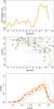 |
Fig. 1 Top: star formation rate history of the model. Middle: age-metallicity relation of the model, together with the stellar age and metallicities of the microlensing events of bulge stars from B13. Bottom: the metallicity distribution from the model (thin orange curve) and convolved with a Gaussian of 0.15 dex dispersion (thick orange curve) together with the generalized histograms of the observed MDF in Baade’s Window from Hill et al. (2011, thin dashed red curve) and shifted by −0.21 dex (thick dashed red curve), following the results of Rojas-Arriagada et al. (2014). |
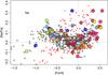 |
Fig. 2 Sodium abundance ratio as a function of [Fe/H] for stars in the disk (gray dots) from Bensby et al. (2014) and for stars in the bulge (larger symbols) from B13. The data from Johnson et al. (2014) are shown as red dots. |
The SFH, age-metallicity relation, and MDF distributions of Fig. 1 are used to generate the CMDs discussed in Sect. 3.
2.2. Galactic bulge SWEEPS field
Spatial segregation occurs in the bulge, with the most metal-poor (presumably older) populations dominating at larger distances from the Galactic plane, while in-plane fields are dominated by the most metal-rich (presumably the youngest) component (Ness et al. 2013). The field observed by CL08, Clarkson et al. (2011), and CA15 at l = 1.25° and b = −2.65° is 340 pc below the Galactic plane at the distance of the bulge (8 kpc). Hence, although the field is above the star formation layer, it may contain a significant number of stars that are a few Gyr old. However, young stars, if present, should be visible above the turn-off in the SWEEPS field, but no significant number have been detected (see CL08). Therefore, when we consider that the bulge may have a significant spread in age, we assume that stars are 3 Gyr old or older.
When we compare the data, a key ingredient is the metallicity distribution function. The MDF of the bulge is known to be a strong function of Galactic latitude (e.g., Ness et al. 2013), with the contribution of the metal-rich component decreasing at increasing latitude, but the spread in metallicity is wide throughout (Ness et al. 2013; Gonzalez et al. 2015).
According to Ness et al. (2013), the contribution of the metal-rich component (roughly [Fe/H] > 0.0 dex, their component A) is already as important as the medium metal-poor component (component B in Ness et al. 2013) at b = −5°. In Baade’s Window, the contribution of the metal-rich component is dominant (see, e.g., Gonzalez et al. 2015), with a strong peak at [Fe/H] ~ +0.25 dex, very similar to the model distribution of Fig. 1, and a spread from [Fe/H] = −1 to 0.7 dex. Metallicities measured from medium-resolution spectroscopy in the SWEEPS field for 93 stars show a similar spread from −1 to 0.8 dex, also compatible with other previous studies (Hill et al. 2011; B13; Ness et al. 2013; see Calamida et al. 2014 for more details). Our model MDF reproduces these main features fairly well: a wide spread in metallicity, and a prominent peak at super-solar metallicities, or [Fe/H] ~ +0.20 dex. Metallicities below −1.0 dex represent 5% of the total in the model MDF, while observed MDF often has a negligible amount of stars below this limit. To some part, this may be due to the small statistics of most surveys (a few hundred stars). Ness et al. (2013), whose study contained more objects by one order of magnitude than other surveys, showed the tail at [Fe/H] <−1.0 dex to be clearly visible, weighting about 1 ± 1% at b = −5° (Ness et al. 2013). In the following, we adopt the MDF of our model as a realistic representation of the MDF of the bulge in Baade’s Window or nearby SWEEPS fields, but also evaluate the photometric dispersion at the turn-off when discarding stars with [Fe/H] <−1.0 dex.
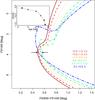 |
Fig. 3 Case (a): isochrones along the AMR of Fig. 1, also inset for ages 5, 7, 9, 10, and 13 Gyr. Corresponding metallicities and alpha abundances are indicated in the plot. The two arrows at the turn-off are separated by 0.07 mag. The age, metallicity, and [α/Fe] abundance are given for each isochrone. |
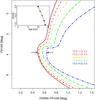 |
Fig. 4 Case (b): isochrones at 10, 11, 12, 13, and 13.5 Gyr and metallicities +0.3, 0.0, −0.5, −1.0, and −1.5 dex. The level of alpha elements is indicated in the plot. The two arrows at the turn-off are separated by 0.17 mag. The age, metallicity, and [α/Fe] abundance are plotted for each isochrone. |
In the CMD of CA15 (Fig. 4), the dispersion at the turn-off is 0.031 mag, and the spread, which we take as three standard deviations, is 0.093 mag (in the following, the term “dispersion” is used for standard deviation, while the “spread” is assumed as three times the dispersion and is taken as representative of the observed spread at the turn-off). The contribution of the photometric and data deduction technique to the spread is estimated to be 0.028 mag. Deducing this contribution of the observed dispersion, we obtain a dispersion of 0.0295 mag. This dispersion is due to age, metallicity, the contribution of binaries, differential extinction, and spread in distances of the stars. The intrinsic (due only to age and metallicity effects) dispersion at the turn-off is therefore extremely small and lower than 0.03 mag. We now seek to understand for which condition on age a synthetic CMD is compatible with such a narrow turn-off given the very wide distribution of metallicities observed in the bulge, and taking into account all the effects just mentioned through Monte Carlo simulations.
3. Color–magnitude diagram of the bulge
We have built CMDs considering three different cases. In case (a) the AMR is represented by our model. In case (b) the bulge is considered to be exclusively old (>10 Gyr), but a relation still links age to metallicity, while in case (c) we considered that stars are born in a burst and all have an age of 11 Gyr.
3.1. Isochrones
Figure 3 (case a) shows a set of isochrones in the (F814W, F606W−F814W) plane, covering the age range from 2 to 13.5 Gyr. Their metallicity is chosen according to the AMR of our model and is represented in the inset frame. The isochrones are calculated at the metallicity and alpha abundance content shown in each plot from the Yale library (Demarque et al. 2004). The conversion to the ACS-WFC F814W, F606W bands uses colors from the Dartmouth database (Dotter et al. 2008), which are based on Bedin et al. (2005). Although the age spanned by the isochrones is 11.5 Gyr (2 to 13.5 Gyr), the range in color in Fig. 3 at the turn-off of the old populations (F606W−F814W) is no more than ~0.08 mag between the isochrones at [Fe/H] = −1.5 (13.5 Gyr) and [Fe/H] = +0.35 dex (2 Gyr), which are the bluest and reddest turn-offs in Fig. 3, respectively. We note that because in case (a) the maximum metallicity considered is +0.35 dex, we also limited the spread in metallicity in case (b) and (c) to the same value. No metallicities higher than 0.35 dex were taken into account when we generated the CMDs below. Although it has no effect on case (a) because stars more metal-rich than +0.35 dex are also young, so they do not increase the spread at the turn-off (see the 2 Gyr isochrone in Fig. 3), this selection underestimates the intrinsic spread of case (b) and (c) by a few 0.01 mag at most, which strengthens the conclusions of this study.
Figure 4 (case b) shows an intermediate case where the bulge is represented by an AMR that extends from [Fe/H] = −1.5 dex at 13.5 to [Fe/H] = +0.5 dex at 10 Gyr. It is possible that while being old (>10 Gyr), the bulge would have such an AMR. In this case, the range in color is about twice the previous one, or about 0.17 mag.
Figure 5 (case c) shows a set of 11 Gyr isochrones with different metallicities (from −1.5 to +0.5). The plot illustrates that a coeval population, with a range of metallicities similar to what is observed for most of the bulge stars, has a wider turn-off (~0.2 mag) than the one presented in Fig. 3, as expected. These simple comparisons show that it is difficult to determine how the case for an old (either with an AMR or coeval) population can be compatible with observations, given that the observed photometric spread is smaller than 0.1 mag at the turn-off, while for case (b) and (c) it is larger than 0.17 mag.
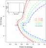 |
Fig. 5 Case (c): isochrones at age 11 Gyr and metallicities ranging from −1.5 to +0.5 dex. The two arrows at the turn-off are separated by 0.19 mag. The age, metallicity, and [α/Fe] abundance are plotted for each isochrone. |
Although a conclusion would be premature because several other effects have to be taken into account before comparing with the observed CMD (see following section), these results do suggest that given the broad range of metallicities found in the bulge, a uniformly old population (>10 Gyr) would produce a turn-off wider than observed in the studies of CL08, Clarkson et al. (2011), and CA15.
Figure 6 shows the set of isochrones of case (a) superposed on the CMD data of the SWEEPS field. Isochrones of age 13.5 and 2 Gyr are at the limit of the observed data points, but we do not expect many objects at these ages. Between 5 and 13 Gyr, the isochrones are well within the observed spread and illustrate that case (a) is perfectly possible.
Figure 7 shows different color plots from other isochrones (Dartmouth database, Dotter et al. 2008) to confirm the expected spread in color given the metallicity spread observed in the bulge using a set of different isochrones, but also to illustrate the expected intrinsic color range at the turn-off using different photometric bands from the HST-WFC3. The combination of F606W and F814W filters is best adapted to study this problem because this color maximizes the difference between the two extreme cases considered here (the case of a uniformly old population of age 11 Gyr and that of a spread of ~10 Gyr in age). Hence, although in absolute values the spread at the turn-off is wider in the F390W−F814W filters (1.29 mag compared to 0.21 mag in F606W−F814W for the no-AMR case), the spread is only twice as narrow in these filters for the AMR case (from 1.29 to 0.59 mag) but three times more narrow in F606W−F814W for the AMR case (from 0.21 to 0.074 mag). This means that the contrast between the cases with and without AMR is expected to be the highest in the F606W−F814W bands.
3.2. Simulated color–magnitude diagrams and comparison with the observations
We now illustrate this idea further by computing more realistic CMDs for the three cases presented in the previous section, taking the depth effect, the differential extinction, and binaries into account through Monte Carlo simulations. Starting from our model distributions, we simulate a set of (age, [Fe/H], [α/Fe]) parameters through Monte Carlo extraction from which we generate isochrones. A position along the isochrone is chosen according to the mass distribution generated from the IMF.
An extraction of ~10 000 stars was made for each case. The “intrinsic” dispersion (due to age and metallicity effects alone, no dispersion due to depth effects, binaries, or differential reddening) of each simulation is 0.026 (case a), 0.036 (b), and 0.044 mag (c). We note that these dispersions decrease to 0.023, 0.032, and 0.041 mag when only metallicities above −1.0 dex are selected, which shows that the tail at low metallicities has a limited effect. From these numbers, it is possible to see that the dispersion obtained for an isochrone population (case c) is hard to reconcile with the observations because it is already ~50% higher than the observed dispersion (~0.031 mag), given that none of the other sources of dispersion have been taken into account.
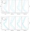 |
Fig. 7 Isochrones from Dartmouth at age 11 Gyr and metallicities ranging from −1.5 to +0.5 dex (top) and along the age-metallicity relation of Fig. 3 (bottom), in the theoretical CMD in different WFC3 colors. The horizontal short segment in each CMD is 0.2 mag long, to be compared with the width of the turn-off in each color band. The color separation at turn-off between the most metal-rich and metal-poor isochrones is 0.21 mag (top) and 0.074 mag (bottom) in the F606W−F814W, similarly to Figs. 5 and 3. The color separation at the turn-off is 0.333 and 0.124 mag in the F555W−F814W bands. Alpha abundances of the isochrones are the same as those used for the isochrones of Figs. 5 and 3. |
To obtain more realistic estimates, various contributions must be taken into account. The first is the depth effect: all stars are at different distances, and a variation of ±1 kpc at 8 kpc will translate into a difference in the distance modulus of about (+0.26, −0.29) mag. Following Valenti et al. (2013), a dispersion of 0.26 mag was added to take into account the spread in distance of stars in the bulge. The dispersion now rises to 0.035, 0.042, and 0.051 ± 0.001 mag, or a spread of 0.105, 0.126, and 0.153 mag.
Another potentially important effect that has to be taken into account comes from differential reddening. In CA15, this was taken into account by assuming a possible reddening variation of ±0.05 mag across the whole field, which we modeled by assuming a dispersion in reddening of 0.0166 mag. The resulting new dispersions are now 0.039 ± 0.0013, 0.045 ± 0.0009, and 0.054 ± 0.0012 mag, or a spread of 0.117, 0.135, and 0.162 mag for cases (a), (b), and (c) respectively (when metallicities are limited to [Fe/H] >−1.0 dex, the dispersions are 0.037 ± 0.0010, 0.043 ± 0.0011 and 0.051 ± 0.0012 mag).
The percentage of binaries and the distribution of their mass ratios is not known for the bulge. We simulated binaries by assuming a uniform distribution of mass ratios (Raghavan et al. 2010). Because the Yale stellar track library is limited to stellar masses higher than 0.4 M⊙, we derived unresolved binary parameters only when the companion has a mass higher than this limit. The mass at the turn-off is about 0.8 M⊙, which implies that companions with an absolute magnitude difference higher than about 4.5 mag are not modeled, corresponding to neglecting effects on combined magnitudes that are smaller than 0.015 mag, which is reasonable. According to CA15, the smallest fraction of binaries is about 30%, but it would easily reach 50% if it were similar to the disk (and if indeed the bulge is essentially made of disk stars). Assuming 30% of binaries, the dispersion increases to 0.051 ± 0.001 mag (case a), 0.056 ± 0.0019 (case b), and 0.064 ± 0.0015 mag (case c). These numbers rise to 0.056 ± 0.0014, 0.058 ± 0.0017 mag, and 0.065 ± 0.0014 for 50% binaries, and 0.056 ± 0.0013 mag (case a) 0.059 ± 0.0014 (case b), and 0.066 ± 0.0015 mag for 100% of binaries. The increase in dispersion is clearly not linear with the fraction of binaries, but varies most rapidly with low percentages, then flattens above 50%.
We conclude that even in case (a) the dispersion is higher than the one measured on the SWEEPS data, which means we have probably overestimated one or several of the sources of dispersion. Even so, it is difficult to imagine that the dispersion in cases (b) and (c) can be reconciled with a dispersion lower than 0.03 mag as the one observed, being already larger than this limit when only age and metallicity are taken into account. The freedom that we have to accommodate for a lower dispersion in case (a) is larger because, in addition to the possible overestimated differential reddening, distance uncertainty and effect of binaries, we neither tuned the AMR in any way nor the SFH, which both play a role in determining the dispersion at the turn-off.
In addition, we also note that the spread in color of the giant branch is also remarkably tight in Clarkson et al. (2011, their Fig. 1), being limited to at most 0.2 mag. This also agrees much better with case (a) than with case (c), where it can be seen that the spread is about 0.4 mag.
Hence, our study proves that the bulge must contain young disk stars in substantial amounts if we wish the spread of metallicities observed in several independent studies to be compatible with an apparently uniformly old bulge as observed from its CMD. If the bulge contains metal-rich stars, these have to be significantly younger than the subsolar metallicity population.
A final comment is worth making. We find that the CMD is not compatible with a unique (old) age given the spread in the metallicities, but this statement is true at all ages. In other words, the observed CMD is also a constraint on the dispersion of the age-metallicity relation in the inner disk and bulge and tells us that this relation must be relatively tight to accommodate the spread in color at the turn-off in the SWEEPS CMD. This is at variance with the age-metallicity relation observed at the solar vicinity, for example, but in accordance with the closed-box model we assumed for the inner disk and bulge. It tells us that the age-metallicity relation in the inner disk must be tighter, contrary to what is seen in the solar vicinity. Our interpretation is that because the solar vicinity is located in the transition region between the inner and outer disk, the metallicity gradient is very steep locally, bringing stars of significantly different metallicities at a given age in the local volume, while the evolution has been much more homogeneous in the inner disk.
4. Discussion
We have shown the following in this study:
-
(1)
A coeval stellar population with an age of11 Gyr and a metallicity distribution compatiblewith that of Baade’s Window implies a spread in the turn-off colorthat is significantly wider than the one observed in theSWEEPS field.
-
(2)
Even for a bulge with an age older than 10 Gyr and in which metallicity correlates with age, the turn-off region should be significantly broader than what is observed in the SWEEPS field.
-
(3)
A bulge population that is assumed to follow the same chemical characteristics (and in particular the same AMR) as those we used to model the inner disk (which is expected if the bulge is a bar formed from the disk) produces a CMD with a tight turn-off, hiding a spread in age of about 10 Gyr, between 3 and 13 Gyr.
These results imply that the currently known constraints from CL08 and Valenti et al. (2013) are not evidence that the bulge is exclusively old (>10 Gyr). On the contrary, they are evidence that the more metal-rich stars in the bulge must be significantly younger than the metal-poor ones, otherwise we would expect the turn-off of the bulge to be significantly broader than observed.
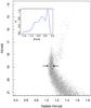 |
Fig. 8 Monte Carlo simulations of the CMD of Fig. 3 in the F814W/F606W−F814W bands, as described in the text. A dispersion of 0.26 mag has been applied on the magnitudes to take the spread in distance into account, 0.016 mag on colors to take the differential extinction into account, and 30% binaries. The two arrows in each plot correspond to a separation of 0.10 mag. The inset frame shows the corresponding metallicity distribution of the simulation. The percentage of objects younger than 9 Gyr in this plot is 34%. |
It is worth emphasizing here that we still view the bulge as predominantly old: in our model (see Haywood et al. 2016, and in prep.), about 50% of the stars must have ages greater than 9 Gyr. In the CMD of Fig. 8, the percentage of stars younger than 9 Gyr decreases to 34% because we considered that the SLEEPS field would have a negligeable amount of stars younger than 3 Gyr. Clearly, there is room for a younger population that makes up the bulk of the metal-rich peak. This population originates in the inner thin disk (see Di Matteo 2016, for a review), and its stars formed after the quenching episode (Haywood et al. 2016) that occurred at the end of thick-disk phase, and so they must be essentially younger than 8 Gyr.
Before discussing the evidence from the literature in favor of an exclusively old bulge, it is worth discussing the ages of the metal-rich dwarfs from B13 in light of our results and to determine in particular how far the ages of their metal-rich stars are still compatible, within the error bars, with being old (>10 Gyr), if we assume that they are all bulge stars. In their Fig. 4, of the 19 stars with [Fe/H] > 0.1 dex, 14 have ages compatible with being 5 Gyr old or younger within 1 sigma on Log Teff or log g, while only 5 are within one sigma of being 10 Gyr or older. All these 5 stars are also compatible with being younger than 10 Gyr (and for 3 of them, younger than 5 Gyr) within 1 or 2 sigmas. In contrast, 9 stars younger than 10 Gyr are irreconcilably hotter than the 10 Gyr isochrone, being sometimes off by more than 500 K (4 to 5σ on temperature). This is to emphasize the fact that while all metal-rich stars of B13 are reasonably (within 1 or 2 sigmas) compatible with being young (5 Gyr or younger), the reverse is not true, and no young star in B13 is compatible with being 10 Gyr old or older (within less than 4 to 5 sigmas on Log Teff), although this would be expected if the bulge were exclusively old. Finally, it is worth noting that Valle et al. (2015) redetermined the ages of the microlensed dwarfs in the sample of Bensby et al. (2013) using different methods and isochrones, and confirmed the fraction of young stars found by Bensby et al. (2013). We now review the arguments that have been invoked to support that the metal-rich population must be exclusively old.
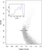 |
Fig. 9 Monte Carlo simulations of the CMD of Fig. 4 in the F814W/F606W−F814W bands, assuming the same conditions as in Fig. 8. The two arrows in each plot correspond to a separation of 0.15. The inset frame shows the corresponding metallicity distribution of the simulation. |
(1) Stellar population arguments
Until the 1990s, the Galactic bulge has been essentially associated to an old, collapsed component (e.g., Rich 1990; Matteucci & Brocato 1990), and it has been suggested that even its metal-rich stars might be older than the halo component (Renzini & Greggio 1990). Mainly two results have concurred to support the idea of a uniformly old bulge, even though the possibility of young super metal-rich stars has been recognized early (Wood & Bessell 1983). The first is the prediction by Matteucci & Brocato (1990) that alpha-enhanced abundances were to be expected even at high metallicities, and the first observations supported this prediction (McWilliam & Rich 1994). The second is the idea that the angular momentum distribution of the bulge is similar to the one of the halo – the thick disk having similar distribution to the thin disk – thereby linking the bulge to a primordial collapse of the Galaxy, see, for instance, Wyse & Gilmore (1992). While we discuss the chemical argument in more detail below, it is worth emphasizing that subsequent studies have not confirmed the substantially enhanced alpha abundances at solar metallicities and above.
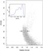 |
Fig. 10 Monte Carlo simulations of the CMD Fig. 5 in the F814W/F606W−F814W bands, assuming the same conditions as in Fig. 8. The two arrows in each plot correspond to a separation of 0.20 mag. The inset frame shows the corresponding metallicity distribution of the simulation. |
The discovery that the bulge is in fact a bar (Blitz & Spergel 1991) and the discovery that vertical instabilities create boxy and peanut-shaped morphologies (Combes & Sanders 1981) has prompted the idea that at least part of the bulge could be made of disk stars trapped in the bar, with the dual nature of the bulge already suggested at this time (Rich 1993). However, the measurement of alpha-enhanced abundances at high metallicities (McWilliam & Rich 1994; Lecureur et al. 2007) and the seemingly old CMD (CL08) suggested until recently that the bulge was a mixture of a classical and pseudo-bulge, prompting the presentation of more sophisticated chemical evolution models with a uniformly old bulge, even at high metallicities (Ballero et al. 2007; McWilliam et al. 2008).
It has been argued at the same time from kinematic arguments that if a classical bulge exists in the MW, it must either be small or nonexistent (Shen et al. 2010; Kunder et al. 2012; Di Matteo et al. 2014; Kunder et al. 2016 estimated its mass to be 1% of the total mass of the inner Galaxy). If the classical bulge is small, it implies that the bulge of the MW must be a pseudo-bulge, that is, a bulge formed from the disk through dynamical instabilities. The evidence that most of the bulge is a pseudo-bulge is now overwhelming. The last evidence came from the finding by McWilliam & Zoccali (2010) and Nataf et al. (2010) that the bulge is X-shaped. It has been shown in Di Matteo et al. (2014, 2015) how the disk inside the outer Linblad resonance radius can be mapped into the bar and how the stellar components detected by Ness et al. (2013) can be identified to belong to the thick and thin disks of the MW (Di Matteo 2016), while the peanut shape is seen to be most prominent in the metal-rich component (Ness et al. 2013), clearly indicating a disk origin.
This short summary shows that within little more than a decade, new data on the structural shape and kinematical characteristics have changed our view of the bulge from a collapsed, rapidly formed spheroidal component to a bar formed from dynamical instabilities in the disk. These arguments are not direct evidence that the metal-rich objects must be younger than ages expected for an old spheroid formed by mergers (as often advocated for a classical bulge), but they are evidence of a disk origin of these stars. Because there is no clue that metal-rich stars in the disk must be older than 10 Gyr, it is reasonable to expect that those seen in the bulge are also younger than this limit.
(2) Chemical argument
As mentioned previously, it has been argued that because the bulge is α-rich compared to the solar vicinity, it formed on a short timescale (e.g., Zoccali et al. 2006; Grieco et al. 2012). While it has been found in the first studies that metal-rich bulge stars seemed to be systematically more alpha-enhanced than local disk stars, the offset has only been decreasing in the past ten years. Most recently, studies made on the same types of stars (dwarfs) by the same group using the same method (B13 and Bensby et al. 2014) obtained results that are almost indistinguishable.
Johnson et al. (2012) argued that the low ratio of [La/Eu] indicates that the majority of the bulge formed rapidly (<1 Gyr). Figure 11 compares the [La/Eu] abundance ratio for two different bulge samples from Johnson et al. (2012) and Van der Swaelmen et al. (2016), together with three different samples of solar vicinity stars from Battistini & Bensby (2016), Mishenina et al. (2013), and Ishigaki et al. (2013). They agree well, and the two bulge samples show no evidence of having lower [La/Eu] than solar vicinity stars. We conclude that the available [La/Eu] abundance ratios do not provide evidence that the bulge formed faster than the inner disk. Other arguments are put in the balance for an old bulge by Nataf (2015), such as the presence of RR Lyrae and old globular clusters. However, they only confirm (if it was needed) that there are old populations in the bulge, but it does not imply that the bulge must be exclusively old.
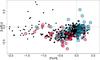 |
Fig. 11 [La/Eu] from Johnson et al. (2012) and Van der Swaelmen et al. (2016; pink and blue larger symbols, respectively) of bulge stars compared to data from Battistini & Bensby (2016; triangles), Mishenina et al. (2013; squares), and Ishigaki et al. (2013; diamonds) for solar vicinity stars. There is no evidence from this data that the bulge and the solar vicinity distributions are different. |
More generally, it is important to emphasize that there is no argument coming from chemical evolution modeling that would assert that the metal-rich population must be old. The original results from Matteucci & Brocato (1990) are based on endorsing a uniformly old age for the bulge (and particularly for metal-rich stars), which reflects the generally accepted idea of that time1. The most recent models of Galactic chemical evolution (GCE) are still trying to cope with representing the bulge as exclusively old, and the HST CMD of a seemingly old population has a heavy weight in this choice. Although they reproduce the observed chemical constraints reasonably well, we emphasize that (1) these models see the bulge as a component isolated from the disk, which is unrealistic given the present evidence of the bulge being mostly a pseudo-bulge; (2) modeling the bulge as an exclusively old and isolated system imposes a complexity and a number of ad hoc parameters that are not required by the data if the bulge is considered as a bar grown from the disk and having the age range of the disk. Grieco et al. (2012) modeled the metal-rich component with parameters different from those used for stars below [Fe/H] < 0.0 dex. The infall timescale, star formation efficiency, and IMF are assumed to be different from that of the stars at lower metallicities. Tsujimoto & Bekki (2012) formed the metal-rich component from gas at a metallicity [Fe/H] ~−0.3 dex, which, having to form stars on a short timescale, also implies a top-heavy IMF. GCE models are able to produce the metal-rich component as being exclusively old, but this comes with a price because forming stars enriched to [Fe/H] > +0.3 dex in a limited amount of time (within a few Gyr) is challenging. This is commonly done by endorsing a flatter IMF than the one used for the solar vicinity, for instance, a Salpeter IMF, or even flatter (Matteucci et al. 1999; Ballero et al. 2007; Tsujimoto & Bekki 2012; Grieco et al. 2012). In this context, it is worth mentioning that CA15 measured an IMF for the bulge population that is compatible with that of the disk and different from the Salpeter IMF. In addition, while it is sometimes recognized in these studies that the (metal-rich) bulge is a bar formed from disk material, these models still represent this component with specific and ad hoc parameters that differ from those adopted to reproduce the metal-poor component, but with little justification. For example, Grieco et al. (2012) formed metal-rich stars within less than 1 Gyr after the metal-poor population, but no argument justifies that the star formation efficiency is decreased by more than a factor of 10 (from 25 Gyr-1 to 2 Gyr-1) in such a short time or that the timescale for infall is increased by a factor of 30 (from 0.1 to 3 Gyr).
5. Conclusions
We conclude this study by saying that there is no evidence from the CMD in the SWEEPS field that would support that the bulge is exclusively old. The HST CMD has been claimed to provide the best evidence of an old bulge, but it is in fact evidence to the contrary: the tight turn-off of the CMD is possible only if it hides a correlation between age and metallicity, which means that metal-rich stars ([Fe/H] > 0) must be significantly younger than the metal-poor population ([Fe/H] < 0 dex). Haywood et al. (in prep.) will show that a model that represents the bulge with a thick and a thin disk reproduces observed chemical constraints well, without additional parameters except for those used to represent the thin and thick inner disks. Evidently, since we model the bulge with a thick+thin disk population, we release the constraint of ages greater than ~10 Gyr only. This facilitates the production of metal-rich stars, and in particular, there is no need to assume an IMF different from that of the disk. In our model, stars with [Fe/H] > 0 dex are all younger than 8 Gyr and are formed after the quenching episode (Haywood et al. 2016). Our results show that unless the MDF in the SWEEPS field is strongly different from that of the neighboring Baade Window, these younger stars are necessary to reproduce the CMD obtained from the HST.
This subject was then frequently discussed, see for example Frogel (1990): “whether or not the Galactic bulge contains a detectable population of stars with age much less than 10 Gyr is a subject of considerable debate”, to conclude that the bulge has no evidence for a population younger than 10 Gyr.
Acknowledgments
Based on observations made with the NASA/ESA Hubble Space Telescope, obtained by the Space Telescope Science Institute. STScI is operated by the Association of Universities for Research in Astronomy, Inc., under NASA contract NAS 5-26555. We are grateful to the referee for a detailed report and very helpful comments. A.C. acknowledges NASA, which supported her work through grants GO-9750 and GO-12586 from the Space Telescope Science Institute, which is operated by AURA, Inc., under NASA contract NAS 5-26555. The ANR (Agence Nationale de la Recherche) is acknowledged for its financial support through the MOD4Gaia project (ANR-15-CE31-0007).
References
- Ballero, S. K., Matteucci, F., Origlia, L., & Rich, R. M. 2007, A&A, 467, 123 [Google Scholar]
- Battistini, C., & Bensby, T. 2016, A&A, 586, A49 [NASA ADS] [CrossRef] [EDP Sciences] [Google Scholar]
- Bedin, L. R., Cassisi, S., Castelli, F., et al. 2005, MNRAS, 357, 1038 [NASA ADS] [CrossRef] [Google Scholar]
- Bensby, T., Adén, D., Meléndez, J., et al. 2011, A&A, 533, A134 [NASA ADS] [CrossRef] [EDP Sciences] [Google Scholar]
- Bensby, T., Yee, J. C., Feltzing, S., et al. 2013, A&A, 549, A147 [NASA ADS] [CrossRef] [EDP Sciences] [Google Scholar]
- Bensby, T., Feltzing, S., & Oey, M. S. 2014, A&A, 562, A71 [NASA ADS] [CrossRef] [EDP Sciences] [Google Scholar]
- Blitz, L., & Spergel, D. N. 1991, ApJ, 379, 631 [NASA ADS] [CrossRef] [Google Scholar]
- Calamida, A., Sahu, K. C., Anderson, J., et al. 2014, ApJ, 790, 164 [NASA ADS] [CrossRef] [Google Scholar]
- Calamida, A., Sahu, K. C., Casertano, S., et al. 2015, ApJ, 810, 8 [NASA ADS] [CrossRef] [Google Scholar]
- Clarkson, W., Sahu, K., Anderson, J., et al. 2008, ApJ, 684, 1110 [NASA ADS] [CrossRef] [Google Scholar]
- Clarkson, W. I., Sahu, K. C., Anderson, J., et al. 2011, ApJ, 735, 37 [NASA ADS] [CrossRef] [Google Scholar]
- Combes, F., & Sanders, R. H. 1981, A&A, 96, 164 [NASA ADS] [Google Scholar]
- Demarque, P., Woo, J.-H., Kim, Y.-C., & Yi, S. K. 2004, ApJS, 155, 667 [NASA ADS] [CrossRef] [Google Scholar]
- Di Matteo, P. 2016, PASA, 33, e027 [NASA ADS] [CrossRef] [Google Scholar]
- Di Matteo, P., Haywood, M., Gómez, A., et al. 2014, A&A, 567, A122 [NASA ADS] [CrossRef] [EDP Sciences] [Google Scholar]
- Di Matteo, P., Gómez, A., Haywood, M., et al. 2015, A&A, 577, A1 [NASA ADS] [CrossRef] [EDP Sciences] [Google Scholar]
- Dotter, A., Chaboyer, B., Jevremović, D., et al. 2008, ApJS, 178, 89 [NASA ADS] [CrossRef] [Google Scholar]
- Erwin, P., Saglia, R. P., Fabricius, M., et al. 2015, MNRAS, 446, 4039 [NASA ADS] [CrossRef] [Google Scholar]
- Fisher, D. B., & Drory, N. 2010, ApJ, 716, 942 [NASA ADS] [CrossRef] [Google Scholar]
- Fisher, D. B., & Drory, N. 2016, Galactic Bulges, 418, 41 [NASA ADS] [CrossRef] [Google Scholar]
- Frogel, J. A. 1990, European Southern Observatory Conference and Workshop Proceedings, 35, 177 [Google Scholar]
- Gonzalez, O. A., Zoccali, M., Vasquez, S., et al. 2015, A&A, 584, A46 [NASA ADS] [CrossRef] [EDP Sciences] [Google Scholar]
- Grieco, V., Matteucci, F., Pipino, A., & Cescutti, G. 2012, A&A, 548, A60 [NASA ADS] [CrossRef] [EDP Sciences] [Google Scholar]
- Haywood, M., Di Matteo, P., Lehnert, M. D., Katz, D., & Gómez, A. 2013, A&A, 560, A109 [NASA ADS] [CrossRef] [EDP Sciences] [Google Scholar]
- Haywood, M., Di Matteo, P., Snaith, O., & Lehnert, M. D. 2015, A&A, 579, A5 [NASA ADS] [CrossRef] [EDP Sciences] [Google Scholar]
- Haywood, M., Lehnert, M. D., Di Matteo, P., et al. 2016, A&A, 589, A66 [NASA ADS] [CrossRef] [EDP Sciences] [PubMed] [Google Scholar]
- Hill, V., Lecureur, A., Gómez, A., et al. 2011, A&A, 534, A80 [NASA ADS] [CrossRef] [EDP Sciences] [Google Scholar]
- Ishigaki, M. N., Aoki, W., & Chiba, M. 2013, ApJ, 771, 67 [NASA ADS] [CrossRef] [Google Scholar]
- Iwamoto, K., Brachwitz, F., Nomoto, K., et al. 1999, ApJS, 125, 439 [NASA ADS] [CrossRef] [MathSciNet] [Google Scholar]
- Johnson, C. I., Rich, R. M., Kobayashi, C., & Fulbright, J. P. 2012, ApJ, 749, 175 [NASA ADS] [CrossRef] [Google Scholar]
- Johnson, C. I., Rich, R. M., Kobayashi, C., Kunder, A., & Koch, A. 2014, AJ, 148, 67 [NASA ADS] [CrossRef] [Google Scholar]
- Karakas, A. I. 2010, MNRAS, 403, 1413 [NASA ADS] [CrossRef] [Google Scholar]
- Kormendy, J., & Kennicutt, R. C., Jr. 2004, ARA&A, 42, 603 [NASA ADS] [CrossRef] [Google Scholar]
- Kormendy, J., Drory, N., Bender, R., & Cornell, M. E. 2010, ApJ, 723, 54 [NASA ADS] [CrossRef] [Google Scholar]
- Kroupa, P. 2001, MNRAS, 322, 231 [NASA ADS] [CrossRef] [Google Scholar]
- Kunder, A., Koch, A., Rich, R. M., et al. 2012, AJ, 143, 57 [NASA ADS] [CrossRef] [Google Scholar]
- Kunder, A., Rich, R. M., Koch, A., et al. 2016, ApJ, 821, L25 [NASA ADS] [CrossRef] [Google Scholar]
- Lecureur, A., Hill, V., Zoccali, M., et al. 2007, A&A, 465, 799 [NASA ADS] [CrossRef] [EDP Sciences] [Google Scholar]
- Matteucci, F., & Brocato, E. 1990, ApJ, 365, 539 [NASA ADS] [CrossRef] [Google Scholar]
- Matteucci, F., Romano, D., & Molaro, P. 1999, A&A, 341, 458 [NASA ADS] [Google Scholar]
- McWilliam, A., & Rich, R. M. 1994, ApJS, 91, 749 [NASA ADS] [CrossRef] [Google Scholar]
- McWilliam, A., & Zoccali, M. 2010, ApJ, 724, 1491 [NASA ADS] [CrossRef] [Google Scholar]
- McWilliam, A., Matteucci, F., Ballero, S., et al. 2008, AJ, 136, 367 [NASA ADS] [CrossRef] [Google Scholar]
- Mishenina, T. V., Pignatari, M., Korotin, S. A., et al. 2013, A&A, 552, A128 [NASA ADS] [CrossRef] [EDP Sciences] [Google Scholar]
- Nataf, D. M. 2015, PASA, 33, e023 [Google Scholar]
- Nataf, D. M., Udalski, A., Gould, A., Fouqué, P., & Stanek, K. Z. 2010, ApJ, 721, L28 [NASA ADS] [CrossRef] [Google Scholar]
- Ness, M., Freeman, K., Athanassoula, E., et al. 2013, MNRAS, 430, 836 [NASA ADS] [CrossRef] [Google Scholar]
- Nomoto, K., Tominaga, N., Umeda, H., Kobayashi, C., & Maeda, K. 2006, Nucl. Phys. A, 777, 424 [NASA ADS] [CrossRef] [Google Scholar]
- Raghavan, D., McAlister, H. A., Henry, T. J., et al. 2010, ApJS, 190, 1 [NASA ADS] [CrossRef] [EDP Sciences] [Google Scholar]
- Raiteri, C. M., Villata, M., & Navarro, J. F. 1996, A&A, 315, 105 [NASA ADS] [Google Scholar]
- Renzini, A., & Greggio, L. 1990, European Southern Observatory Conference and Workshop Proceedings, 35, 47 [Google Scholar]
- Rich, R. M. 1990, ApJ, 362, 604 [NASA ADS] [CrossRef] [Google Scholar]
- Rich, R. M. 1993, Galaxy Evolution. The Milky Way Perspective, 49, 65 [NASA ADS] [Google Scholar]
- Rojas-Arriagada, A., Recio-Blanco, A., Hill, V., et al. 2014, A&A, 569, A103 [NASA ADS] [CrossRef] [EDP Sciences] [Google Scholar]
- Shen, J., Rich, R. M., Kormendy, J., et al. 2010, ApJ, 720, L72 [NASA ADS] [CrossRef] [Google Scholar]
- Snaith, O., Haywood, M., Di Matteo, P., et al. 2015, A&A, 578, A87 [NASA ADS] [CrossRef] [EDP Sciences] [Google Scholar]
- Tsujimoto, T., & Bekki, K. 2012, ApJ, 747, 125 [NASA ADS] [CrossRef] [Google Scholar]
- Valenti, E., Zoccali, M., Renzini, A., et al. 2013, A&A, 559, A98 [NASA ADS] [CrossRef] [EDP Sciences] [Google Scholar]
- Valle, G., Dell’Omodarme, M., Prada Moroni, P. G., & Degl’Innocenti, S. 2015, A&A, 577, A72 [NASA ADS] [CrossRef] [EDP Sciences] [Google Scholar]
- Van der Swaelmen, M., Barbuy, B., Hill, V., et al. 2016, A&A, 586, A1 [NASA ADS] [CrossRef] [EDP Sciences] [Google Scholar]
- van Loon, J. T., Gilmore, G. F., Omont, A., et al. 2003, MNRAS, 338, 857 [Google Scholar]
- Wood, P. R., & Bessell, M. S. 1983, ApJ, 265, 748 [NASA ADS] [CrossRef] [Google Scholar]
- Wyse, R. F. G., & Gilmore, G. 1992, AJ, 104, 144 [NASA ADS] [CrossRef] [Google Scholar]
- Zoccali, M., Lecureur, A., Barbuy, B., et al. 2006, A&A, 457, L1 [NASA ADS] [CrossRef] [EDP Sciences] [Google Scholar]
All Figures
|
Fig. 1 Top: star formation rate history of the model. Middle: age-metallicity relation of the model, together with the stellar age and metallicities of the microlensing events of bulge stars from B13. Bottom: the metallicity distribution from the model (thin orange curve) and convolved with a Gaussian of 0.15 dex dispersion (thick orange curve) together with the generalized histograms of the observed MDF in Baade’s Window from Hill et al. (2011, thin dashed red curve) and shifted by −0.21 dex (thick dashed red curve), following the results of Rojas-Arriagada et al. (2014). |
| In the text | |
|
Fig. 2 Sodium abundance ratio as a function of [Fe/H] for stars in the disk (gray dots) from Bensby et al. (2014) and for stars in the bulge (larger symbols) from B13. The data from Johnson et al. (2014) are shown as red dots. |
| In the text | |
|
Fig. 3 Case (a): isochrones along the AMR of Fig. 1, also inset for ages 5, 7, 9, 10, and 13 Gyr. Corresponding metallicities and alpha abundances are indicated in the plot. The two arrows at the turn-off are separated by 0.07 mag. The age, metallicity, and [α/Fe] abundance are given for each isochrone. |
| In the text | |
|
Fig. 4 Case (b): isochrones at 10, 11, 12, 13, and 13.5 Gyr and metallicities +0.3, 0.0, −0.5, −1.0, and −1.5 dex. The level of alpha elements is indicated in the plot. The two arrows at the turn-off are separated by 0.17 mag. The age, metallicity, and [α/Fe] abundance are plotted for each isochrone. |
| In the text | |
|
Fig. 5 Case (c): isochrones at age 11 Gyr and metallicities ranging from −1.5 to +0.5 dex. The two arrows at the turn-off are separated by 0.19 mag. The age, metallicity, and [α/Fe] abundance are plotted for each isochrone. |
| In the text | |
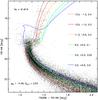 |
Fig. 6 CMD in the SWEEPS field together with the isochrones of Fig. 3. |
| In the text | |
|
Fig. 7 Isochrones from Dartmouth at age 11 Gyr and metallicities ranging from −1.5 to +0.5 dex (top) and along the age-metallicity relation of Fig. 3 (bottom), in the theoretical CMD in different WFC3 colors. The horizontal short segment in each CMD is 0.2 mag long, to be compared with the width of the turn-off in each color band. The color separation at turn-off between the most metal-rich and metal-poor isochrones is 0.21 mag (top) and 0.074 mag (bottom) in the F606W−F814W, similarly to Figs. 5 and 3. The color separation at the turn-off is 0.333 and 0.124 mag in the F555W−F814W bands. Alpha abundances of the isochrones are the same as those used for the isochrones of Figs. 5 and 3. |
| In the text | |
|
Fig. 8 Monte Carlo simulations of the CMD of Fig. 3 in the F814W/F606W−F814W bands, as described in the text. A dispersion of 0.26 mag has been applied on the magnitudes to take the spread in distance into account, 0.016 mag on colors to take the differential extinction into account, and 30% binaries. The two arrows in each plot correspond to a separation of 0.10 mag. The inset frame shows the corresponding metallicity distribution of the simulation. The percentage of objects younger than 9 Gyr in this plot is 34%. |
| In the text | |
|
Fig. 9 Monte Carlo simulations of the CMD of Fig. 4 in the F814W/F606W−F814W bands, assuming the same conditions as in Fig. 8. The two arrows in each plot correspond to a separation of 0.15. The inset frame shows the corresponding metallicity distribution of the simulation. |
| In the text | |
|
Fig. 10 Monte Carlo simulations of the CMD Fig. 5 in the F814W/F606W−F814W bands, assuming the same conditions as in Fig. 8. The two arrows in each plot correspond to a separation of 0.20 mag. The inset frame shows the corresponding metallicity distribution of the simulation. |
| In the text | |
|
Fig. 11 [La/Eu] from Johnson et al. (2012) and Van der Swaelmen et al. (2016; pink and blue larger symbols, respectively) of bulge stars compared to data from Battistini & Bensby (2016; triangles), Mishenina et al. (2013; squares), and Ishigaki et al. (2013; diamonds) for solar vicinity stars. There is no evidence from this data that the bulge and the solar vicinity distributions are different. |
| In the text | |
Current usage metrics show cumulative count of Article Views (full-text article views including HTML views, PDF and ePub downloads, according to the available data) and Abstracts Views on Vision4Press platform.
Data correspond to usage on the plateform after 2015. The current usage metrics is available 48-96 hours after online publication and is updated daily on week days.
Initial download of the metrics may take a while.