| Issue |
A&A
Volume 592, August 2016
|
|
|---|---|---|
| Article Number | A144 | |
| Number of page(s) | 12 | |
| Section | Stellar structure and evolution | |
| DOI | https://doi.org/10.1051/0004-6361/201628855 | |
| Published online | 17 August 2016 | |
The SERMON project: 48 new field Blazhko stars and an investigation of modulation-period distribution
1 Konkoly
Observatory, MTA Research Centre for
Astronomy and Earth Sciences, Konkoly Thege Miklós út 15−17, 1121 Budapest, Hungary
e-mail: This email address is being protected from spambots. You need JavaScript enabled to view it.
2 Department of Theoretical Physics and
Astrophysics, Masaryk University, Kotlářská 2, 611
37
Brno, Czech
Republic
3 Variable Star and Exoplanet Section
of the Czech Astronomical Society, Valašské Meziříčí, Vsetínská 78,
757 01
Valašské Meziříčí, Czech
Republic
Received:
4
May
2016
Accepted:
13
June
2016
Abstract
Aims. We investigated 1234 fundamental mode RR Lyrae stars observed by the All Sky Automated Survey (ASAS) to identify the Blazhko (BL) effect. A sample of 1547 BL stars from the literature was collected to compare the modulation-period distribution with stars newly identified in our sample.
Methods. A classical frequency spectra analysis was performed using Period04 software. Data points from each star from the ASAS database were analysed individually to avoid confusion with artificial peaks and aliases. Statistical methods were used in the investigation of the modulation-period distribution.
Results. Altogether we identified 87 BL stars (48 new detections), 7 candidate stars, and 22 stars showing long-term period variations. The distribution of modulation periods of newly identified BL stars corresponds well to the distribution of modulation periods of stars located in the Galactic field, Galactic bulge, Large Magellanic Cloud, and globular cluster M5 collected from the literature. As a very important by-product of this comparison, we found that pulsation periods of BL stars follow Gaussian distribution with the mean period of 0.54 ± 0.07 d, while the modulation periods show log-normal distribution with centre at log (Pm [d]) = 1.78 ± 0.30 dex. This means that 99.7% of all known modulated stars have BL periods between 7.6 and 478 days. We discuss the identification of long modulation periods and show, that a significant percentage of stars showing long-term period variations could be classified as BL stars.
Key words: stars: variables: RR Lyrae / stars: horizontal-branch / methods: statistical
© ESO 2016
1. Introduction
Together with ultra-precise space measurements from the Kepler and CoRoT telescopes, the large-scale surveys play crucial role in investigation of long-term amplitude and frequency (phase) modulation in RR Lyrae stars known as the Blazhko (BL) effect (Blažko 1907). Accurate space data helped uncover various dynamical processes present only in modulated stars (for example, period doubling (Szabó et al. 2010; Kolláth et al. 2011) and additional radial and non-radial modes Benkő et al. 2014; Szabó et al. 2014). Data from the ground-based surveys, on the other hand, are very useful for studying large samples statistically and investigating general and common characteristics of modulated stars (e.g. Alcock et al. 2003; Soszyński et al. 2011).
Both approaches are important in their own way because the nature of the BL effect has not been fully explained yet. The true percentage of modulated stars is still unknown (see e.g. Jurcsik et al. 2009; Kovács 2016). Even more interestingly, it is not clear why some stars show modulation and some with very similar physical properties do not (e.g. Skarka 2014b). Knowledge about characteristics of the BL effect is still insufficient to give a reliable answer to the question of if and how the pulsation period is connected with the length and amplitude of the modulation. Jurcsik et al. (2005a) showed that the modulation amplitude of short-pulsation-period RR Lyrae stars can be higher than for long-period stars. Benkő et al. (2014) and Benkő & Szabó (2015) suggest a monotonic dependence between the strength of amplitude modulation and the period of the BL cycle (the longer the cycle, the larger the amplitude). While the upper limit of the modulation length is still unclear, the bottom limit is probably defined by the upper limit of the rotational velocity of a star. RR Lyrae stars with short pulsation periods can have short modulation periods, while long-pulsation-period stars can only have a BL cycle that is longer than about 20 d (Jurcsik et al. 2005b).
Several studies report on the mode switching and (or) disappearing (reappearing) of the BL effect, suggesting that the phenomenon could be of temporal nature (see e.g. Szeidl 1976; Sódor et al. 2007; Goranskij et al. 2010; Jurcsik et al. 2012; Plachy et al. 2014). Many stars also show variations of their modulation cycles (see e.g. Guggenberger et al. 2012; Benkő et al. 2014; Szabó et al. 2014). In some BL stars, for example in RR Lyrae itself, the modulation reappears cyclically during an additional four-year cycle (Detre & Szeidl 1973; Le Borgne et al. 2014; Poretti et al. 2016). There are many more interesting features of the BL effect. Extensive reviews of the BL effect are provided in recent overviews by Szabó (2014), Kovács (2016), and Smolec (2016).
In his study based on the brightest RRab stars observed by the All Sky Automated Survey (ASAS; e.g. Pojmański 1997, 2001) and the Super Wide Angle Search for Planets (SuperWASP; Pollacco et al. 2006), Skarka (2014a) revealed the shortcomings of current automated procedures dedicated for the search for the BL effect and the need for permanent supervision of all steps when analysing noisy ground-based data dominated by various aliases. His study also showed that there are many undiscovered modulated stars even in previously studied data sets. Because frequency analysis and searching for the manifestations of the BL effect in many targets individually is a very time-consuming task, we establish a new group involving professionals, students, and amateur astronomers that aim to analyse data from various surveys. The project was called SERMON which is the abbreviation of SEarch for Rr lyraes with MOdulatioN.
In this paper we focus on RRab stars observed by ASAS that are brighter than 13.5 mag in maximum light to investigate their frequency spectra trying to reveal the BL effect. Because the ASAS data have special characteristics and need special handling, we describe these data in detail in Sect. 2. We also describe the sample selection in this section. Analysis, criteria for the detection of the BL effect and discussion about the sample stars are described in Sect. 3. In Sect. 4 we investigate the distribution of modulation periods. The results are discussed in Sect. 5, the content of the paper is summarized in Sect. 6.
2. The ASAS data
The ASAS-3 survey is performed by small-aperture telescopes that are primarily dedicated to search for new variables among stars with declination below + 28° (technical details can be found in Pojmański 2001). The telescopes regularly scan the sky, and typically observe a particular object once per a few days with a three-minute exposure in V filter.
The publicly available data typically contain several hundreds of data points, which are marked with flags from A (the best quality) to D (the worst quality). The photometry often consists of several blocks in the data files because each star is usually observed in a few different fields. Magnitudes with errors are provided in five apertures with diameter between 2 and 6 pixels. The time span of the data is about 3300 days in most cases.
The philosophy of the survey has a deep impact on data characteristics. Low sampling rate causes the frequency spectra to be strongly dominated by daily aliases (Fig. 1). Because the angular resolution of the ASAS instruments is very low (about 15 arcsec/pixel), even with the smallest aperture the light of the target star could be influenced by neighbouring star(s), which is (are) closer than 30 arcsec. This fact could seriously bias the data. We discuss this problem in detail in Appendix A. An extensive overview of the ASAS data characteristics can be found in Pigulski (2014).
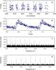 |
Fig. 1 Typical ASAS data demonstrated on V1124 Her. Panels a) and b) show the data distribution and data phased with the basic pulsation period. Panel c) shows corresponding frequency spectrum; panel d) shows the spectral window. |
2.1. The sample selection and data cleaning
This paper represents the extension of the study by Skarka (2014a) with fainter stars and stars with more scattered data. To some extend it complements the analysis by Szczygieł & Fabrycky (2007) who performed an automatic search on the full sample of all types of RR Lyrae stars in the ASAS Catalogue of Variable Stars (ACVS).
Stars identified as modulated for the first time.
The selection process started with the International Variable Star indeX catalogue (VSX; Watson et al. 2006, version from 27th October, 2014), in which 1760 stars of RRab type with maximum light brighter than 13.5 mag and declination below +28° were listed. The declination limit is given by the observational constraints of the ASAS survey. The magnitude limit was chosen according to several tests as the most limiting for reliable analysis because the scatter steeply increases with decreasing brightness. The corresponding photometric error of a data point at 13.5 mag is about 0.15 mag (Pojmański 2002).
Stars analysed by Skarka (2014a) were ignored. Then we checked for the availability of the data via the online VSX tools. This resulted in 1435 stars that were observed by ASAS. After downloading the data, we obtained a basic idea about the quality of the data, checked for possible blends in the area with diameter of 30 arcsec, and made a note (col. Blend in Tables 1, B.4, B.5, and col. Rem in Table 2). We used only data with flags A and B in aperture with the smallest average photometry error. Possible shifts in the mean magnitude between blocks were ignored because of the poor data sampling and problems with blends. All points that differed more than 1.5 mag from the median value were automatically removed. No other automatic procedure was applied for improving the data to avoid possible misinterpretation because, for example, scatter caused by modulation could be very easily confused with observational scatter.
In the next step, all stars with less than 150 points were discarded. Then we performed a visual inspection of all light curves again, and searched for the basic pulsation period in stars where the value given in VSX was not reliable. In stars where suitable period was found (or was available in VSX) obvious outliers were manually deleted. Stars with extremely scattered data were removed from the sample. This kind of pre-analysis gave us an idea about some peculiarities in the objects and allowed us to identify duplicates (Sect. 3.4) and stars of different variable types (Sect. 3.5). Together with these peculiar objects the sample for further analysis contained 1234 stars.
3. Analysis and identification of the BL stars
A mathematical description of simultaneous amplitude and phase (frequency) modulation suggests the rise of an additional peak with modulation frequency (fm) and equidistant peaks near the basic pulsation frequency components (kf0 ± fm; for details see Benkő et al. 2011; Szeidl et al. 2012). This equidistant spacing is equivalent to fm. Because the presence of the side peaks in the frequency spectra is the most distinct and convincing evidence of the BL effect, which is also detectable in scattered data, we searched for this feature using Period04 software (Lenz & Breger 2005). Owing to the characteristics of the data, it was necessary to pay special attention to properly identify correct peaks and avoid possible confusion with aliases.
It is likely that variable contamination with parasite light from nearby stars entering the aperture could resemble the amplitude modulation in some of the sample stars. In such cases, the mean magnitude and total amplitude of the light variations varies in time and produces conspicuous peak in the low-frequency range of the frequency spectrum. A visual check of the data itself would not help much because of large scatter and poor sampling, and statistics fails too for the same reasons. Therefore, the only way to reveal this issue is to identify the false modulation peak. No such peak was observed in any of the sample stars, however, we cannot exclude that some of the stars could be influenced by this problem. This is one of the reasons why we give the information about blends in the tables.
A star was marked as a BL star when a peak with S/N> 3.5 in the interval of f0 ± 0.2 c/d was identified. It was found by Nagy & Kovács (2006) that in stars with frequency separation of less than 1.5/TS (periods longer than 2/3TS), where TS is the time span of the data, it is impossible to distinguish unambiguously between BL modulation and long-term continuous period change (instability) of the main pulsation period (i.e. period-change stars, PC class, as described in the next paragraph). Therefore, only peaks with separation larger than 1.5/TS were considered a consequence of the BL effect. An example of the frequency spectrum for a BL star is shown in the left-hand panel of Fig. 2, where an equidistant triplet is seen.
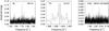 |
Fig. 2 Typical frequency spectra after prewhitening with the basic pulsation components for BL stars, PC, and candidate stars (from left to the right). The position of the basic pulsation frequency is shown with the red dashed line. |
The second category that we adopted is a PC group. Stars assigned to this group are usually those showing either unresolved peaks (peaks with frequency distance lower than 1/TS), or it is impossible to prewhiten the peaks in a few consecutive steps (Alcock et al. 2000; Nagy & Kovács 2006). Following our period limit for BL stars, each star with frequency separation lower than 1.5/TS was assigned to PC class as well. However, it is sometimes difficult to properly decide about BL/PC category, thus, we adopted these conservative criteria to make sure that PC stars do not contaminate significantly our BL sample (see also the discussion in Sect. 5). A typical frequency spectrum of a PC star is shown in the middle panel of Fig. 2.
Finally, we use candidate category for stars that would belong to the BL group, but the peaks have amplitudes under the detection limit or very close to integer daily frequencies (1 c/d, 2 c/d etc., the right-hand panel of Fig. 2).
3.1. Stars with the BL effect
An online version of the BlaSGalF database1 containing Galactic field RR Lyrae stars with the BL effect reported in literature contains 58 stars from our sample (version from 29th February, 2016, Skarka 2013). We detected the side peak in only 39 of these stars (see Table B.4). One of these 58 stars belongs to our candidate category, one was found to be of different variability type, and one star is a PC star. In remaining 16 stars we did not detect any peak possibly related to modulation (see Table B.1).
Although we cannot be sure in 100 percent of the stars, we assume, that the nondetection of the BL effect is a consequence of the data characteristics rather then the result of absence of the BL effect. We found two reasons for that. First, the noise level of the residuals after removing significant frequencies is typically between 0.01 and 0.02 mag, which means that sometimes side peaks with amplitude below ~0.07 mag do not fulfil S/N> 3.5. Second, some of the stars surely showed large-amplitude BL effect at the times when ASAS gathered the data. For example, Jurcsik et al. (2009) easily detected the modulation in the frequency spectra of AQ Lyr and UZ Vir using high-quality photometric observations gathered with a 60-cm telescope between 2004 and 2009. They also did not detect any clear sign of modulation in ASAS and NSVS data that is confirmed by our analysis. In any case, the nondetection of the BL effect in ASAS data should not be considered as a proof of the absence of the modulation.
In 48 stars the BL effect was detected for the first time (see Table 1). In addition to the information about pulsation and modulation periods resulting from our analysis (Cols. 2 and 3) and corresponding errors in the last digits in parentheses, we give information about nearby stars closer than 30 arcsec (18 objects with “+” in col. 5 named Blend), and about the number of data points and the time span of the data (Cols. 6 N and 7 TS). Four stars denoted with “+” in the last column Rem, in which we detected additional, either unresolved, or unique peaks close to kf0, are suspected of multiple modulation (category νM from Alcock et al. 2003 and MC from Nagy & Kovács 2006), or additional long-period variation. Instead of amplitudes of the side peaks, which could be influenced by nearby stars, we give S/N in the fourth column. Errors of periods (in all tables) are 2σ formal uncertainties from the least-squares fitting method.
Stars showing close, unresolved peaks near f0 that were marked as PC.
All data of newly identified modulated stars phased with the modulation periods from Table 1 are shown in Fig. 3. In most of the stars the modulation envelope is well apparent. This figure also shows a variety of envelope shapes and modulation amplitudes. Some of the stars, for example ASAS J181510-3545.7 and V0420 Vel, have very small total amplitudes compared to the other stars, which is most likely a result of blends with nearby stars.
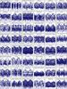 |
Fig. 3 BL stars phased with modulation periods from Table 1. As the zero epoch we simply took HJD of the brightest data point. Ticks at the ordinate show interval of 0.2 mag, at abscissa the interval is 0.5 in BL phase. |
3.2. Stars with unresolved peaks
Our 22 PC stars are listed in Table 2. The modulation periods suggested by the frequency spacing range from 1900 d in BK Eri to 4000 d in SV Eri. The latter is a star with the most rapid period change known among RR Lyrae stars so far (Poretti et al. 2016). When the data are phased with the suggested modulation periods, DI Aps, QZ Cen, V0584 Cen, NSVS 14009, V0898 Mon, and V0687 Pup show apparent amplitude changes. It may be possible that in a data set with long enough time span, these stars will turn out to be classical BL stars with very long modulation periods (see also Sect. 5 and Fig. 7.)
Short pulsation periods of ASASJ 054843-1627.0, J160612-4319.2 and their low amplitude and phase Fourier coefficients (transformed to I-band filter) suggest that they are of RRc type when compared to characteristics of Galactic bulge RR Lyrae parameters provided by Soszyński et al. (2011).
3.3. Candidates for BL stars
In seven stars we noticed peaks within f0 ± 0.2 c/d, but we mark them as candidates from the reasons discussed previously. In YZ Aps, NSVS 15218045 (see Fig. 2), ASAS J054238-2557.3, and V1211 Sgr, the suspicious peaks were very close to integer multiples of 1 c/d, which is always problematic. In ASAS J081549-0732.9 and ASAS J194745-4539.7 only peaks with S/N< 3.5 were detected.
3.4. Duplicates
During our analysis we identified three stars as duplicates because a star with a different ID is located almost at the same coordinates and it has similar pulsation (variability) properties. Actually, this was a trigger to perform a detail analysis of this problem regarding the total VSX catalogue (Liška et al. 2015). Our duplicates are given in Table B.3.
3.5. Stars with different variable type
In 24 stars (Table B.2 in Appendix B) we detected no signs of variability, 19 other stars are probably not RRab stars, but we suspect that they are of different variability type (Table B.5, Fig. B.1). We give suggested variability types that were estimated on the basis of period, light-curve shape, and B − V (Table B.5, Fig. B.1).
3.6. Characteristics of sample BL stars
The percentage of all BL stars in our sample (both known + new detections) is very low, at slightly less than 7%. The reason is a large scatter that could hider the modulation, rather than a real lack of modulated stars among faint stars. Therefore, this number has nothing to do with the real amount of modulated stars, but only gives information about the detectability of modulation in the data set. Our assumption is reinforced by the look of the magnitude distribution of the sample stars shown in Fig. 4 (see the percentages above bins). The highest number of BL stars was detected between 12.5 and 13.0 mag 2 and decreases steeply in the most populated area with faint stars with scattered data.
In the majority of the new BL stars the modulation is very apparent causing large amplitude changes (e.g. BW CMa, V0484 Ser), while in some of the stars the modulation in amplitude is barely seen (e.g. NSV 14546, SS Pic, see Fig. 3). Even in scattered ASAS data, a wide palette of the shapes of modulation envelopes is apparent. In this sense, one of the most interesting examples is UW Hor, which seems to show non-sinusoidal amplitude modulation. On the other hand, BN Oct and ASAS J162246-6723.5 show nearly sinusoidal variations in amplitude. The BL peak fm itself was detected only in BL Col, a known BL star. In four new BL stars and three PC stars we detected additional peaks, which could be interpreted as additional modulation, or signs of additional period change. Unfortunately, the low quality of the data does not allow us to investigate these peculiarities in detail.
4. Modulation-period distribution
To get an idea about the new BL stars, we collected a sample of 1547 fundamental mode stars with estimated modulation period from the literature. This sample contains RRab stars from the Galactic field (246 stars from the BlaSGalF database; Skarka 2013), the LMC (731 stars; Alcock et al. 2003), the Galactic bulge (19+526 stars; Moskalik & Poretti 2003; Collinge et al. 2006), and globular cluster M5 (25 stars; Jurcsik et al. 2011). We considered all periods in stars with multiple modulation. For example, from RS Boo we have three values on our list. Together with our new detections (48), it amounts 1628 entries, which is, to our knowledge, the most extended sample of modulation periods investigated so far.
The modulation periods of newly identified BL stars (black circles in the top panel of Fig. 5) match the distribution very well, and no sample star has extreme modulation period3. Two of our stars with the shortest modulation period, ASAS J175143+1708.4 and ASAS J112830-2429.7, however, seem to significantly differ from the general trend. The BL effect in these two stars should be proved independently. Light curve shape, pulsation period of only about 0.35 d, and its Fourier parameters suggest that NSV 14546 could be an RRc-type rather than RRab-type star.
To test the similarity of our sample with the sample of stars from literature, we performed the two-sample Kolmogorov-Smirnov test. The result is, that the agreement between the two populations cannot be ruled out with probability of 7%. Thus we can conclude that our sample stars have a similar distribution of modulation periods as BL stars from literature (see the cumulative-distribution functions in the right-hand panel of Fig. 6).
However, the modulation-period distribution in Fig. 5 itself is far more interesting than the distribution of new BL stars4. While pulsation periods show a distribution close to the normal Gaussian distribution (the bottom part of the top panel in Fig. 5), modulation periods follow the log-normal distribution. In other words, they show normal distribution when the BL periods are plotted in logarithmic scale, which is nicely seen from the bottom panel of Fig. 5 and histograms in the left-hand panel of Fig. 6. The mean pulsation period of BL stars is 0.54 ± 0.07 d, and the mean modulation period based on the log-normal distribution is 1.78 ± 0.30 dex. This means that 99.7% (3σ interval) of all BL stars have modulation periods between 7.6 and 478 days.
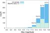 |
Fig. 4 Magnitude distribution of all sample stars (blue) and BL stars (green grid). The distribution of modulated stars was enlarged five times for better visibility. |
5. Discussion
The log-normal distribution commonly appears in measured quantities that cannot be negative. Many of natural, social, and technical systems and quantities show such distribution, for example the length of a latent infection (from infection to burst of the disease), species abundance, age of marriage, and probability of failure of mechanical devices (nice examples across the disciplines can be found in Limpert et al. 2001). The question is why the pulsation periods have Gaussian distribution, while modulation periods show log-normal distribution. Why do the majority of BL stars have modulation periods between 30 and 120 days (1σ interval)? At the present time, it is impossible to answer this question because no correlation between any of the physical characteristics and the length of the modulation period has been found.
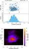 |
Fig. 5 BL period as a function of the pulsation period for known and new modulated stars (top), and corresponding density plot (bottom). The bottom part of the top panel shows the distribution of pulsation periods. |
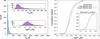 |
Fig. 6 Distribution of modulation periods (left-hand panel) and cumulative distribution functions (right-hand panel). It is apparent that the overall distribution follows the log-normal distribution. The agreement with the normal distribution for stars with modulation periods between 0 and 400 days shown in the insert in the right-hand panel is very good. |
The selection effects only have minor impact on the distribution, if any. The majority of used BL stars come from the data sets with time span that is several years long, where the modulation periods of several hundreds of days should be safely detectable. Yearly aliases cause problems with identification only in a very small part of the distribution (see the gap around 350 d in the top insert in the left-hand panel of Fig. 6). Thus we are convinced that the log-normal distribution is real. The very good agreement between the cumulative-distribution function for the periods in this interval and the normal distribution with the same parameters also confirms our assumption (the insert in the right-hand panel of Fig. 6).
It seems that the log-normal distribution only represents the short-period part of the modulation period distribution well (0−400 d), which has a long tail towards longer modulation periods. However, the distribution of the longest BL periods, which is probably much more numerous than our collection shows, is somewhat uncertain from several reasons. First, the entire sample is sharply cut at BL periods of about log Pm ~ 3.5 (~3300 d). This limit is given by the extension of the longest data used for modulation period estimation (the ASAS-3 data with maximum time span of about 3300 days). Data from MACHO survey has time span of about 7.5 yrs. It can be naturally expected that the distribution continues to even longer modulation periods because we do not know the upper limit. What is probably the longest BL effect with period longer than 25 yrs is reported by Jurcsik & Smitola (2016) in V144 in globular cluster M3.
Recent observational investigations (e.g. Benkő et al. 2014) showed that the BL stars always show both amplitude and phase variations. The BL stars could then be identified through the variations in amplitude even when the modulation period is comparable with TS, or longer. For example, V0898 Mon and V0687 Pup from our sample (top panels of Fig. 7) show significant amplitude changes with suggested periods that are a bit longer than 2/3TS. Although the modulation periods are only very roughly estimated in these stars, the BL-phased light curves suggest, that they could safely be considered BL stars.
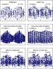 |
Fig. 7 Stars originally classified as pure PC. There are stars from our sample in the top panels. The middle panels show OGLE-III data demonstrating that in long-enough data sets (original classification comes from OGLE-II data with three-times shorter time span) the stars could be classified as BL stars, not pure PC stars. The bottom panels show two stars that clearly show amplitude modulation with periods shorter than 2/3TS suggesting classification as BL+PC, not pure PC. The scales of the axes are the same as in Fig. 3. |
Another uncertainty relies in the problems with the BL/PC classification. Although secular period changes and nonstationarity in pulsation period are quite common among RR Lyrae stars (see e.g. Le Borgne et al. 2007), we can expect a significant number of PC stars to be classified as BL stars in long-enough data sets. This is, for example, the case of OGLE-BLG-RRLYR-07697 and OGLE-BLG-RRLYR-06232. These two stars were classified as pure PC stars by Collinge et al. (2006) on the basis of the four-year-long OGLE-II data. In OGLE-III data (Soszyński et al. 2011), with a time span of about 12 yrs, these two stars appeared to be clear BL stars showing significant amplitude modulation with periods of 1300 and 2200 d (the middle panels of Fig. 7). In OGLE-BLG-RRLYR-07697 the side peaks were easily prewhitenable5. In OGLE-BLG-RRLYR-06232 we detected additional, unresolved structures very close to f0, which cannot be fully eliminated, thus, suggesting some additional period variations. According to the criteria adopted in Sect. 3, this star should be classified as both BL and PC star.
Further, we also suppose that stars showing dense patterns close to f0, which cannot be prewhitened in a few steps, do not necessarily exclude the possibility of being BL stars. In the bottom panel of Fig. 7 we see two stars identified as pure PC stars on the basis of MACHO data (Alcock et al. 2003). Both of these stars clearly show large amplitude modulation with periods shorter than 2/3TS. Thus, there is no reason why we do not assign them to the BL class with a possible additional PC component. It would be advisable to strictly distinguish between unresolved peaks close to f0, which could mean instability of the main pulsation period, and other unresolved peaks near the side peaks, which in turn could mean the nonstationarity of the modulation itself, additional modulation, or some artificially generated periodicity in the data. In such cases the star should be classified as BL star with additional PC, rather then pure PC.
As many previous investigations show (LaCluyzé et al. 2004; Sódor et al. 2007; Detre & Szeidl 1973; Szeidl 1976; Le Borgne et al. 2014; Guggenberger et al. 2012), the BL modulation itself can change on year-long time scale. Although the ASAS and MACHO data sets span rather long time bases, they typically do not contain sufficient number of data points to investigate such details. Therefore, many stars with changing BL modulation might remain undetected or classified as PC stars. These very few examples show that the distribution of modulation periods that are longer than ~1000 d is certainly more populated than we see in Fig. 6.
6. Summary and conclusions
We performed an in-depth study of frequency spectra of 1234 fundamental RR Lyrae stars observed by the ASAS survey, placing emphasis on proper identification of possible modulation. Therefore, we investigated each target individually within a new project SERMON employing professionals, amateurs, and students. We omitted stars with a low number of points (<150) and scattered light curves with insufficient quality for period analysis. The limiting magnitude was set to 13.5 in maximum light because of large scatter of the data in faint stars.
The criteria for accepting a star as modulated were purely on the basis of the appearance of the frequency spectra. In this sense we establish three groups: (i) BL stars: stars with peak with S/N> 3.5 in the vicinity of f0, no closer than 1/TS, but closer than 0.2 c/d; (ii) BL candidates: stars with one suspicious peak at integer daily frequencies, or with peaks close to f0 with S/N< 3.5; and (iii) PC: stars with unresolved side peaks or with a separation of the peaks suggesting modulation periods that are longer than 2/3TS. Altogether we detected 87 BL stars, 48 of these stars for the first time. Even in low-cadence ASAS data with large scatter we observed a variety of possible shapes of modulation envelopes (Fig. 3). We also detected 7 candidates and 22 PC stars. When we put together stars from the ASAS-3 survey analysed by Skarka (2014a) with the sample analysed in this study, the detection efficiency of individual approach is about 12% in ASAS data, which is more than two times better than in Szczygieł & Fabrycky (2007)6.
For the comparison of newly identified BL stars, we collected a sample comprising 1547 stars with known BL periods from literature. The distribution of modulation periods of newly identified stars corresponds well to the distribution of periods of known BL stars. As a by-product of this analysis, we noticed that the pulsation periods of BL stars follow Gaussian distribution (mean 0.54 ± 0.07 d), while the modulation periods are distributed log-normally with mean log Pm [d] = 1.78 ± 0.30 dex. Especially modulation periods in range 0−400 d follow the log-normal distribution well.
Behind its log-normal part (Pm> 480 d), the distribution shows an almost constant number of stars per bin, however, this could be simply observational bias caused by the lack of suitable data with long-enough time span. Additional ambiguity comes from the difficulties in properly assigning a star to the PC or BL class. From our discussion about long-term modulation, it follows that stars showing amplitude modulation with period shorter than 2/3TS can be safely classified as BL stars, no matter whether there are additional peaks that cannot be prewhitened. These unresolved peaks simply mean that some additional nonstationarity is present in the star, not that the star is unmodulated. Therefore, the classification criteria for PC stars could be revised and summarized in two simple points: (i) the separation of the side peaks and f0 is lower than 1.5/TS, whether or not the peaks are prewhitenable and (ii) the star shows no apparent amplitude changes. Combined data sets, for example OGLE-III and OGLE-IV, could shed more light on the problem with PC stars and allow us to establish more firm criteria.
The reasons standing behind the log-normal distribution are, unfortunately, unclear. Could there be any connection between the length of modulation period and evolutionary stadium, metallicity, and Oosterhoff groups? These questions would need a deep-in detailed investigation, which is out of scope of our study.
The percentage is not the highest in this magnitude range.
The shortest BL period was detected in ASAS J175143+1708.4 (6.67 d), the longest in V0522 Cen (2100 d), which is exactly the limit for BL stars that we adopted (2/3TS).
From here on we do not distinguish between new and known BL stars; all stars create one sample.
The star shows additional BL modulation with period of 36.48 d.
It is worth noting that they analysed data with a time span two years shorter than our data sample.
Acknowledgments
We are very grateful to Johanna Jurcsik and Géza Kovács for their very useful comments on the first version of the manuscript. We also thank the referee for his/her useful suggestions. The financial support of the Hungarian National Research, Development and Innovation Office − NKFIH K-115709 is acknowledged. M.S. acknowledges the support of the postdoctoral fellowship programme of the Hungarian Academy of Sciences at the Konkoly Observatory as a host institution. In addition to the mentioned grant, Á.S. acknowledges financial support of the OTKA K-113117 grants, and the János Bolyai Research Scholarship of the Hungarian Academy of Sciences. This research has made use of the International Variable Star Index (VSX) database, operated at AAVSO, Cambridge, Massachusetts, USA, SIMBAD and VizieR catalogue databases, operated at CDS, Strasbourg, France, and NASA’s Astrophysics Data System Bibliographic Services.
References
- Alcock, C., Allsman, R., Alves, D. R., et al. 2000, ApJ, 542, 257 [NASA ADS] [CrossRef] [Google Scholar]
- Alcock, C., Alves, D. R., Becker, A., et al. 2003, ApJ, 598, 597 [NASA ADS] [CrossRef] [Google Scholar]
- Benkő, J. M., & Szabó, R. 2015, Eur. Phys. J. Web Conf., 101, 06008 [CrossRef] [EDP Sciences] [Google Scholar]
- Benkő, J. M., Szabó, R., & Paparó, M. 2011, MNRAS, 417, 974 [NASA ADS] [CrossRef] [Google Scholar]
- Benkő, J. M., Plachy, E., Szabó, R., Molnár, L., & Kolláth, Z. 2014, ApJS, 213, 31 [NASA ADS] [CrossRef] [Google Scholar]
- Blažko, S. 1907, Astron. Nachr., 175, 325 [NASA ADS] [CrossRef] [Google Scholar]
- Bonnardeau, M., & Hambsch, F.-J. 2015, Information Bulletin on Variable Stars, 6132, 1 [NASA ADS] [Google Scholar]
- Bramich, D. M., Alsubai, K. A., Arellano Ferro, A., et al. 2014, Information Bulletin on Variable Stars, 6106, 1 [Google Scholar]
- Chadid, M., Benkő, J. M., Szabó, R., et al. 2010, A&A, 510, A39 [NASA ADS] [CrossRef] [EDP Sciences] [Google Scholar]
- Collinge, M. J., Sumi, T., & Fabrycky, D. 2006, ApJ, 651, 197 [NASA ADS] [CrossRef] [Google Scholar]
- de Ponthière, P., Hambsch, F.-J., Krajci, T., Menzies, K., & Wils, P. 2013, J. American Association of Variable Star Observers (JAAVSO), 41, 58 [NASA ADS] [Google Scholar]
- de Ponthière, P., Hambsch, F.-J., Menzies, K., & Sabo, R. 2014, J. American Association of Variable Star Observers (JAAVSO), 42, 298 [NASA ADS] [Google Scholar]
- Detre, L., & Szeidl, B. 1973, Information Bulletin on Variable Stars, 764, 1 [Google Scholar]
- Goranskij, V., Clement, C. M., & Thompson, M. 2010, in Variable Stars, the Galactic Halo and Galaxy Formation, eds. C. Sterken, N. Samus, & L. Szabados (Moscow: Sternberg Astronomical Institute of Moscow Univ.), 115 [Google Scholar]
- Guggenberger, E., Kolenberg, K., Nemec, J. M., et al. 2012, MNRAS, 424, 649 [NASA ADS] [CrossRef] [Google Scholar]
- Hajdu, G., Catelan, M., Jurcsik, J., et al. 2015, MNRAS, 449, L113 [NASA ADS] [CrossRef] [Google Scholar]
- Jurcsik, J., & Smitola, P. 2016, Commmunications of the Konkoly Observatory Hungary, 105, 167 [NASA ADS] [Google Scholar]
- Jurcsik, J., Sódor, Á, & Váradi, M. 2005a, Information Bulletin on Variable Stars, 5666, 1 [NASA ADS] [Google Scholar]
- Jurcsik, J., Szeidl, B., Nagy, A., & Sódor, Á 2005b, Acta Astron., 55, 303 [Google Scholar]
- Jurcsik, J., Sódor, Á., Szeidl, B., et al. 2009, MNRAS, 400, 1006 [NASA ADS] [CrossRef] [Google Scholar]
- Jurcsik, J., Szeidl, B., Clement, C., Hurta, Z., & Lovas, M. 2011, MNRAS, 411, 1763 [NASA ADS] [CrossRef] [Google Scholar]
- Jurcsik, J., Hajdu, G., Szeidl, B., et al. 2012, MNRAS, 419, 2173 [NASA ADS] [CrossRef] [Google Scholar]
- Jurcsik, J., Smitola, P., Hajdu, G., & Nuspl, J. 2014, ApJ, 797, L3 [NASA ADS] [CrossRef] [Google Scholar]
- Khruslov, A. V. 2011, Peremennye Zvezdy Prilozhenie, 11 [Google Scholar]
- Kolláth, Z., Molnár, L., & Szabó, R. 2011, MNRAS, 414, 1111 [NASA ADS] [CrossRef] [Google Scholar]
- Kocián, R., Liška, J., Skarka, M., et al. 2012, Open Eur. J. Variable Stars, 154, 1 [NASA ADS] [Google Scholar]
- Kovács, G. 2005, A&A, 438, 227 [NASA ADS] [CrossRef] [EDP Sciences] [Google Scholar]
- Kovács, G. 2016, Communications from the Konkoly Observatory, 105, 61 [Google Scholar]
- LaCluyzé, A., Smith, H. A., Gill, E.-M., et al. 2004, AJ, 127, 1653 [NASA ADS] [CrossRef] [Google Scholar]
- Le Borgne, J. F., Paschke, A., Vandenbroere, J., et al. 2007, A&A, 476, 307 [NASA ADS] [CrossRef] [EDP Sciences] [Google Scholar]
- Le Borgne, J. F., Poretti, E., Klotz, A., et al. 2014, MNRAS, 441, 1435 [NASA ADS] [CrossRef] [Google Scholar]
- Lenz, P., & Breger, M. 2005, Comm. Asteroseismol., 146, 53 [Google Scholar]
- Liška, J., Skarka, M., Auer, R. F., Prudil, Z., & Juráňová, A. 2015, Open Eur. J. Variable Stars, 170, 1 [NASA ADS] [Google Scholar]
- Limpert, E., Stahel, W. A., Abbt, M. 2001, BioScience, 51, 5 [Google Scholar]
- Moskalik, P., & Poretti, E. 2003, A&A, 398, 213 [NASA ADS] [CrossRef] [EDP Sciences] [Google Scholar]
- Nagy, A., & Kovács, G. 2006, A&A, 454, 257 [NASA ADS] [CrossRef] [EDP Sciences] [Google Scholar]
- Pigulski, A. 2014, Precision Asteroseismology, 301, 31 [NASA ADS] [Google Scholar]
- Plachy, E., Benkő, J. M., Kolláth, Z., Molnár, L., & Szabó, R. 2014, MNRAS, 445, 2810 [NASA ADS] [CrossRef] [Google Scholar]
- Pojmański, G. 1997, AcA, 47, 467 [Google Scholar]
- Pojmański, G. 2001, IAU Colloq. 183: Small Telescope Astronomy on Global Scales, 246, 53 [NASA ADS] [Google Scholar]
- Pojmański, G. 2002, Acta Astron., 52, 397 [Google Scholar]
- Pollacco, D. L., Skillen, I., Collier Cameron, A., et al. 2006, PASP, 118, 1407 [NASA ADS] [CrossRef] [Google Scholar]
- Poretti, E., Le Borgne, J.-F., Klotz, A., Audejean, M., & Hirosawa, K. 2016, Commmunications of the Konkoly Observatory Hungary, 105, 73 [NASA ADS] [Google Scholar]
- Skarka, M. 2013, A&A, 549, A101 [NASA ADS] [CrossRef] [EDP Sciences] [Google Scholar]
- Skarka, M. 2014a, A&A, 562, A90 [NASA ADS] [CrossRef] [EDP Sciences] [Google Scholar]
- Skarka, M. 2014b, MNRAS, 445, 1584 [NASA ADS] [CrossRef] [Google Scholar]
- Smolec, R. 2016, ArXiv e-print [arXiv:1603.01252] [Google Scholar]
- Sódor, Á., Szeidl, B., & Jurcsik, J. 2007, A&A, 469, 1033 [NASA ADS] [CrossRef] [EDP Sciences] [Google Scholar]
- Sódor, Á., Hajdu, G., Jurcsik, J., et al. 2012, MNRAS, 427, 1517 [NASA ADS] [CrossRef] [Google Scholar]
- Soszyński, I., Dziembowski, W. A., Udalski, A., et al. 2011, Acta Astron., 61, 1 [NASA ADS] [Google Scholar]
- Szabó, R. 2014, IAU Symp., 301, 241 [NASA ADS] [Google Scholar]
- Szabó, R., Kolláth, Z., Molnár, L., et al. 2010, MNRAS, 409, 1244 [NASA ADS] [CrossRef] [Google Scholar]
- Szabó, R., Benkő, J. M., Paparó, M., et al. 2014, A&A, 570, A100 [NASA ADS] [CrossRef] [EDP Sciences] [Google Scholar]
- Szczygieł, D. M., & Fabrycky, D. C. 2007, MNRAS, 377, 1263 [NASA ADS] [CrossRef] [Google Scholar]
- Szeidl, B. 1976, IAU Colloq. 29: Multiple Periodic Variable Stars, 60, 133 [Google Scholar]
- Szeidl, B., Hurta, Zs., Jurcsik, J., Clement, C., & Lovas, M. 2011, MNRAS, 411, 1744 [NASA ADS] [CrossRef] [Google Scholar]
- Szeidl, B., Jurcsik, J., Sódor, Á., Hajdu, G., & Smitola, P. 2012, MNRAS, 424, 3094 [NASA ADS] [CrossRef] [Google Scholar]
- Walker, A. R., & Nemec, J. M. 1996, AJ, 112, 2026 [NASA ADS] [CrossRef] [Google Scholar]
- Watson, C. L., Henden, A. A., & Price, A. 2006, 25th Annual Symp., The Society for Astronomical Sciences, 47 [Google Scholar]
- Wils, P., & Sódor, Á. 2005, Information Bulletin on Variable Stars, 5655, 1 [Google Scholar]
- Wils, P., Lloyd, C., & Bernhard, K. 2006, MNRAS, 368, 1757 [NASA ADS] [CrossRef] [Google Scholar]
- Zacharias, N., Finch, C. T., Girard, T. M., et al. 2013, AJ, 145, 44 [NASA ADS] [CrossRef] [EDP Sciences] [Google Scholar]
Appendix A: Blend troubles
We demonstrate the problem with blends on CSS J054243.2-114742, where three similarly bright stars and three additional fainter stars are present within area with diameter of 1.5 arcmin = 6 pixels in ASAS (the top panel of Fig. A.1). The data set of this star comprises nine blocks of data points in ASAS-3 database. The middle panel of Fig. A.1 shows how the data from block 9 differs in apertures 1 and 5. It is obvious that in the largest aperture the light contribution of all neighbouring stars is taken into account. This results in higher brightness and lower pulsation amplitude in aperture 5 (6 pixels) than in aperture 1 (2 pixels).
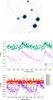 |
Fig. A.1 ASAS data of CSS J054243.2-114742 (star in the centre of the top panel) phased with elements given in VSX. The middle panel demonstrates problems caused by large aperture, the bottom panel shows confusing the target with nearby stars in different fields (blocks of data). |
An additional problem caused by close stars could arise from the combination of different fields. The bottom panel of Fig. A.1
shows the measurements in aperture 1 for different blocks of the data set. It is apparent that in different fields (blocks 3, 5, 7) the variable star was mistaken for one of the close nonvariable stars. Only blocks 2 and 9 probably show the data for the target star exclusively.
Appendix B: Additional tables and figures
Known BL stars where we did not detect the modulation.
Stars in which we cannot find any sign of variability or detect any period.
Stars with duplicate occurrence in VSX (the same coordinates and pulsation properties).
Known BL stars from literature detected in our ASAS sample.
Stars of different variability type originally classified as RRab stars in VSX.
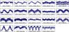 |
Fig. B.1 Stars misclassified as RRab stars in VSX identified in our sample. Data are phased with periods from Table B.5. The scales of axes are the same as in Fig. 3. |
All Tables
Stars with duplicate occurrence in VSX (the same coordinates and pulsation properties).
Stars of different variability type originally classified as RRab stars in VSX.
All Figures
|
Fig. 1 Typical ASAS data demonstrated on V1124 Her. Panels a) and b) show the data distribution and data phased with the basic pulsation period. Panel c) shows corresponding frequency spectrum; panel d) shows the spectral window. |
| In the text | |
|
Fig. 2 Typical frequency spectra after prewhitening with the basic pulsation components for BL stars, PC, and candidate stars (from left to the right). The position of the basic pulsation frequency is shown with the red dashed line. |
| In the text | |
|
Fig. 3 BL stars phased with modulation periods from Table 1. As the zero epoch we simply took HJD of the brightest data point. Ticks at the ordinate show interval of 0.2 mag, at abscissa the interval is 0.5 in BL phase. |
| In the text | |
|
Fig. 4 Magnitude distribution of all sample stars (blue) and BL stars (green grid). The distribution of modulated stars was enlarged five times for better visibility. |
| In the text | |
|
Fig. 5 BL period as a function of the pulsation period for known and new modulated stars (top), and corresponding density plot (bottom). The bottom part of the top panel shows the distribution of pulsation periods. |
| In the text | |
|
Fig. 6 Distribution of modulation periods (left-hand panel) and cumulative distribution functions (right-hand panel). It is apparent that the overall distribution follows the log-normal distribution. The agreement with the normal distribution for stars with modulation periods between 0 and 400 days shown in the insert in the right-hand panel is very good. |
| In the text | |
|
Fig. 7 Stars originally classified as pure PC. There are stars from our sample in the top panels. The middle panels show OGLE-III data demonstrating that in long-enough data sets (original classification comes from OGLE-II data with three-times shorter time span) the stars could be classified as BL stars, not pure PC stars. The bottom panels show two stars that clearly show amplitude modulation with periods shorter than 2/3TS suggesting classification as BL+PC, not pure PC. The scales of the axes are the same as in Fig. 3. |
| In the text | |
|
Fig. A.1 ASAS data of CSS J054243.2-114742 (star in the centre of the top panel) phased with elements given in VSX. The middle panel demonstrates problems caused by large aperture, the bottom panel shows confusing the target with nearby stars in different fields (blocks of data). |
| In the text | |
|
Fig. B.1 Stars misclassified as RRab stars in VSX identified in our sample. Data are phased with periods from Table B.5. The scales of axes are the same as in Fig. 3. |
| In the text | |
Current usage metrics show cumulative count of Article Views (full-text article views including HTML views, PDF and ePub downloads, according to the available data) and Abstracts Views on Vision4Press platform.
Data correspond to usage on the plateform after 2015. The current usage metrics is available 48-96 hours after online publication and is updated daily on week days.
Initial download of the metrics may take a while.