| Issue |
A&A
Volume 592, August 2016
|
|
|---|---|---|
| Article Number | A137 | |
| Number of page(s) | 12 | |
| Section | The Sun | |
| DOI | https://doi.org/10.1051/0004-6361/201628753 | |
| Published online | 15 August 2016 | |
Mapping the coronal hydrogen temperature in view of the forthcoming coronagraph observations by Solar Orbiter
INAF–Catania Astrophysical Observatory, 95123 Catania, Italy
e-mail: sdo@oact.inaf.it
Received: 20 April 2016
Accepted: 17 June 2016
Context. Synergistic visible light and ultraviolet coronagraphic observations are essential to investigate the link of the Sun to the inner heliosphere through the study of the dynamic properties of the solar wind.
Aims. We perform spectroscopic mapping of the outer solar corona to constitute a statistically significant database of neutral hydrogen coronal temperatures, which is suitable for overcoming the lack of spectrometric information in observations performed by coronagraphs that are solely equipped for visible light and ultraviolet imaging; these include the forthcoming Metis instrument on board Solar Orbiter.
Methods. We systematically analysed neutral hydrogen Lyα line data that was obtained by UVCS/SOHO observations of the extended solar corona relevant to a lot of polar, mid-latitude and equatorial structures at different phases of solar activity, and collected far longer than a whole solar cycle (1996−2012).
Results. We created a database consisting in both the neutral hydrogen temperature components, which are perpendicular and parallel to the radially symmetric coronal magnetic field lines, as a function of the heliocentric distance and polar angle and for different phases of the solar activity cycle. We validated the reliability of the constituted neutral hydrogen temperature database, investigating a new set of UVCS Lyα data with the Doppler dimming technique. The solar wind outflow velocities obtained by adopting both the neutral hydrogen temperature distribution directly derived from the observed Lyα profiles and those taken from our database well agree within the uncertainties.
Key words: Sun: corona / solar wind / Sun: UV radiation
© ESO, 2016
1. Introduction
Space observations show that the energy created in the interior of the Sun is transported into the solar corona and, by the solar wind, into the heliosphere. This wide region surrounding the Sun extends beyond the orbit of the farthest planets of the solar system and also influences the terrestrial environment. Scientists investigate the link of the Sun to the inner heliosphere through the study of the dynamic properties of the solar wind. However, the insufficient instrumental observational capabilities of the missions to the Sun have not yet allowed full exploration of the connection region between coronal solar wind and heliospheric structures, despite improvements in knowledge of the mechanisms governing the solar corona.
The Solar Orbiter mission (Müller et al. 2013) was selected by the European Space Agency (ESA) in October 2011 and scheduled for the launch in October 2018. It has the aim of studying the mechanisms through which the Sun creates and controls the heliosphere, exploring the Sun-heliosphere connection via an innovative suite of compact in situ and remote-sensing instruments, and a new orbital approach. The Metis coronagraph (Antonucci et al. 2012) was selected to be part of Solar Orbiter scientific payload. Metis will provide off-limb and near-Sun simultaneous imaging of the solar corona from 1.6 to 9 R⊙ in polarized visible light (VL) and in the H i Lyα ultraviolet (UV) line, with the aim of contributing to address the scientific goals of the Solar Orbiter mission. Specifically, it will study the origin and acceleration of the fast and slow solar wind and the origin and early propagation of coronal mass ejections (CMEs). It will benefit from the heritage of knowledge of the basic properties of coronal structures that has been enriched in recent decades thanks to the science performed by coronagraphs and spectrometers, such as the UltraViolet Coronagraph Spectrometer (UVCS; Kohl et al. 1995) onboard the SOlar and Heliospheric Observatory (SOHO; Domingo et al. 1995).
Synergistic VL coronagraphic and UV spectroscopic observations are essential to determine the fundamental physical and dynamical conditions of the solar corona. The electron density of the coronal plasma can be deduced from the VL coronagraphy, while the temperature distributions of the emitting neutral or ionized atoms from UV spectroscopy. The knowledge of these physical parameters is, in turn, central to diagnose the solar wind velocity through the Doppler dimming technique (Hyder & Lytes 1970; Noci et al. 1987; Withbroe et al. 1982), which exploits the intensity reduction occurring in the emission of coronal UV lines from regions with solar wind outflows. Therefore, knowledge of the neutral hydrogen temperature distribution is an important pre-requirement to derive detailed information about the solar wind outflow via the analysis of the coronal H i Lyα UV line.
Observation log for UVCS data.
Knowledge of characteristic temperature distributions of the neutral H i atoms obtained for a large sample of coronal structures observed at different phases of the solar cycle could be an useful support to the diagnostics of coronal structures when observed by coronagraphic instrumentations that are only equipped for imaging. So far, coronal H i temperature distributions have been derived by UVCS/SOHO observations in the Lyα line only for some selected coronal structures (see e.g. Dolei et al. 2015; Spadaro et al. 2007; Susino et al. 2008), despite the huge amount of the Lyα data obtained by UVCS. The aim of this work is to exploit all the potential of the UVCS Lyα database by systematically analysing the observations referring to a lot of polar, mid-latitude and equatorial structures at different phases of the solar activity. The results will provide for the first time a global mapping of the neutral hydrogen temperature in the whole solar corona, and ultimately a reliable and statistically significant database of H i coronal temperatures. It is worth specifying that the large bulk of UVCS data, collected far longer than a whole solar cycle (1996−2012), is fundamental to construct a complete and representative database for the H i temperature in any coronal structure. In particular, our outcome should provide an useful contribution in view of the near future perspective of the Metis instrument.
2. Observations and data reduction
We use a large amount of UVCS data collected by the H i Lyα spectrometer channel, centred at 121.6 nm, to construct an extensive set of H i temperatures referring to different coronal regions as a function of polar angle (PA, measured counterclockwise from the solar north pole), heliocentric distance, and phase of solar activity cycle. Our aim is to be able to assign, on a statistical bases, a suitable range of reliable temperature values to the neutral hydrogen atoms in different coronal structures (polar holes, mid-latitude features, and equatorial streamers), to be adopted when spectrometric observations are not available. In Table 1 we list the UVCS datasets that have been used in this work. Each observation has been catalogued on the basis of solar activity phase, year, observational time, and nominal position (expressed in PA) of the UVCS entrance slit centre.
The 360 detector pixels sampled by the UVCS entrance slit cover 42 arcmin on the plane of the sky of the spectrometer, i.e. 7 arcsec per pixel, corresponding to about 0.007 R⊙. On-board masking combines adiacent spatial pixels for increasing the signal-to-noise ratio. We perform a further binning for always making the fitting process of the observed line successful. Each final bin corresponds to the average over groups of ten combined pixels of the UVCS detector and is located at the centre of each group.
We adopt the last version of the Data Analysis and processing Software (DAS 5.1; developed by C. Benna, A. Van Ballegoijen, J. Raymond, and S. Giordano) for flat-field correction and for wavelength and radiometric calibration. In particular, the line-fitting routine sulfit.pro1, written for Interactive Data Language (IDL) environment, was used to automatically estimate and remove the stray light contribution, as well as that from the interplanetary Lyα line, to the coronal H i Lyα line emission. Subtraction of the background and instrumental line broadening correction was also performed before determining line intensities and widths (Kohl et al. 1997).
The Doppler broadening of the observed Lyα line profile includes both thermal and non-thermal components along the line of sight (LOS), such as wave or turbulent motions, and possible contribution from solar wind expansion. Therefore, the Lyα line width, derived from the spectrometric observations, provides only an upper limit of the H i temperature component in the direction of the observer and perpendicular to the magnetic field lines (T⊥), when a radially symmetric coronal magnetic field is assumed. The temperature component parallel to the magnetic field lines (T∥), which is important for a proper analysis of the Doppler dimming effect (see e.g. Cranmer et al. 1999), is then determined from T⊥ under suitable assumptions, as described in Sect. 3.
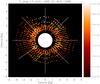 |
Fig. 1 Map of H i temperature perpendicular to the magnetic field lines obtained by the UVCS observations from August 13, 1996 to August 31, 1996. The colour bar indicates the temperature range in Kelvin. The white solid lines indicate the positions of the axes of the eight angular sectors, as described in the text. |
We use the T⊥ values obtained by the analysis of the Lyα line widths to perform an evaluation of the coronal temperature as a function of the heliocentric distance, polar angle, and solar activity phase, taking into account all the datasets listed in Table 1. As an example, Fig. 1 shows a map of T⊥ values obtained by the UVCS data reduction. Each points in the map represents the final bin and reports the temperature values averaged over the time interval from August 13, 1996 to August 31, 1996. The T⊥ values range between 4.5 × 10⁵ K and 3.4 × 10⁶ K. These boundary temperatures refer to equatorial and polar regions, respectively. For the sake of simplicity, we consider the whole corona as subdivided into eight angular sectors, which are 20 degrees wide and whose axes are separated by 45 degrees, starting counterclockwise from the north pole (0° PA). The white solid lines in Fig. 1 denote the positions of the axes of such angular sectors. To carry out the evaluation of the H i coronal temperature, we finally average the T⊥ values referring to all the bins located at the same heliocentric distance within each coronal sector. Figures 2−4 show the mean T⊥ values resulting for the eight angular sectors and for the different phases of the solar activity cycle. Symbols in the plots refer to the datasets reported in Table 1, as indicated in the common legend. Data related to observations carried out during intermediate phases of activity are all shown in Fig. 3, putting together increasing and declining phases because no substantial variation was found. The black solid lines represent the fits of the mean T⊥ values obtained for all the datasets within each angular sector. We use the functional form given by Vasquez et al. (2003), 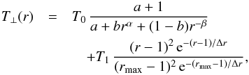 (1)where r is the heliocentric distance, Δr and rmax are the range and the maximum value of coronal heights observed by UVCS, respectively, and a, b, α, β, T0, and T1 are free parameters, whose initial estimates are reported in Table 1 of Vasquez et al. (2003). These authors used Eq. (1) to describe the perpendicular temperature of the solar wind protons, however, the rapid charge exchange between protons and neutral hydrogen atoms, especially at lower altitudes, makes their temperature distributions very similar (Withbroe et al. 1982). In particular, Allen et al. (1998) found that the H i distribution reflects the proton distribution at radii up to about 3 R⊙ in the polar regions and even higher in the equatorial regions, whereas above 3 R⊙ in the polar regions the two temperature distributions differ by about 20% at most (see e.g. Olsen & Leer 1996; Olsen et al. 1994).
The decrease of the coronal density with height reduces the rate of collisions between protons and H i atoms, which progressively decouple. In addition, the decreasing density causes a depletion of the coronal Lyα emission, which could become significantly less intense than the corresponding emission of the interplanetary plasma, which is characterized by H i temperature distributions of the order of 104 K (Bertaux et al. 1997). All this might explain the observed narrowing of the H i Lyα profile at higher altitudes, which was already noticed by some authors (see e.g. Suleiman et al. 1999; Susino et al. 2008). This occurrence appears in the trend of the temperature with height, especially in the polar regions during the minimum of the solar cycle. In this activity phase, the polar coronal holes are very large and high-latitude observations at r> 1.5R⊙ are almost unaffected by streamers. Figure 2 shows that the H i temperature in the coronal holes increases by about 1 MK from 1.5 R⊙ to 3–3.5 R⊙, corresponding to an increase of the H i Lyα line width with the height (see e.g. Antonucci et al. 2000; Kohl et al. 1997; Nakagawa 2008). Above these altitudes the temperature values become either nearly constant or slightly decreasing with height, as shown in the plots related to observations at 0° and 180° PA. In the equatorial regions (see plots at 90° and 270° PA), the H i temperature keeps around 1.4–2.0 MK at every height, with a slightly decreasing trend, similar to that found by Dolei et al. (2015), Strachan et al. (2002), and Vasquez et al. (2003). Conversely, the behaviour at mid-latitude does not exhibit a unique and definite trend.
This scenario changes during the intermediate and maximum phases of the solar cycle. The streamer structures spread in the solar corona and measurements of H i temperature give similar dependences on height even at different latitudes. Figures 3 and 4 mostly show that the temperature increases at lower altitudes and decreases above 2 R⊙ (see e.g. Miralles 2005; Spadaro et al. 2007; Susino et al. 2008). We note that UVCS data obtained by observations carried out during the maximum phase at 90° and 135° PA are very scanty and all below 2.5 R⊙. Fitting these data provides poorly reliable information about H i temperatures at higher altitudes.
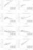 |
Fig. 2 Measurements of H i temperature perpendicular to the magnetic field lines as a function of the heliocentric distance, obtained by analysing observations carried out during the minimum phase of the solar activity cycle. Plots show the results at the different angular sectors separated by 45 degrees counterclockwise from the solar north pole (0° PA). The solid black lines represent the fits of the data, according to the functional form given by Eq. (1). |
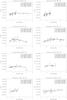 |
Fig. 3 As in Fig. 2, but for observations carried out during the intermediate phases of the solar activity cycle, considering together both increasing phase and declining phase. |
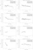 |
Fig. 4 As in Fig. 2, but for observations carried out during the maximum phase of the solar activity cycle. |
3. H I temperature anisotropy
The UVCS observations of heavier ions, such as O VI, show that their temperature distributions are anisotropic: the T⊥ values derived from the observed line profiles are higher than the T∥ values determined consistently with the Doppler dimming analysis. In particular, in polar coronal holes Telloni et al. (2007) found strong evidence of O VI anisotropic conditions between 2.0 and 3.7 R⊙. In this range of heliocentric distances the anisotropy ratio T⊥/T∥ reaches its maximum of about 14 at 2.9 R⊙ and further out approaches isotropy at about 3.7 R⊙. Based on solar minimum observations of streamers, Frazin et al. (2003) found strong anisotropic conditions for the O VI ions in streamer legs and stalk at heights above 2.3 R⊙. Conversely, isotropic temperature distribution is found in the streamer core. This last result is also supported by the investigation of Strachan et al. (2002).
A similar behaviour, even if with a lower degree, has been found for the neutral hydrogen temperature (see e.g. Cranmer et al. 1999; Spadaro et al. 2007). This condition can be formally described by a bi-Maxwellian distribution with two different temperature components T⊥ and T∥ (see details in Allen et al. 1998) for the emitting particles moving along directions perpendicular and parallel to the magnetic field lines, respectively. Cranmer et al. (1999) studied the emission of the H i Lyα line measured by UVCS in coronal polar regions during the solar minimum. They modelled the line intensity and profile shape through the Doppler dimming technique, by assuming two models for the H i temperature implying both isotropic (Maxwellian distribution) and anisotropic (bi-Maxwellian distribution) conditions. The authors found that the most consistent solutions of their models are anisotropic, with T⊥>T∥, since a larger T∥ would not be consistent with the mass flux conservation. Their results, in terms of ratio T⊥/T∥, are reported in Fig. 5 as a function of the heliocentric distance. More recently Spadaro et al. (2007) determined the physical parameters of a mid-latitude streamer during the declining phase of the solar cycle. They used a bi-Maxwellian distribution for the emitting ions in the Doppler dimming computation and found that the component of the H i temperature parallel to the magnetic field results in a factor of 1.3 smaller than the respective perpendicular component, independent of height (see Fig. 5).
The study of the dynamic properties of the solar wind requires complete knowledge of the neutral hydrogen temperature distribution and, hence, of its perpendicular and parallel components. We derive the H i temperature component T∥ starting from the T⊥ values obtained by the fitting procedure discussed in Sect. 2, and properly adopting the values of anisotropy found by Cranmer et al. (1999) and Spadaro et al. (2007). The results are shown in Figs. 6−8 as a function of the heliocentric distance. The plots refer to different polar angles and phases of the solar activity cycle, and still consider both the increasing and declining activity phase together. The feasible values of T∥ (shaded area) range between the conditions of maximum anisotropy (T⊥>T∥, red line) and isotropy (T⊥ = T∥, blue line). We assume two different trends for the anisotropy in mid-latitude regions, depending on the phase of solar activity; during the minimum, we adopt the values derived for coronal holes, owing to their large latitudinal extent in this phase of the cycle, whereas we adopt the values found for streamers in the intermediate and maximum phases.
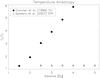 |
Fig. 5 H i temperature anisotropy in terms of the T⊥/T∥ ratio for coronal holes (CH, dots) and streamers (STR, triangles). |
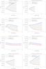 |
Fig. 6 H i temperature parallel to the magnetic field lines as a function of the heliocentric distance derived from measurements of T⊥ during the minimum phase of the solar activity cycle. Plots show the results at the different angular sectors separated by 45 degrees counterclockwise from the solar north pole (0° PA). The range of feasible T∥ values (shaded area) is delimited by the conditions of maximum anisotropy (red line) and isotropy (blue line). |
 |
Fig. 7 As in Fig. 6, but for observations carried out during the intermediate phases of the solar activity cycle, considering both increasing phase and declining phase together. |
 |
Fig. 8 As in Fig. 6, but for observations carried out during the maximum phase of the solar activity cycle. |
4. Doppler dimming analysis of outflow velocities in coronal structures
Solar wind outflow velocity.
The values of T⊥ as a function of the heliocentric distance, obtained by the fitting procedure, and those of T∥, computed as described above, build up the database of neutral hydrogen coronal temperatures. This is the main goal of the present work, however, our data archive will only turn out to be really significant if it is possible to prove its reliability for overcoming the lack of essential spectrometric information in observations performed by coronagraphs that are solely equipped for imaging. This will be the case, for instance, for the forthcoming Metis coronagraph on board Solar Orbiter.
We investigate this aspect by first selecting UVCS observations that are different from those quoted in Table 1 and used in the construction of the H i temperature database. In particular, the new datasets refer to radial scans of coronal streamers and coronal holes at different polar angles that are carried out during different solar cycle phases (see Table 2). For each observation, we derive the H i outflow velocities by adopting the Doppler dimming technique. This method requires previous knowledge of physical quantities, such as the coronal electron density and temperature and the H i temperature, which can be derived by VL coronagraphic data and UV spectrometric measurements.
We use polarized brightness images of the LASCO C2 coronagraph on board SOHO satellite (calibrated by the standard routinereduce_level_1.pro for IDL) and determine radial profiles of the coronal electron density by means of the Van De Hulst inversion technique (Billings 1966; Van De Hulst 1950) in the hypothesis of cyndrical symmetry (see e.g. Dolei et al. 2015; Hayes et al. 2001). We then derive the coronal electron temperatures starting from the electron density values and under the assumption of hydrostatic equilibrium (see e.g. Dolei et al. 2015; Gibson et al. 1999). This assumption can be reasonably applied when the outflow speed is well below the sound speed (about 150 km s-1 for a coronal plasma at 1 MK, see e.g. Priest 1987). Hence the equilibrium only holds in the equatorial and mid-latitude regions and in polar regions below 2.5 R⊙. In all of the other cases, the values of electron temperature are only a first approximation estimate, however,the temperatures found by the adopted assumption are consistent with those reported in the literature (see e.g. Fineschi et al. 1998). The values of electron temperature are then used to determine the neutral hydrogen fraction, which is necessary to derive the H i outflow velocity through the Doppler dimming effect.
In addition, the UVCS/SOHO observations provide us an evaluation of the coronal Lyα line intensity and an estimate of the H i temperature from the analysis of Lyα line profiles. We apply the Doppler dimming technique and, assuming isotropic H i temperature distribution (T⊥ = T∥), use both the T⊥ values obtained by the UVCS measurements and those catalogued in the constructed database, referring to the specific structure, solar cycle phase, polar angle, and heliocentric distance.
The proper determination of the coronal outflow velocity vw ultimately allows us to theoretically reproduce the Lyα line intensities measured by UVCS as closely as possible (see e.g. Dolei et al. 2015; Susino et al. 2008). Table 2 shows the resulting outflow speeds with their corresponding uncertainties. The fifth column reports the velocities obtained by adopting the T⊥ values derived from the UVCS spectrometric observations. The sixth column reports the velocities obtained by assuming the T⊥ values derived for similar structures via the fitting procedure described in Sect. 2; these are part of our database. The results are in a very good agreement, within the uncertainties, and this well supports the possibility of reasonably employing the data archive for scientific applications in future observations. The UVCS data related to observations performed during the maximum phase of the solar activity have not been considered in the comparison analysis owing to the lack of useful UVCS observations in the field of view covered by LASCO C2 and the consequent impossibility of applying the Doppler dimming technique.
We also carried out the computation of the outflow velocities in the coronal structures investigated during the observations reported in Table 2 under conditions of maximum anisotropy (T∥ given by the red line in Figs. 6−8), by adopting the values of T⊥ and T∥ of the constructed data archive. The last column of Table 2 shows the results of this further analysis. The differences between these outflow velocities and those computed in the case of isotropic H i temperature distribution (sixth column of Table 2) are all within the estimated uncertainties. In addition, we note opposite trends for high and low speed regimes. This is not surprising on the basis of the results reported and widely discussed in Dolei et al. (2015), who investigated the dependence of the Lyα scattering process on the temperature of the emitting atoms. The mean temperature of the neutral hydrogen atoms THI can be expressed in terms of T⊥ and T∥ as THI = (T∥ + 2 T⊥) / 3 (see e.g. Allen et al. 2000). Then, the H i mean temperature is lower in anisotropic conditions (T⊥>T∥) than in the isotropic case (T⊥ = T∥). As reported in Dolei et al. (2015), a lower temperature induces an increase for low speeds and a decrease for high speeds of the scattered Lyα line intensity, with the transition between the two regimes occurring at about 130 km s-1 (see Fig. 14 in Dolei et al. 2015). As a consequence, to properly fit the observed Lyα line intensities, the outflow velocities computed in maximum anisotropic conditions are systematically lower in fast solar wind regions (5° and 353° PA in Table 2) and systematically higher in regions of low outflow speeds (51° PA in Table 2) than the corresponding values computed in the isotropic case. The very low degree of anisotropy characterizing the streamer core regions (see Fig. 5), in nearly static conditions, accounts for the unchanged results obtained at 90° PA.
In general, our results are also consistent with outflow velocities for plasma ejected from sources of fast and slow solar wind. The low density plasma regions, such as the polar coronal holes, present values of fast outflows for neutral hydrogen atoms, which range between 130 and 250 km s-1 for distances from 2.5 to 3.5 R⊙ (see e.g. Cranmer 2002). Conversely, the high density coronal structures at lower latitudes give rise to slow outflow speeds, of the order of 50 km s-1 at about 4 R⊙, with almost static conditions at lower altitudes; these were found, for instance by Susino et al. (2008), who studied the physical properties of a mid-latitude quiescent streamer visible on May 2004, and by Dolei et al. (2015), who investigated the characteristics of an equatorial streamer during the most recent solar minimum.
5. Summary and conclusions
We systematically analysed H i Lyα data obtained by UVCS observations of the extended solar corona, relevant to a lot of polar, mid-latitude, and equatorial structures at different phases of the solar activity. Our purpose is to provide a global map of the neutral hydrogen temperature in the whole corona, and ultimately a reliable and statistically significant database of the H i coronal temperatures. A high percentage of the available observations collected near the minimum and maximum of solar activity was analysed, while those considered for intermediate periods represent well the observations carried out during those activity phases. Hence we have a good coverage of the entire set of UVCS data, collected far longer than a whole solar cycle (1996−2012).
For each coronal region examined, we derived the upper limits of the H i temperature component in the direction of the observer by the measurements of the Lyα line width. This component is also perpendicular to the magnetic field lines, assuming a radially symmetric coronal magnetic field, and usually defined as T⊥. The temperature component parallel to the magnetic field lines, T∥, was then determined from the T⊥ values, both in the case of isotropic temperature distribution (T⊥ = T∥) and assuming different levels of anisotropy (T⊥>T∥) found in the scientific literature.
All the values of T⊥, obtained by the analysis of the Lyα line widths, and of T∥, determined as described above, constitute an extended database of neutral hydrogen coronal temperatures. This is suitable for overcoming the lack of essential spectrometric information in observations performed by coronagraphs that are solely equipped for VL and UV imaging, such as the forthcoming Metis instrument on board Solar Orbiter. The knowledge of both components of the neutral hydrogen temperature distribution is crucial for the study of the dynamics properties of the solar wind, in particular for the diagnostics of the wind outflow velocity through the Doppler dimming technique (Hyder & Lytes 1970; Noci et al. 1987; Withbroe et al. 1982).
Finally, we proved the reliability of the temperature database considering other sets of UVCS Lyα data, which are different from those taken into account for constructing our database, and relevant to radial scans of coronal streamers and coronal holes at different polar angles that were carried out during different solar cycle phases. The values of solar wind outflow velocity resulting from the Doppler dimming analysis of the new sets of data, which adopt both the H i temperatures directly derived by the spectroscopic analysis of the observed Lyα profiles and those taken from our database, are in a very good agreement within the uncertainties. This fully supports the possibility of reasonably employing the data archive built in the present work for scientific applications in future Lyα observations of the solar outer corona.
Available from the Harvard-Smithsonian Center for Astrophysics website: cfa-www.harvard.edu/uvcs
Acknowledgments
The authors wish to thank the Principal Investigator, Ester Antonucci, and all the team of the Metis coronagraph for Solar Orbiter, for suggesting this investigation. They also thank the referee for his/her helpful comments and the Italian Space Agency (ASI) for partially supporting this work through contract ASI/INAF No. I/013/12/0.
References
- Allen, L. A., Habbal, S. R., & Hu, Y. Q. 1998, J. Geophys. Res., 103, 6551 [Google Scholar]
- Allen, L. A., Habbal, S. R., & Li, X. 2000, J. Geophys. Res., 105, 23123 [NASA ADS] [CrossRef] [Google Scholar]
- Antonucci, E., Dodero, M. A., & Giordano, S. 2000, Sol. Phys., 197, 115 [NASA ADS] [CrossRef] [Google Scholar]
- Antonucci, E., Fineschi, S., Naletto, G., et al. 2012, SPIE, 8443, 9 [Google Scholar]
- Bertaux, J. L., Quémerais, E., Lallement, R., et al. 1997, Sol. Phys., 175, 737 [NASA ADS] [CrossRef] [Google Scholar]
- Billings, D. E. 1966, A guide to the Solar Corona (New York: Academic Press) [Google Scholar]
- Cranmer, S. R. 2002, Space Sci. Rev., 101, 229 [Google Scholar]
- Cranmer, S. R., Kohl, J. L., Noci, G., et al. 1999, ApJ, 511, 481 [NASA ADS] [CrossRef] [Google Scholar]
- Dolei, S., Spadaro, D., & Ventura, R. 2015, A&A, 577, A34 [NASA ADS] [CrossRef] [EDP Sciences] [Google Scholar]
- Domingo, V., Fleck, B., & Poland, A. I. 1995, Sol. Phys., 162, 1 [NASA ADS] [CrossRef] [Google Scholar]
- Fineschi, S., Gardner, L. D., Kohl, J. L., Romoli, M., & Noci, G. C. 1998, SPIE, 3443, 67 [Google Scholar]
- Frazin, R. A., Cranmer, S. R., & Kohl, J. L. 2003, ApJ, 597, 1145 [NASA ADS] [CrossRef] [Google Scholar]
- Gibson, S. E., Fludra, A., Bagenal, F., et al. 1999, J. Geophys. Res., 104, 9691 [NASA ADS] [CrossRef] [Google Scholar]
- Hayes, A. P., Vourlidas, A., & Howard, R. A. 2001, ApJ, 548, 1081 [NASA ADS] [CrossRef] [Google Scholar]
- Hyder, C. L., & Lytes, B. W. 1970, Sol. Phys., 14, 147 [NASA ADS] [Google Scholar]
- Kohl, J. L., Esser, R., Gardner, L. D., et al. 1995, Sol. Phys., 162, 313 [NASA ADS] [CrossRef] [Google Scholar]
- Kohl, J. L., Noci, G., Antonucci, E., et al. 1997, Sol. Phys., 175, 613 [NASA ADS] [CrossRef] [Google Scholar]
- Miralles, M. P. 2005, IAGA, 10, 79 [Google Scholar]
- Müller, D., Marsden, R. G., St. Cyr, O. C., & Gilbert, H. R. 2013, Sol. Phys., 285, 25 [NASA ADS] [CrossRef] [Google Scholar]
- Nakagawa, A. 2008, ApJ, 674, 1167 [NASA ADS] [CrossRef] [Google Scholar]
- Noci, G., Kohl, J. L., & Withbroe, G. L. 1987, ApJ, 315, 706 [NASA ADS] [CrossRef] [Google Scholar]
- Olsen, E. L., & Leer, E. 1996, ApJ, 462, 982 [NASA ADS] [CrossRef] [Google Scholar]
- Olsen, E. L., Leer, E., & Holzer, T. 1994, ApJ, 420, 913 [NASA ADS] [CrossRef] [Google Scholar]
- Priest, E. R. 1987, Solar Magneto-Hydrodynamics (Dordrecht: Reidel Publ. Co.) [Google Scholar]
- Spadaro, D., Susino, R., Ventura, R., Vourlidas, A., & Landi, E. 2007, A&A, 475, 707 [NASA ADS] [CrossRef] [EDP Sciences] [Google Scholar]
- Strachan, L., Suleiman, R., Panasyuk, A. V., Biesecker, D. A., & Kohl, J. L. 2002, ApJ, 571, 1008 [Google Scholar]
- Suleiman, R. M., Kohl, J. L., Panasyuk, A. V., et al. 1999, Space Sci. Rev., 87, 327 [NASA ADS] [CrossRef] [Google Scholar]
- Susino, R., Ventura, R., Spadaro, D., Vourlidas, A., & Landi, E. 2008, A&A, 488, 303 [NASA ADS] [CrossRef] [EDP Sciences] [Google Scholar]
- Telloni, D., Antonucci, E., & Dodero, M. A. 2007, A&A, 476, 1341 [NASA ADS] [CrossRef] [EDP Sciences] [Google Scholar]
- Van De Hulst, H. C. 1950, Bull. Astron. Inst. Netherland, 410, 135 [Google Scholar]
- Vasquez, A. M., Van Ballegooijen, A. A., & Raymond, J. C. 2003, ApJ, 598, 1361 [NASA ADS] [CrossRef] [Google Scholar]
- Withbroe, G. L., Kohl, J. L., Weiser, H., & Munro, R. H. 1982, Space Sci. Rev., 33, 17 [NASA ADS] [CrossRef] [Google Scholar]
All Tables
All Figures
|
Fig. 1 Map of H i temperature perpendicular to the magnetic field lines obtained by the UVCS observations from August 13, 1996 to August 31, 1996. The colour bar indicates the temperature range in Kelvin. The white solid lines indicate the positions of the axes of the eight angular sectors, as described in the text. |
| In the text | |
|
Fig. 2 Measurements of H i temperature perpendicular to the magnetic field lines as a function of the heliocentric distance, obtained by analysing observations carried out during the minimum phase of the solar activity cycle. Plots show the results at the different angular sectors separated by 45 degrees counterclockwise from the solar north pole (0° PA). The solid black lines represent the fits of the data, according to the functional form given by Eq. (1). |
| In the text | |
|
Fig. 3 As in Fig. 2, but for observations carried out during the intermediate phases of the solar activity cycle, considering together both increasing phase and declining phase. |
| In the text | |
|
Fig. 4 As in Fig. 2, but for observations carried out during the maximum phase of the solar activity cycle. |
| In the text | |
|
Fig. 5 H i temperature anisotropy in terms of the T⊥/T∥ ratio for coronal holes (CH, dots) and streamers (STR, triangles). |
| In the text | |
|
Fig. 6 H i temperature parallel to the magnetic field lines as a function of the heliocentric distance derived from measurements of T⊥ during the minimum phase of the solar activity cycle. Plots show the results at the different angular sectors separated by 45 degrees counterclockwise from the solar north pole (0° PA). The range of feasible T∥ values (shaded area) is delimited by the conditions of maximum anisotropy (red line) and isotropy (blue line). |
| In the text | |
|
Fig. 7 As in Fig. 6, but for observations carried out during the intermediate phases of the solar activity cycle, considering both increasing phase and declining phase together. |
| In the text | |
|
Fig. 8 As in Fig. 6, but for observations carried out during the maximum phase of the solar activity cycle. |
| In the text | |
Current usage metrics show cumulative count of Article Views (full-text article views including HTML views, PDF and ePub downloads, according to the available data) and Abstracts Views on Vision4Press platform.
Data correspond to usage on the plateform after 2015. The current usage metrics is available 48-96 hours after online publication and is updated daily on week days.
Initial download of the metrics may take a while.