| Issue |
A&A
Volume 592, August 2016
|
|
|---|---|---|
| Article Number | A160 | |
| Number of page(s) | 8 | |
| Section | The Sun | |
| DOI | https://doi.org/10.1051/0004-6361/201628335 | |
| Published online | 24 August 2016 | |
Properties of sunspot cycles and hemispheric wings since the 19th century
1 ReSoLVE Centre of Excellence, Space
Climate Research Unit, University of Oulu, 90017
Oulu,
Finland
e-mail: This email address is being protected from spambots. You need JavaScript enabled to view it.
2 Sodankylä Geophysical Observatory
(Oulu unit), University of Oulu, 90017
Oulu,
Finland
3 Leibniz Institute for Astrophysics
Potsdam, 14482
Potsdam,
Germany
Received:
18
February
2016
Accepted:
17
June
2016
Abstract
Aims. The latitudinal evolution of sunspot emergence over the course of the solar cycle, the so-called butterfly diagram, is a fundamental property of the solar dynamo. Here we present a study of the butterfly diagram of sunspot group occurrence for cycles 7–10 and 11–23 using data from a recently digitized sunspot drawings by Samuel Heinrich Schwabe in 1825–1867, and from RGO/USAF/NOAA(SOON) compilation of sunspot groups in 1874–2015.
Methods. We developed a new, robust method of hemispheric wing separation based on an analysis of long gaps in sunspot group occurrence in different latitude bands. The method makes it possible to ascribe each sunspot group to a certain wing (solar cycle and hemisphere), and separate the old and new cycle during their overlap. This allows for an improved study of solar cycles compared to the common way of separating the cycles.
Results. We separated each hemispheric wing of the butterfly diagram and analysed them with respect to the number of groups appearing in each wing, their lengths, hemispheric differences, and overlaps.
Conclusions. The overlaps of successive wings were found to be systematically longer in the northern hemisphere for cycles 7–10, but in the southern hemisphere for cycles 16–22. The occurrence of sunspot groups depicts a systematic long-term variation between the two hemispheres. During Schwabe time, the hemispheric asymmetry was north-dominated during cycle 9 and south-dominated during cycle 10.
Key words: Sun: activity / sunspots
© ESO, 2016
1. Introduction
Detailed information on sunspot locations has recently been obtained for the early past by digitizing and analysing historical sunspot drawings (Hoyt & Schatten 1992; Vaquero 2007; Arlt 2008, 2009a,b, 2011; Vaquero et al. 2011; Carrasco et al. 2013; Casas & Vaquero 2014). This makes it possible to study, for example, the time-latitude occurrence of sunspots, such as the Maunder butterfly diagram, much further back into the past than was possible earlier.
Although the level of solar activity is readily apparent from the amount of sunspots or sunspot groups, the sunspot numbers do not contain all information on the nature of the sunspot cycle. Carrington (1858) first noted that the sunspots appear on average at lower latitudes during times of decreasing activity, and start appearing on two separate belts at high latitudes of the two hemispheres, as the activity begins to rise, with a varying degree of overlap between the high and low latitude belts of sunspot activity. This latitudinal evolution of sunspot occurrence was presented by Maunder (1904) in a diagram in which the latitudes of sunspots are presented as a function of time.
The magnetic nature of the sunspot cycle became apparent after Hale et al. (1919) discovered the change of sunspot polarity from one cycle to another. This led to the conclusion that the 11-year Schwabe cycle is actually only half of the 22-year magnetic Hale sunspot cycle. After an activity minimum, the sunspots appearing on the higher latitude belts have oppositely ordered magnetic polarity compared to those (of the previous cycle) at lower latitude. As the cycle progresses, the mean latitude of sunspot occurrence starts migrating towards the solar equator until they are confined to latitudes of about ± 10°−15° close to the end of the cycle, however leaving a zone of avoidance near the equator. Differences between solar hemispheres have been reported in numerous publications since the study by Spoerer (1889, 1890), who noted that, during some periods of the sunspot cycle, sunspots occur only within one hemisphere.
In this paper we discuss the sunspot butterfly diagram, which is separated into individual hemispheric shapes commonly referred to as wings. The beginning of a new cycle wing and the end of an old cycle wing usually overlap in time by a few years around the cycle minimum, leading to a superposition of the two wings (and cycles) around the minimum. Analysing separate wings makes it possible to study the so-called extended cycles (Wilson et al. 1988; Usoskin & Mursula 2003; Cliver 2014), the latitudinal evolution of sunspots, the hemispheric differences and other surface phenomena produced by the solar dynamo. We study the sunspot groups and determine, for instance, the length and overall group activity of each wing separately. We also study the hemispheric asymmetry of wings, which is often known to be significant and to produce fairly systematic phenomena (see e.g. Newton & Milsom 1955; Carbonell et al. 1993; Verma 1993; Pulkkinen et al. 1999; Li et al. 2002; Mursula & Hiltula 2003; Ballester et al. 2005; Virtanen & Mursula 2010, 2014).
This paper is organized as follows. In Sect. 2 we describe the data sets used in this study. Section 3 defines the maxima, minima, and other details of the sunspot cycles. Section 4 describes the method to separate the hemispheric wings in the butterfly diagram and Sect. 5 presents several characteristic values of the wings and the hemispheric differences of wings. In Sect. 6 we give our conclusions.
2. Data
The Royal Greenwich Observatory – USAF/NOAA(SOON) sunspot data set (referred here as RGO data) contains information on sunspot group locations and areas since 1874. This series may be affected by uneven quality before 1900 (Clette et al. 2014; Willis et al. 2016) but it still remains the only centennial series with location and area information of sunspot groups extending until present. The recently digitized observations of Samuel Heinrich Schwabe (Arlt 2011; Arlt et al. 2013) provide an extension of this data set to the years 1825–1867, covering solar cycles 7–10. This data set contains a wide potential for analysis since it also lists the locations and sizes of individual sunspots. In particular, the latitudinal evolution of sunspots gives vital information for studies on the long-term operation of the solar dynamo, where the polarity of magnetic fields on the Sun is not known.
The Schwabe data contains information on individual sunspots in contrast to the sunspot group data of the RGO record. From the Schwabe data we used information on sunspot latitudes in addition to the number of sunspots and sunspot groups. A typical drawing from Schwabe’s notebooks is shown in Fig. 1. A detailed assessment on the observations and their quality is given by Arlt (2011) and Arlt et al. (2013) The data set1 was subject to several revisions since its first publication, and for this study we used the version 1.2 of 5.12.2014. Since the groups defined by Schwabe are not fully consistent with the modern understanding, the sunspot groups have been redefined. The fraction of revisited sunspot groups in the total number of sunspot groups is on average less than 10% in the first half of observations, but can be up to 35% in the second half. A detailed description of the group definition and the homogeneity of the data set is given elsewhere by Senthamizh Pavai et al. (2015). They noted that the change in the spots-per-group ratio around 1835–1836 might be due to a combined effect of a change in drawing style around 1830–1831, and the solar minimum in 1833, since an increase in the number of spots per group can be seen after other minima as well.
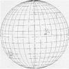 |
Fig. 1 Typical drawing from Schwabe’s notebooks along with the overlaid heliographic coordinate system. This particular image illustrates the transition from cycle 9 to cycle 10 showing both a low-latitude and a high-latitude group. |
The RGO data 2 was used for the time period of 1874–2015. This data set is actually a compilation of data from different observatories. The Royal Greenwich Observatory compilation covers the years 1874–1976. For the data between 1977−2015, when the sunspot data was produced by the US Air Force and National Oceanic and Atmospheric Administration (USAF/NOAA), we applied the correction factor 0.65 (cf. Hathaway 2010). This factor was applied to the monthly mean number of groups. Since the RGO data set does not contain information on individual sunspots, but only lists the mean latitudes and total sizes covered by sunspot groups, we calculated a similar set from the Schwabe data to be better comparable with the RGO data. The ensuing Schwabe sunspot group data set contains a list of all sunspot groups for each day and their mean latitudes; we do not weight the latitude by spot areas here. The two data sets are, however, not straightforwardly comparable for all of their properties, including the total activity level, because of the differences in, for example observation techniques and, in particular, because of the different coverages of observation time.
3. Sunspot cycle characteristics
The Wolf sunspot number (WSN) was developed by Wolf (1861) who combined sunspot observations from several observers into a single series of sunspot numbers. For a given time period he used observations of a primary observer whenever they were available. Otherwise he used observations made by a secondary or tertiary observer. Wolf allocated an individual scaling factor for each observer according to their level of experience and equipment. Note that the adopted linear scaling is not an appropriate way to calibrate observers (Lockwood et al. 2016; Usoskin et al. 2016). The Wolf sunspot number for a given day is calculated as 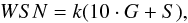 (1)where G is the number of sunspot groups, S is the number of individual sunspots, and k is the observer’s scaling factor. Schwabe was the primary observer for Wolf sunspot numbers for the period 1825–1848 with a scaling factor of 1.25. As we have shown earlier (Leussu et al. 2013), however, this scaling factor was overestimated by about 20%. This is why for our calculations we set k = 1 for Schwabe. The Schwabe data does, however, contain a lower sunspot count in the early part of the data in relation to group counts, implying that the scaling factor overestimate is valid only for the later part of Schwabe’s observations. The entire sunspot number data has recently been revised3 (cf. Clette et al. 2014), but this revision has been subject to some debate (e.g. Lockwood et al. 2016; Usoskin et al. 2016).
Hoyt & Schatten (1998) introduced another index of solar activity, the group sunspot number (GSN). It is more robust since sunspot groups are more easily observable than individual spots (Usoskin 2013). The GSN series is available for a longer period of time than the WSN. The daily value for the group sunspot number is calculated as 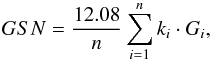 (2)where n is the number of observers whose observations were used for a particular day, Gi is the number of sunspot groups as reported by ith observer, ki is the individual scaling factor of the observer, and the factor 12.08 is used to normalize the GSN to the level of WSN in 1874–1976 (Hoyt & Schatten 1998). Similar to WSN, for our calculations we use ki = 1 for the Schwabe data. Since GSN takes all available observations of sunspot groups by all observers into account, it is less prone to errors arising, for instance from wrongly assigned individual scaling factors than WSN (Especially for the primary observer; Leussu et al. 2013). However, the exact scaling factor 12.08 has recently been questioned because of an inhomogeneity within the RGO data between 1874–1885 (Cliver & Ling 2016; Willis et al. 2016). Therefore, we drop the factor 12.08 from our calculations and use an unscaled measure for sunspot group numbers.
We study the properties of sunspot cycles from the Schwabe data using both the Wolf (WSN-S) and Group (GSN-S) sunspot numbers based solely on Schwabe’s drawings. The series are smoothed with the 13-month Gleissberg filter (GF) so that the smoothed monthly mean  for month k is calculated as
  (3)where Ri indicates the monthly mean of any sunspot number series. Such smoothing is a common method to define the dates of maxima and minima of the sunspot cycle (see e.g. Mursula & Ulich 1998; Hathaway 2010). A more sophisticated approach to a smoothed monthly mean addressing the uneven number of observing days per month would involve Monte Carlo simulations (which goes beyond the scope of this paper), but adopting this approach is not expected to greatly alter the results obtained in this paper. The GF filtered monthly averaged WSN-S and GSN-S series are presented in Fig. 2. With the scaling coefficient 12.08, the ratio between WSN-S and GSN-S should be unity throughout the whole series, but it in fact increases above one in the rising phase of cycle 8. This increase is probably related to the sudden increase in spots/group ratio in Schwabe data in 1836 (Senthamizh Pavai et al. 2015). The difference between WSN-S and GSN-S over most of the Schwabe time interval indicates a change in the relative normalization of WSN and GSN between the Schwabe data and the sunspot series in the 20th century, which was used to normalize the GSN to WSN. This difference is not due to the redefinition of Schwabe group numbers, since roughly the same difference was found earlier using Schwabe’s original group numbering (Leussu et al. 2013). Also using the scaling factor 1.25 denoted by Wolf for Schwabe would further increase this difference; a variable WSN/GSN ratio during the 20th century has recently been noted by Clette et al. (2014).
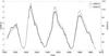 |
Fig. 2 Gleissberg-filtered monthly WSN-S (grey) and GSN-S (black) calculated from the Schwabe data. |
3.1. Sunspot cycle maxima
First we define the dates of sunspot cycle maxima for Schwabe data. We determine these dates from: (1) maxima of the GF-smoothed WSN-S series and (2) maxima of the GF-smoothed GSN-S series. The corresponding dates and maximum values are listed in Table 1. We also included in Table 1 the dates and values of sunspot maxima determined by Waldmeier (1961). When calculating the times of maxima, Waldmeier considered the monthly mean sunspot numbers and the number of sunspot groups in addition to the GF-smoothed monthly mean sunspot numbers (Hathaway 2010). This is probably the reason for the differences in the dates for maxima of cycles 7−9 in Table 1. The three dates agree with each other only for cycle 10. Also, Waldmeier always gave the earliest date for the maxima. The WSN-S maximum values differ, roughly by a factor of 1.2 from the values listed by Waldmeier (1961), mainly because of the scaling factor discussed above. The maximum values of WSN-S and GSN-S are close to each other when brought to the same scale for cycle 7, but differ for cycles 8−10 (WSN higher than GSN), in agreement with above discussion.
Dates and values for sunspot cycle maxima from the GF-smoothed WSN-S and GSN-S series along with the dates and values given by Waldmeier (1961).
3.2. Sunspot cycle minima
Determining the minimum times is not straightforward. Even during sunspot minima the Sun exhibits weak, variable sunspot activity, making the concept of a minimum rather complicated. Determining the dates for sunspot cycle minima is complicated if, for instance there is a long time period of no activity or several separate periods of roughly equally low (or no) activity during the same extended minimum. Hathaway (2010) gives a detailed account on the cycle minimum times determined by considering several aspects of sunspot activity: smoothing of sunspot numbers, monthly fraction of spotless days, and the number of old cycle groups versus new cycle groups. Although the physical significance of the notion of a sunspot minimum can be somewhat vague, we consider it here for a direct comparison with earlier studies.
The monthly fraction of spotless days is calculated as the ratio between observed spotless days within a month and the total number of observations during that month, which corresponds to the mathematical expectation even in the case of fractional coverage. Observing the fraction of spotless days in his early observations actually led Schwabe to the discovery of the sunspot cycle (Schwabe 1844). A smoothed monthly fraction of spotless days for the Schwabe data is shown in Fig. 3. The smoothed monthly fraction Fk for month k was calculated by the formula  (4)where Sk is the number of spotless days in month k, and Nk is the total number of observations in month k.
The dates for the cycle minima were determined by three methods: (1) minima of the GF-smoothed WSN-S series; (2) minima of the GF-smoothed GSN-S series; and (3) maxima in the smoothed monthly fraction of spotless days (SD). These values are collected in Table 2 together with dates given by Waldmeier (1961). The dates obtained using all three methods are very close to each other and agree for all but one of the three full minima (7/8). The Waldmeier date coincides with that given by the maximum in the spotless days fraction for this minimum.
Dates for the sunspot minima obtained from the GF-smoothed WSN-S and GSN-S series and from the fraction of spotless days (SD), along with the dates given by Waldmeier (1961).
Table 3 shows the lengths for sunspot cycles 8–10 calculated from the minimum dates in Table 2 for all four methods. The length of cycle 7 is only a lower limit and the length of cycle 10 may also be slightly longer than given in Table 3. The length estimates for cycles 8 and 10 agree very closely between the four methods and match exactly for cycle 9. Waldmeier and the spotless days method give the same lengths for the two definitely defined cycles 8–9. We note the large difference of about 2.5−3 yrs between cycles 8 and 9, although their amplitudes do not differ significantly.
4. Separating butterfly wings
An analysis based solely on sunspot numbers does not contain full information on magnetic activity or hemispheric differences, since the old and new cycle usually overlap in time, making the sunspot number at sunspot minimum a superposition of the old and new cycles. Definite separation of the new and old cycle spots can best be done using the magnetic polarity of the sunspots. If, however, the information on magnetic polarity is not available, as is the case with the Schwabe data, the separation of wings of the butterfly diagram can be made based on the latitude information of sunspots or sunspot groups.
Here we introduce a method to separate two consecutive sunspot wings by defining a borderline consisting of two linear segments in the butterfly diagram. The two segments are defined by spotless gaps between the two wings, in a way described below; the gaps can also include breaks in observation in addition to spotless days.
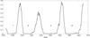 |
Fig. 3 Smoothed monthly fraction of spotless days. |
First we divided the whole data set into latitude belts with a width of 2°. These latitude bands were then searched for long gaps between any two successive sunspot groups. We took into account each occurrence of a sunspot group on all days this group was observed, which naturally emphasizes groups with longer lifetime, i.e. mostly large groups. Different threshold (minimum) gap lengths were used for different latitude bands. The optimum threshold lengths for the gaps were determined by testing different combinations of threshold lengths for different latitudes. We tested threshold lengths from 100 to 800 days with 50 day intervals. Different thresholds for different latitudes were needed since the typical gap lengths between sunspots vary with latitude. Using threshold lengths that are too short or too long would have resulted in either outliers in sparse areas (specifically gaps that are between two sunspot groups belonging to the same wing) or not enough gaps in areas that are rather dense with sunspot groups. High latitudes, as well as the equatorial area, were studied with longer thresholds than mid-latitudes because sunspots appear more sparsely in those locations. The main criterion was to have few (preferably only one) gaps for as many latitude bands as possible.
Table 4 lists the gap threshold lengths that we finally used for the different latitude bands for Schwabe and RGO sunspot group data sets. We gathered the dates of the centres of all gaps at all latitude bands found using the threshold values into a data set in Table 4. The border segment for each pair of wings was defined by fitting a line to the set of gap centres between the equator and 28° latitude band, separately for each pair and each hemisphere. The line fit was calculated using a linear regression between gap centre times and their latitudes with a bisquare weighted robust fitting. The fitted lines were then used as borders between the wings for sunspot separation up to the latitudes of ± 28°. Beyond ± 28° the separation was carried out by a vertical line. The vertical separation at high latitudes was necessary because in some cases the continuation of the fitted line would separate the wings clearly erroneously by including a high-latitude part of the wing of the previous cycle into the next cycle.
Gap threshold lengths in days for different latitude bands of the Schwabe and RGO data sets for sunspot groups.
Figure 4 shows the separation process for the southern wings of cycles 8 and 9. The grey data points belong to the southern wing of cycle 8 and the black points to southern wing of cycle 9. The dividing (non-vertical) line is obtained by a fit to the detected gap centres, which are shown with black circles. In this case, only one latitude band included two gaps (and gap centres), and the others only included one.
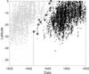 |
Fig. 4 A fragment of the butterfly diagram around the gap between the southern wings of cycles 8 and 9. Sunspot groups belonging to cycle 8 are plotted in grey and cycle 9 groups in black. The centres of all the detected gaps longer than the threshold gap length of Table 4 are plotted in black circles. The fitted line up to −28° and the vertical line poleward of −28° between the wings are plotted in black. |
Figure 5 shows the result of wing separation in the form of the butterfly diagram for both Schwabe and RGO data, indicating each wing separately by alternating colour. Each point represents a sunspot group at the group mean latitude on the day it occurred. All groups are plotted for all days they were observed, not only for the first appearance. Separating the wings based on the group data produces a more robust and clear separation than using sunspot data. Figure 5 shows some differences between Schwabe and RGO data. The wider latitudinal spread and the lack of a zone of avoidance is obvious in Schwabe data. This zone does not appear as clearly in Schwabe data, mostly because the Schwabe drawings are less accurate than the Greenwich photographs. Another prominent feature occurs because of the change in production of the data from RGO to NOAA in 1977 when the latitudes are reported with the accuracy of 1 degree instead of 0.1 degree used until then, leading to latitudinal stripes in Fig. 5. Figure 5 shows that our method gives a reasonably good separation even in cases where two consecutive wings are overlapping for a long time, as for example between cycles 8 and 9, and cycles 19–21. The method does not, however, perform well with separating the northern wings of cycles 10 and 11 because the latitude range of groups of the new cycle 11 is too small for a reliable fit. The separation, which is very clear as seen in Fig. 5, the separation was performed manually for this pair of wings. The southern wings were not changed since the method gives a plausible result.
 |
Fig. 5 Butterfly diagram after separating wings of Schwabe and RGO data. Each point represents a sunspot group plotted at the mean latitude of the sunspots belonging to that group, on every day it was observed. Different colours distinguish the two successive wings. |
5. Results
Table 5 features a collection of properties of the wings of cycles 7–10 calculated from the Schwabe data. They include the total spot and group counts, the dates for the first and last spot appearing in each wing, the maximum number of spots and groups on the most active day of the wing, and the dates and values of the maxima of GF-smoothed WSN-S and GSN-S for the separate wings. The allocation of sunspot to the wings was made based on the group to which they belong) While for all other wings (north or south) the relation between the total number of spots and groups is about 4–5, for cycle 7 wings this remains at about 2–3; this is very likely valid even if cycle 7 is not complete. This change is also related to the change in the WSN-S to GSN-S ratio during early cycle 8 as depicted in Fig. 2. Also, even though the maximum daily number of sunspots varies considerably from wing to wing, the maximum daily number of sunspot groups (8–9) remains surprisingly constant. This is another indication of the change in spots/group ratio around 1836 within Schwabe’s observations. Senthamizh Pavai et al. (2015) stated that the change is most likely because of a superposition of two effects: the change in drawing style around 1830–1831 and the recovery of solar activity from the 1833 minimum.
For cycles 8 and 9, and most likely for cycle 7, the total counts of spots and groups are considerably (20%−30%) larger in the northern than the southern hemisphere. For cycle 10 the relation is reversed and the southern hemisphere is about 10% more active than the northern hemisphere. We study this in more detail later. Wing lengths are given in Table 6 for both Schwabe and RGO data.
Properties of wings in the two hemispheres for cycles 7 and 8.
The monthly GSN-S and WSN-S for the separate wings are plotted in Figs. 6 and 7, respectively, along with the GF-smoothed monthly means; the GSN-S here is simply the monthly mean number of groups. One can see that the overlap between successive wings varies a lot from one minimum to another. While there is very little overlap (less than one year) between the wings of cycles 7 and 8, there is a very long overlap between the wings of cycles 8 and 9 with the wings of cycle 8 extending far beyond the time of the minimum. The cycle 9/10 minimum shows a similar behaviour as the cycle 8/9 minimum with a long overlap of old cycle wings extending beyond the time of minimum. The difference between the two hemispheres is most striking in the start of cycle 9, where the northern hemisphere clearly dominates in activity over the southern hemisphere.
Sums of monthly mean number of groups over the wings and lengths of wings (in years).
Figure 8 shows the absolute and relative differences between the GF-smoothed GSN-S in the northern (GSN-SN) and southern (GSN-SS) wings; the times when the GF-smoothed curve in one hemisphere is zero is not included in the differences since the relative difference would be ± 1 and distort the figure. At the minimum between cycles 8 and 9 the southern hemisphere of cycle 8 dominates, leading to negative asymmetries. This is probably the reason for the note by Zolotova et al. (2010) that the start of cycle 9 would be dominated by the southern hemisphere. In contrast to Zolotova et al. (2010), we find that the northern wing dominates over the southern wing during cycle 9. The activity of the previous cycle (9) also dominates around the next minimum between cycles 9 and 10, and the northern wing of cycle 9 dominates over the southern wing. However, the asymmetry is reversed in cycle 10, and the southern wing clearly dominates at the start of cycle 10, which is in agreement with Zolotova et al. (2010).
We also calculated wing-averaged values of the monthly mean GSN in the northern (GN) and southern (GS) wings for both the Schwabe and RGO data sets. The relative difference (GN-GS)/(GN+GS) and the absolute differences (GN-GS) are shown in Fig. 9.
The sums of the monthly mean number of groups over the wings WN and WS, along with the lengths of all (Schwabe and RGO period) wings are collected in Table 6. The lengths were calculated as the time difference between the last and first sunspot group within that wing. The overlap times of wings are listed in Table 7. The three overlaps of Schwabe time are all longer in the northern hemisphere, in agreement with the wing lengths being longer there (see Table 6). Also, during the last seven minima the overlaps are larger in the southern hemisphere, where most of the wings are also longer at this time (see Table 6). The wing lengths cannot be considered very robust, since small changes in the wing separation parameters can mislocate some sunspot groups, and the wing length can change by up to two years, however, the systematic nature of the above results suggests that they are real.
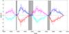 |
Fig. 6 Monthly means (thin curves) of GSN-S along with the GF-smoothed monthly means (thick curves) for separate butterfly wings. Negative values denote values for the southern hemisphere. Vertical lines denote times of minima given in Table 2. Grey areas denote wing overlap times. |
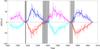 |
Fig. 7 Monthly means (thin curves) of WSN-S along with the GF-smoothed monthly means (thick curves) for separate butterfly wings. Negative values denote values for the southern hemisphere. Vertical lines denote times of minima given in Table 2. Grey areas denote wing overlap times. |
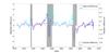 |
Fig. 8 Relative difference (cyan for cycles 7 and 9, and blue for cycles 8 and 10) and absolute difference (magenta for cycles 7 and 9 and red for cycles 8 and 10) between the GF-smoothed GSN-S in the northern wing (GSN-SN) and the southern wing (GSN-SS). Vertical lines denote times of minima based on Table 2. Grey areas denote wing overlap times. |
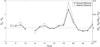 |
Fig. 9 Relative (grey; right y-axis) and absolute (black; left y-axis) difference between the wing-averaged monthly GSN in the northern wing and the southern wing for cycles 7–10 and 12–24. |
Overlap times of northern and southern wings in years.
Figure 10 shows the relative differences (WN-WS)/(WN+WS), and the absolute differences (WN-WS) between WN and WS. Both Fig. 9, which gives an estimate of the hemispheric differences in the average group activity level of the wings, and Fig. 10, which gives the same estimate for the cumulative activity levels, depict a mutually consistent behaviour. The largest positive (negative) values of the absolute and relative differences between the two hemispheres are found in sunspot cycles 19 and 20 (cycles 12 and 22) for both pairs of parameters (GN, GS and WN, WS). The difference is positive during most of the previous century and depicts negative values at the end of the 19th and 20th century, indicating a systematic long-term variation in the hemispheric asymmetry, which is in a close agreement with earlier results (Zhang et al. 2013). There is also some indication of a shorter variation of the difference at the period of about 5 cycles. Newton & Milsom (1955) studied the hemispheric asymmetry from the RGO and Schwabe data but their study was based on sunspot areas for RGO and spot counts from Schwabe; these authors concluded that a cyclic behaviour is not apparent. Pulkkinen et al. (1999) studied the long-term variation in the position of the magnetic equator and concluded that it has a variation in timescale of around 90 yrs.
Figure 11 shows the cumulative sums of the monthly mean number of sunspot groups calculated over each wing (cf. Li et al. 2001). It shows clearly that the difference in activity between the two hemispheres may remain the same sign over the whole cycle or it may change during the cycle. Cycles 9–10, 15, and 18–20 all show a similar behaviour where the stronger hemisphere is the same throughout the whole cycle. During cycle 9 the dominant hemisphere is north, as also shown in Fig. 8. The same is true for cycles 15, 19, and 20. In cycle 20 the difference between the two hemispheres is more systematic than in any other cycle, even more so than in cycle 8. We note also that both of these two cycles, 8 and 20, are the next cycles after the highest cycle of the respective century. The only cycles that are systematically south-dominated are cycle 10 (see also Fig. 8) and cycle 18. In the remaining cycles the stronger hemisphere changes at least once during the cycle.
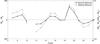 |
Fig. 10 Relative (grey; right y-axis) and absolute (black; left y-axis) difference between the sum of monthly mean number of groups in the northern wing and the southern wing for cycles 7–10 and 12–24. |
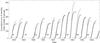 |
Fig. 11 Cumulative sum of monthly mean number of groups for the northern wings (dashed line) and southern wings (solid line). |
6. Conclusions
We have analysed a combination of two sunspot data sets with information on sunspot groups and their locations: the RGO data and Schwabe data. The RGO data only has information on sunspot groups, whereas the Schwabe data also has information on the observed individual spots. The RGO data covers the end of sunspot cycle 11, full cycles 12–23, and the beginning of the current cycle 24, whereas the Schwabe data covers most of cycle 7, full cycles 8 and 9, almost all of cycle 10, and the very beginning of the wings of the new cycle 11.
Our main findings and results obtained in the paper can be summarized as follows:
Times of sunspot cycle minima and maxima were defined anew for cycles 7–10 using different methods and compared with the conventional dates (Waldmeier 1961). All these dates are close to each other, implying that their definition is robust.
The ratio between the Wolf and group sunspot number during most of time covered by Schwabe data is higher than that derived by Hoyt & Schatten (1998). This may indicate non-uniformity of the normalization factor 12.08 in the GSN, which might have been related to an inhomogeneity in the early part of the RGO data compilation (cf. Willis et al. 2016; Cliver & Ling 2016).
We introduced a simple and robust method to separate the butterfly wings. The wings were analysed with respect to the number of groups appearing in each wing, their lengths, hemispheric differences, and overlaps.
We calculated the Wolf and group sunspot numbers for the separate wings for the original Schwabe data (cycles 7–10). While the maximum daily number of sunspots varied significantly (30–80) for different cycles, the maximum daily number of groups remained roughly the same (8–9) throughout the wings covered by the Schwabe data. This may be partly due to the lower counts of sunspots in the early part of Schwabe data.
We found that the overlaps of the hemispheric wings around the cycle minima were systematically longer in the northern hemisphere for cycles 7 through 10, while they were longer in the southern hemisphere in the last 7 solar cycle minima; this suggests long-term variability. The sunspot occurrence within the wings depicts a systematic variable long-term asymmetry between the two hemispheres.
We found that, while the hemispheric asymmetry of the wings was north dominated in the beginning of cycle 9, it was south dominated in the beginning of cycle 10. If the north-south asymmetry is related to the phase lag between the two hemispheres, the data appear to place the transition proposed by Zolotova et al. (2010) to have occurred between cycles 9 to 10.
Available at http://www.aip.de/Members/rarlt/sunspots/schwabe
Available at http://solarscience.msfc.nasa.gov/greenwch.shtml
Acknowledgments
We acknowledge the financial support by the Academy of Finland to the ReSoLVE Centre of Excellence (project No. 272157).
References
- Arlt, R. 2008, Sol. Phys., 247, 399 [NASA ADS] [CrossRef] [Google Scholar]
- Arlt, R. 2009a, Sol. Phys., 255, 143 [NASA ADS] [CrossRef] [Google Scholar]
- Arlt, R. 2009b, Astron. Nachr., 330, 311 [NASA ADS] [CrossRef] [Google Scholar]
- Arlt, R. 2011, Astron. Nachr., 332, 805 [NASA ADS] [CrossRef] [Google Scholar]
- Arlt, R., Leussu, R., Giese, N., Mursula, K., & Usoskin, I. G. 2013, MNRAS, 433, 3165 [NASA ADS] [CrossRef] [Google Scholar]
- Ballester, J. L., Oliver, R., & Carbonell, M. 2005, A&A, 431, L5 [NASA ADS] [CrossRef] [EDP Sciences] [Google Scholar]
- Carbonell, M., Oliver, R., & Ballester, J. L. 1993, A&A, 274, 497 [NASA ADS] [Google Scholar]
- Carrasco, V. M. S., Vaquero, J. M., Gallego, M. C., & Trigo, R. M. 2013, New Astron., 25, 95 [NASA ADS] [CrossRef] [Google Scholar]
- Carrington, R. C. 1858, MNRAS, 19, 1 [NASA ADS] [CrossRef] [Google Scholar]
- Casas, R., & Vaquero, J. M. 2014, Sol. Phys., 289, 79 [NASA ADS] [CrossRef] [Google Scholar]
- Clette, F., Svalgaard, L., Vaquero, J. M., & Cliver, E. W. 2014, Space Sci. Rev., 186, 35 [NASA ADS] [CrossRef] [Google Scholar]
- Cliver, E. W. 2014, Space Sci. Rev., 186, 169 [Google Scholar]
- Cliver, E. W., & Ling, A. G. 2016, Sol. Phys., in press [Google Scholar]
- Hale, G. E., Ellerman, F., Nicholson, S. B., & Joy, A. H. 1919, ApJ, 49, 153 [NASA ADS] [CrossRef] [Google Scholar]
- Hathaway, D. H. 2010, Liv. Rev. Sol. Phys., 7, 1 [Google Scholar]
- Hoyt, D. V., & Schatten, K. H. 1992, ApJS, 78, 301 [NASA ADS] [CrossRef] [Google Scholar]
- Hoyt, D. V., & Schatten, K. H. 1998, Sol. Phys., 181, 491 [NASA ADS] [CrossRef] [Google Scholar]
- Leussu, R., Usoskin, I. G., Arlt, R., & Mursula, K. 2013, A&A, 559, A28 [NASA ADS] [CrossRef] [EDP Sciences] [Google Scholar]
- Li, K. J., Yun, H. S., & Gu, X. M. 2001, ApJ, 554, L115 [NASA ADS] [CrossRef] [Google Scholar]
- Li, K. J., Wang, J. X., Xiong, S. Y., et al. 2002, A&A, 383, 648 [NASA ADS] [CrossRef] [EDP Sciences] [Google Scholar]
- Lockwood, M., Owens, M. J., Barnard, L., & Usoskin, I. G. 2016, Sol. Phys., in press [Google Scholar]
- Maunder, E. W. 1904, MNRAS, 64, 747 [NASA ADS] [Google Scholar]
- Mursula, K., & Hiltula, T. 2003, Geophys. Res. Lett., 30, 2135 [Google Scholar]
- Mursula, K., & Ulich, T. 1998, Geophys. Res. Lett., 25, 1837 [NASA ADS] [CrossRef] [Google Scholar]
- Newton, H. W., & Milsom, A. S. 1955, MNRAS, 115, 398 [NASA ADS] [CrossRef] [Google Scholar]
- Pulkkinen, P. J., Brooke, J., Pelt, J., & Tuominen, I. 1999, A&A, 341, L43 [NASA ADS] [Google Scholar]
- Schwabe, H. 1844, Astron. Nachr., 21, 233 [NASA ADS] [CrossRef] [Google Scholar]
- Senthamizh Pavai, V., Arlt, R., Dasi-Espuig, M., Krivova, N. A., & Solanki, S. K. 2015, A&A, 584, A73 [NASA ADS] [CrossRef] [EDP Sciences] [Google Scholar]
- Spoerer, F. W. G. 1890, MNRAS, 50, 251 [NASA ADS] [Google Scholar]
- Spoerer, G. 1889, Bull. Astron., Ser. I, 6, 60 [Google Scholar]
- Usoskin, I. G. 2013, Liv. Rev. Sol. Phys., 10, 1 [Google Scholar]
- Usoskin, I. G., & Mursula, K. 2003, Sol. Phys., 218, 319 [NASA ADS] [CrossRef] [Google Scholar]
- Usoskin, I. G., Kovaltsov, G. A., Lockwood, M., et al. 2016, Sol. Phys., in press [Google Scholar]
- Vaquero, J. M. 2007, Adv. Space Res., 40, 929 [Google Scholar]
- Vaquero, J. M., Gallego, M. C., Usoskin, I. G., & Kovaltsov, G. A. 2011, ApJ, 731, L24 [NASA ADS] [CrossRef] [Google Scholar]
- Verma, V. K. 1993, ApJ, 403, 797 [NASA ADS] [CrossRef] [Google Scholar]
- Virtanen, I. I., & Mursula, K. 2010, J. Geophys. Res., 115, 9110 [Google Scholar]
- Virtanen, I. I., & Mursula, K. 2014, ApJ, 781, 99 [Google Scholar]
- Waldmeier, M. 1961, The sunspot-activity in the years 1610−1960 (Verlag Schulthess) [Google Scholar]
- Willis, D. M., Wild, M. N., & Warburton, J. S. 2016, Sol. Phys., in press [Google Scholar]
- Wilson, P. R., Altrocki, R. C., Harvey, K. L., Martin, S. F., & Snodgrass, H. B. 1988, Nature, 333, 748 [NASA ADS] [CrossRef] [Google Scholar]
- Wolf, R. 1861, MNRAS, 21, 77 [NASA ADS] [Google Scholar]
- Zhang, L., Mursula, K., & Usoskin, I. 2013, A&A, 552, A84 [NASA ADS] [CrossRef] [EDP Sciences] [Google Scholar]
- Zolotova, N. V., Ponyavin, D. I., Arlt, R., & Tuominen, I. 2010, Astron. Nachr., 331, 765 [NASA ADS] [CrossRef] [Google Scholar]
All Tables
Dates and values for sunspot cycle maxima from the GF-smoothed WSN-S and GSN-S series along with the dates and values given by Waldmeier (1961).
Dates for the sunspot minima obtained from the GF-smoothed WSN-S and GSN-S series and from the fraction of spotless days (SD), along with the dates given by Waldmeier (1961).
Gap threshold lengths in days for different latitude bands of the Schwabe and RGO data sets for sunspot groups.
Sums of monthly mean number of groups over the wings and lengths of wings (in years).
All Figures
|
Fig. 1 Typical drawing from Schwabe’s notebooks along with the overlaid heliographic coordinate system. This particular image illustrates the transition from cycle 9 to cycle 10 showing both a low-latitude and a high-latitude group. |
| In the text | |
|
Fig. 2 Gleissberg-filtered monthly WSN-S (grey) and GSN-S (black) calculated from the Schwabe data. |
| In the text | |
|
Fig. 3 Smoothed monthly fraction of spotless days. |
| In the text | |
|
Fig. 4 A fragment of the butterfly diagram around the gap between the southern wings of cycles 8 and 9. Sunspot groups belonging to cycle 8 are plotted in grey and cycle 9 groups in black. The centres of all the detected gaps longer than the threshold gap length of Table 4 are plotted in black circles. The fitted line up to −28° and the vertical line poleward of −28° between the wings are plotted in black. |
| In the text | |
|
Fig. 5 Butterfly diagram after separating wings of Schwabe and RGO data. Each point represents a sunspot group plotted at the mean latitude of the sunspots belonging to that group, on every day it was observed. Different colours distinguish the two successive wings. |
| In the text | |
|
Fig. 6 Monthly means (thin curves) of GSN-S along with the GF-smoothed monthly means (thick curves) for separate butterfly wings. Negative values denote values for the southern hemisphere. Vertical lines denote times of minima given in Table 2. Grey areas denote wing overlap times. |
| In the text | |
|
Fig. 7 Monthly means (thin curves) of WSN-S along with the GF-smoothed monthly means (thick curves) for separate butterfly wings. Negative values denote values for the southern hemisphere. Vertical lines denote times of minima given in Table 2. Grey areas denote wing overlap times. |
| In the text | |
|
Fig. 8 Relative difference (cyan for cycles 7 and 9, and blue for cycles 8 and 10) and absolute difference (magenta for cycles 7 and 9 and red for cycles 8 and 10) between the GF-smoothed GSN-S in the northern wing (GSN-SN) and the southern wing (GSN-SS). Vertical lines denote times of minima based on Table 2. Grey areas denote wing overlap times. |
| In the text | |
|
Fig. 9 Relative (grey; right y-axis) and absolute (black; left y-axis) difference between the wing-averaged monthly GSN in the northern wing and the southern wing for cycles 7–10 and 12–24. |
| In the text | |
|
Fig. 10 Relative (grey; right y-axis) and absolute (black; left y-axis) difference between the sum of monthly mean number of groups in the northern wing and the southern wing for cycles 7–10 and 12–24. |
| In the text | |
|
Fig. 11 Cumulative sum of monthly mean number of groups for the northern wings (dashed line) and southern wings (solid line). |
| In the text | |
Current usage metrics show cumulative count of Article Views (full-text article views including HTML views, PDF and ePub downloads, according to the available data) and Abstracts Views on Vision4Press platform.
Data correspond to usage on the plateform after 2015. The current usage metrics is available 48-96 hours after online publication and is updated daily on week days.
Initial download of the metrics may take a while.