| Issue |
A&A
Volume 592, August 2016
|
|
|---|---|---|
| Article Number | A153 | |
| Number of page(s) | 9 | |
| Section | The Sun | |
| DOI | https://doi.org/10.1051/0004-6361/201628306 | |
| Published online | 22 August 2016 | |
Empirical mode decomposition analysis of random processes in the solar atmosphere
1 Centre for Fusion, Space and Astrophysics, Department of
Physics, University of Warwick, CV4 7AL, UK
e-mail: This email address is being protected from spambots. You need JavaScript enabled to view it.
2 School of Space Research, Kyung Hee
University, Yongin,
446-701
Gyeonggi,
Korea
3 Central Astronomical Observatory at
Pulkovo of the Russian Academy of Sciences, 196140
St Petersburg,
Russia
Received:
13
February
2016
Accepted:
10
June
2016
Abstract
Context. Coloured noisy components with a power law spectral energy distribution are often shown to appear in solar signals of various types. Such a frequency-dependent noise may indicate the operation of various randomly distributed dynamical processes in the solar atmosphere.
Aims. We develop a recipe for the correct usage of the empirical mode decomposition (EMD) technique in the presence of coloured noise, allowing for clear distinguishing between quasi-periodic oscillatory phenomena in the solar atmosphere and superimposed random background processes. For illustration, we statistically investigate extreme ultraviolet (EUV) emission intensity variations observed with SDO/AIA in the coronal (171 Å), chromospheric (304 Å), and upper photospheric (1600 Å) layers of the solar atmosphere, from a quiet sun and a sunspot umbrae region.
Methods. EMD has been used for analysis because of its adaptive nature and essential applicability to the processing non-stationary and amplitude-modulated time series. For the comparison of the results obtained with EMD, we use the Fourier transform technique as an etalon.
Results. We empirically revealed statistical properties of synthetic coloured noises in EMD, and suggested a scheme that allows for the detection of noisy components among the intrinsic modes obtained with EMD in real signals. Application of the method to the solar EUV signals showed that they indeed behave randomly and could be represented as a combination of different coloured noises characterised by a specific value of the power law indices in their spectral energy distributions. On the other hand, 3-min oscillations in the analysed sunspot were detected to have energies significantly above the corresponding noise level.
Conclusions. The correct accounting for the background frequency-dependent random processes is essential when using EMD for analysis of oscillations in the solar atmosphere. For the quiet sun region the power law index was found to increase with height above the photosphere, indicating that the higher frequency processes are trapped deeper in the quiet sun atmosphere. In contrast, lower levels of the sunspot umbrae were found to be characterised by higher values of the power law index, meaning the domination of lower frequencies deep inside the sunspot atmosphere. Comparison of the EMD results with those obtained with the Fourier transform showed good consistency, justifying the applicability of EMD.
Key words: Sun: atmosphere / Sun: photosphere / Sun: chromosphere / Sun: corona / sunspots / methods: data analysis
© ESO, 2016
1. Introduction
The solar atmosphere evidently shows a wide range of periodicities detected throughout the whole electromagnetic spectrum. They have different physical nature and causes, and their periods vary from a fraction of second up to several years, and even to centuries. Some examples of the oscillatory processes responsible for the periodicities are the 11 yr solar cycle, the so-called quasi-biennial oscillations, the helioseismic variations (see Hathaway 2010; Bazilevskaya et al. 2014; Christensen-Dalsgaard 2002, and references therein for recent comprehensive reviews), magnetohydrodynamic waves and oscillations in different plasma structures of the solar atmosphere (see De Moortel & Nakariakov 2012; Liu & Ofman 2014; Jess et al. 2015), and various quasi-periodic pulsations (QPP) appearing in solar flare light curves (Nakariakov & Melnikov 2009; Kupriyanova et al. 2010; Simões et al. 2015).
In addition to clear oscillations, broadband modes usually associated with noise often appear in solar signals of various types too. These noisy components may have basically different physical nature, for example, they can be caused by instrumental artefacts or by random processes operating in the solar atmosphere. Interestingly, in the majority of previous studies these modes were usually ignored and simply disregarded in analysis. However, recent works have shown that coloured noises can be recognised in solar and stellar flare light curves with the Fourier power spectrum, and accumulate a significant part of a signal’s spectral energy. They are manifested as a power-law-like Fourier power spectra, and seem to be intrinsic features of many observational data sets detected by different instruments. For example, Inglis et al. (2015) considered flare signals exhibiting QPP detected with the PROBA2 (Large Yield Radiometer), Fermi (Gamma-ray Burst Monitor), Nobeyama Radioheliograph, and Yohkoh (HXT) instruments. They found that the majority of cases considered could be described by a power law in the Fourier power spectra. Signatures of strong noisy components having power-law-like Fourier power spectral densities were also detected in Gruber et al. (2011), where the RHESSI and Fermi (Gamma-ray Burst Monitor) observations of solar flares were considered. Application of the wavelet transform modulus maxima method showed the multifractal spectra of the temporal variation of the X-ray emission in solar flares (McAteer et al. 2007).
The interest in the coloured noise in the solar atmosphere is connected with its possible link with various dynamical phenomena. For example, in the case of QPP in flares a frequency-dependent noise may be associated with repetitive magnetic reconnection (e.g. Bárta et al. 2011). In the case of the quiet Sun, the evolution of the noise with height may reveal the physical processes responsible for the generation, dissipation and evolution of magnetohydrodynamic waves, turbulence, and episodic energy releases. Recently, Ireland et al. (2015) studied mean Fourier spectra of various regions of the solar corona observed at the 171 Å and 193 Å wavelengths, and found that they can be described by a power law at lower frequencies, tailing to a flat spectrum at higher frequencies, plus a Gaussian-shaped contribution specific for different regions of the corona. Also, understanding of the noise is important for the development of automated detection techniques (e.g. Nakariakov & King 2007; Sych et al. 2010; Ireland et al. 2010; Martens et al. 2012).
In addition to the Fourier and wavelet techniques, another spectral method being actively used for the analysis of solar signals is the Hilbert-Huang Transform technique developed in Huang et al. (1998), Huang & Wu (2008). It is based upon the empirical mode decomposition (EMD) of the signal of interest into the basis derived directly from the data by iterative searching for the local time scale naturally appearing in the signal. Being not restricted by an a priori assignment of the basis function, EMD operates adaptively and, hence, is essentially suitable for processing non-stationary and non-linear time series typical for the solar signals. These unique properties of EMD attracted a growing interest in the application of this technique to analysis of dynamical phenomena on the Sun. This technique has already been successfully applied to solar signals. For example, anharmonic and multi-modal structures of solar QPP were revealed with EMD in Nakariakov et al. (2010), Kolotkov et al. (2015b), detailed two-dimensional information about a propagating and a standing wave in a coronal loop was obtained with EMD in Terradas et al. (2004), periodicities associated with the 11 yr solar cycle were investigated with EMD in Kolotkov et al. (2015a), Vecchio et al. (2012), Zolotova & Ponyavin (2007), including revealing the periodicities in the variation of the solar radius (Qu et al. 2015). Also, periodicity in the monthly occurrence numbers and monthly mean energy of coronal mass ejections was studied with EMD by Gao et al. (2012). Long-term variability of the coronal index was analysed with EMD in Deng et al. (2015). We would like to point out that a similar technique was independently designed by Nagovitsyn (1997), who applied it to the analysis of non-linear processes in the solar activity on large time scales.
In contrast to the Fourier and wavelet spectral methods, behaviour of coloured noises with arbitrary indices in power law dependences of their power spectral densities in the EMD analysis has not been clearly revealed yet. The analysis has been restricted to the EMD of a white noise (Wu & Huang 2004). Based on the empirical fact that EMD effectively operates as a dyadic filter (Flandrin et al. 2004), numerical experiments in Wu & Huang (2004) showed that intrinsic mode functions (IMF) obtained with EMD from a number of independent white noise samples are normally distributed, and the product of the IMF energy density and its mean period is constant. Furthermore, the energy density function was found to be chi-squared distributed. Analysis of a particular case of the red noise in EMD has been made in Franzke (2009), revealing noise-like properties of the Earth’s climate data.
In this paper we extend the studies of Wu & Huang (2004) and Franzke (2009), and reveal similar empirical properties of coloured noises in EMD, allowing for arbitrary indices in power law dependences of their power spectral densities in application to the solar atmosphere. We show that coloured noises can be successfully described by the chi-squared distribution too. However the parameter of the distribution function, the number of degrees of freedom (DoF), needs to be adjusted accordingly for each sort of noise. For illustration of the reliability of the method, we adapt this EMD-based technique for analysing solar extreme ultraviolet (EUV) data sets obtained with SDO/AIA, testing them in the manner described above for the presence of randomly distributed dynamical processes. Historically, observations of the oscillatory processes in the atmosphere of the Sun attract a great interest among the research community. In particular, the high-frequency tails of solar dynamical spectra, obtained from the lower layers of the solar atmosphere, were found to vary significantly with the height and magnetic properties of the region (see, e.g. Evans et al. 1963; Orrall 1966; Woods & Cram 1981; Deubner & Fleck 1990). In this paper we use the data obtained with the modern SDO/AIA instrument. Due to the advanced combination of this data’s spatial and temporal resolutions and high values of the signal-to-noise ratio, it allows us to investigate the higher coronal altitudes of the solar atmosphere in the EUV band and directly compare their dynamical spectra with the chromospheric and photospheric layers. We show that application of this EMD-based noise-test to SDO/AIA data sets revealed that they mainly consist of random signals represented by a combination of the white noise at shorter-period spectral components and the reddish noises at longer periods.
2. Methodology and properties of coloured noises in EMD
Power spectral density S of coloured noises as a function of frequency, f can be written as S = C/fα, where C is a constant which can be reduced to unity by appropriate normalisation without loss of generality, and α is a power law index characterising the steepness of the dependence, that is its “colour”. In further analysis, we consider only non-negative values of α. We recall that noises with α = 0 are usually referred to as the white noises with constant spectral energy for all considered frequencies, while non-zero values of α correspond to the so-called coloured noises. In particular, α = 1 describes a flicker (pink) noise, while α = 2 gives a Brown(ian) (red) noise.
Wu & Huang (2004) analysed behaviour of the white noise with α = 0 in EMD. Based on the numerical examples they established an empirical relation for the energy densities Em of each separate intrinsic mode function (IMF) obtained with the EMD expansion of the white noise samples and their corresponding mean periods Pm as EmPm = const. This empirical fact is directly related to the dyadic property of EMD. We note that the dyadic nature of EMD in turn may be corrupted by the so-called mode-leakage (also often referred to as mixing) problem (see, e.g. Wu & Huang 2009) causing remarkable deviations of the energy-period dependence of some particular IMF from the expected form. Additionally, the probability density function of each IMF was found to be normally distributed. The latter property leads to the chi-squared distribution of the IMF energy density Em with k degrees of freedom (DoF):  (1)By definition, the white noise of length N contains N independent and random data points. Hence, each sample of such a white noise has its N DoF which are evenly distributed across the Fourier power spectrum. As the white noise spectral energy is also evenly distributed across the spectrum, the number k in the chi-squared distribution of Em is proposed to be proportional to the mean modal energy, that is
  , where
  with n being a sufficiently large number of the white noise samples considered.
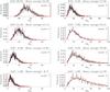 |
Fig. 1 Histograms (black) showing the normalised modal energy NEm fitted by distribution (5) (red) for several IMFs obtained with EMD from 2000 independent samples of the synthetic white (α = 0, left column) and coloured (α = 1.5, right column) noises. Each noise sample contains N = 500 data points. All samples were normalised for their total energy to be unity. |
However, this simple rule should not work for coloured noises in the case with α ≠ 0. Indeed, the spectral energy of coloured noises is distributed across the spectrum by the power law dependence mentioned above. Hence, data points of coloured noises are no longer independent, but instead they are correlated with each other. The latter makes the exact determination of the DoF number of the coloured noise, and consequently the DoF number of IMF obtained from such a noise with EMD, to be a non-trivial task. However, assuming again that the coloured noise IMFs are normally distributed, the modal energy Em can be represented by a sum of k independent normal variables Xi with zero mean and variance σ, as  (2)In the case of white noises, where the modal energies and the number of DoF are evenly distributed across the spectrum, the variance σ is of the same value for all IMFs. Hence, it can be normalised to unity, and the modal energy (2) is distributed by the chi-squared law (1) with k being the number of DoF (Wu & Huang 2004). In contrast, in the coloured noise case the number of DoF of a separate IMF may differ from the mean modal energy, and the corresponding normalisation is impossible. In this case, the quantity distributed by the chi-squared law is
  (3)with arbitrary values of σ, that in general may be different for different IMF. Using the fact that the mean value of Y is equal to the number of DoF, k, one can obtain from Eqs. (2) and (3) the value of σ of coloured noise IMFs as
  (4)Substituting Eqs. (2) and (4) into Eq. (3), we are able to write the probability density function of coloured noise IMFs energies Em in a general form as
 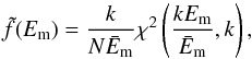 (5)which is, in fact, the chi-squared distribution of the quantity
  , governed by a single parameter k being the number of DoF, and reducing to the corresponding white noise distribution (1) for .
From a practical point of view, distribution (5) can be represented by functions E± giving its upper (99%) and lower (1%) confidence intervals, respectively. To obtain their dependences on the instant period P, E±(P), we empirically determine dependences k(P) (DoF) and  (mean modal energy density) from numerical experiments and substitute them in distribution (5). More specifically, Fig. 1 shows several examples of the modal energy NEm distribution of the synthetic noisy signals with α = 0 (white noise) and α = 1.5 (reddish noise), fitted by the probability density function (5) with DoF determined from the best fitting and the mean energy taken from the input data. The functional form of distribution (5) has been fitted to the binned histograms shown in Fig. 1 with the number of bins being 200. The fitting procedure is robust, giving identical results in a broad rang of the number of bins tested, from 20 to 1000.
The mean modal energy  of the white noise IMFs was found to change proportionally to the best fitted DoF (see Eq. (1)). However, in some cases the detected values of DoF may significantly differ from the mean modal energy. It also confirms the only approximate dyadic nature of EMD, with possible discrepancies caused by the mode-leakage problem. In contrast, the reddish noise with α = 1.5 shows rather more complicated behaviour with inverse proportionality. For both noises DoF are found to decrease with the IMF number. Additionally, for both noises, IMFs with higher values of DoF show distributions of NEm closer to the normal distribution, which is also a typical feature of the chi-squared distribution.
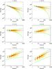 |
Fig. 2 Energy-period distributions (yellow dots) of IMFs obtained with EMD from 2000 independent samples of synthetic noisy signals with α = 0 (the white noise), α = 0.5, α = 1 (flicker or the pink noise), α = 1.5, α = 2 (Brown(ian) or the red noise), and α = 2.5. Each sample contains 500 data points. All samples were normalised for their total energy to be unity. Period is measured in dimensionless evenly sampled time-steps between the data points. The energy averaged over each period is indicated by the red crosses. Blue lines represent the empirical dependence of the mean modal energy |

The dependence is obtained by fitting the modal energy values averaged over each considered period with a linear function in a logarithmic scale (see Fig. 2). This also allows for empirical determination of the α index in the dependence S = 1 /fα. Indeed, assuming again the dyadic properties of EMD, we can calculate the energy density Em of the mth mode as: 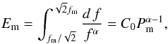 (6)where C0 is some constant, and fm and Pm are the modal frequency and period, respectively, with
  . Hence, according to Eq. (6), the empirical relation EmPm = const. obtained for the white noise (α = 0) in Wu & Huang (2004) can be generalised to the form
  (7)for coloured noises with arbitrary values of α. Similar relation between modal energies and periods has been shown in Franzke (2009). However, this study was restricted to a particular case of the red noise only. In a logarithmic scale, the slope of the line given by a y = (α − 1)x + b function with y = ln Em, x = ln Pm, and b = ln C0, allows for the estimation of the empirical value of α, appearing in the analysed sample. Numerical experiments performed with the use of synthetic signals showed that such an empirical estimation gives values of α with relative errors of up to 3.3%. We recall that the dyadic nature of EMD can still be significantly corrupted by the mode-leakage problem. Following Wu & Huang (2004) we excluded the first IMF (with the shortest period) out of fitting as it demonstrates rather different behaviour than the other modes. We also do not fit the periods that are longer than a half-length of the analysed signal as the corresponding IMFs contain insufficient number of extrema for the correct determination of their periods.
Substituting the empirical dependences k(P) and to the chi-squared distribution given by expression (5) we calculate the corresponding confidence intervals E±(P). Figure 2 shows the energy-period dependences of different modes and corresponding confidence intervals obtained empirically with the method described above for the noises with α = 0 (the white noise), α = 0.5, α = 1 (flicker or the pink noise), α = 1.5, α = 2 (Brown(ian) or the red noise), and α = 2.5. The dependences are given by the dots showing the energy and mean period of each IMF. The corresponding modal energy and mean period were calculated as  and Pm = 2N/bm, respectively, with Cm being the mth IMF, N is the total length of the signal, and bm is the number of extrema in the mth IMF. The dots are seen to scatter within the confidence intervals and are clustered together in separate groups indicating localisation of periods and energies of IMFs. In particular, numerical results obtained for the white noise samples are in consistence with those shown in Wu & Huang (2004). In Fig. 2 we also show their confidence intervals obtained with the second-order Taylor expansion of the exact dependences, and hence valid only in the regions with small deviations of Em from the mean value.
In the case when one tests some real signals for randomly distributed processes with an a priori unknown value of α, the analysis can be itemised in the following steps:
-
Normalisation of all analysed samples for their total energy beingunity before the EMD processing.
-
Empirical estimation of the power law index α from the slope of the linear fitting of the modal energy averaged over each period.
-
Construction of corresponding empirical dependencies
in form (7) and k(P) for the normalised synthetic coloured noise with a certain value of α determined above. -
Calculation of the confidence intervals E±(P) from the chi-squared distribution shown in Eq. (5) for the chosen sort of the coloured noise.
Having obtained E±(P), one can consider IMFs with an energy-period distribution within this interval to be related to a random process with a certain value of the power law index α.
3. Noise-testing of SDO/AIA data
We applied the methodology described in the previous section to the investigation of statistical properties of the EUV emission coming from the NOAA 11131 active region and its neighbourhood. We used SDO/AIA observations corresponding to different levels of the solar atmosphere: the upper photosphere (1600 Å), chromosphere (304 Å), and corona (171 Å). For each wavelength we analysed a continuous sequence of 500 images with the highest available cadence (12 s for 304 and 171 Å, and 24 s for 1600 Å) starting on 8 December 2010, 00:00:00 UT, when the active region was close to the central meridian. There were no flares during the observation. We downloaded the images from the SDO data processing centre1. Before downloading, the images were cropped, de-rotated, and coaligned.
For investigating statistical properties of the intensity variations in different channels, we selected two square regions of interest (ROI 1 and 2) shown in Fig. 3. Each ROI is of 50 pixels wide, giving us 2500 different intensity signals coming from individual pixels. The first ROI is located in the quiet sun region eastwards from the NOAA 11131 (heliographic coordinates: Θ = 29.23°, Φ = −17.46°). We placed the second ROI at the centre of the sunspot located in NOAA 11131 active region (heliographic coordinates: Θ = 31.27°, Φ = −3.98°). This sunspot showed well pronounced 3-min oscillations which were previously detected with SDO/AIA (Reznikova et al. 2012; Sych & Nakariakov 2014; Yuan et al. 2014; Deres & Anfinogentov 2015).
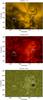 |
Fig. 3 Active region NOAA 11131 observed with SDO/AIA at the 171 Å (top), 304 Å (middle), and 1600 Å (bottom) wavelengths. Images are taken at 00:00:00 UT, 8 December 2010. White squares show the regions of interest (ROI) for intensity variations considered in this paper. |
Following the method described above we empirically found that the intensity variations of the emission coming from each individual pixel of the quiet sun region, ROI 1, have coloured noise-like behaviour with the modal energy-period dependence in the form given by Eq. (7) (see Fig. 4). Therefore we consider these intensity variation signals as random processes with a power law spectral energy distribution. The specific value of the power law index α was empirically estimated for each wavelength in the same manner that had been used for the synthetic noises (see Fig. 2), that is by the linear fitting of the average energies to the dependence (7) in a logarithmic scale. The period ranges where the fittings were carried out, were chosen to correspond to the power-law-like parts of the spectra. The value of α was found to increase with height in ROI 1 from 0.86 ± 0.03 for the upper photosphere, 1600 Å line, to 1.29 ± 0.02 for the chromosphere, 304 Å, and 1.32 ± 0.04 for the coronal 171 Å line, with corresponding 1σ uncertainties. Such a behaviour of α indicates that a higher-frequency oscillations are trapped deeper in the quiet sun atmosphere. In contrast, the intensity signals coming from the sunspot umbrae (ROI 2, see Fig. 5) in addition to a power-law-like spectral energy distribution, were found to contain several IMFs with periods of approximately two to four minutes and with energies significantly above the noise level. The latter groups of IMFs could be clearly associated with 3-min oscillations already found in this sunspot. The value of α estimated with the EMD-testing of the intensity signals coming from ROI 2 was found to decrease with height from 1.33 ± 0.04 for the upper photosphere (1600 Å), to 1.23 ± 0.1 for the chromosphere (304 Å), and 1.26 ± 0.13 for the corona (171 Å), with corresponding 1σ uncertainties, i.e. lower-frequency processes dominate at lower levels of the sunspot atmosphere. Interestingly, that the 171 Å and 304 Å intensity signals coming from ROIs 1 and 2 have nearly the same values of α, of about 1.2−1.3 corresponding to the reddish noise behaviour. On the other hand it changes dramatically for the 1600 Å line from about 0.86 in ROI 1 to 1.33 in ROI 2, indicating the change in the noise colour from the pink (flicker) to the reddish one at lower altitudes of the solar atmosphere when transiting from the quiet sun regions to the sunspot umbrae. Figures 4 and 5 also show the mean Fourier spectra for the same observational data sets, allowing for comparison of the results obtained with these two essentially different spectral techniques. Each mean Fourier spectrum was obtained by averaging of the spectra of separate signals from each individual pixel of ROIs 1 and 2. Similarly to the energy-period dependences of IMFs obtained with EMD, the mean Fourier spectra are also seen to have clear power-law-like regions at longer periods. The values of α detected with the mean Fourier spectra were found to be fully consistent with the corresponding values detected with the EMD-based testing.
More specifically, the top panels of Fig. 4 show the energy-period dependences of IMFs of the intensity variations from the quiet sun region (ROI 1), which look similarly at the 171 Å and 304 Å wavelengths. In analogy with the examples of synthetic noises shown in Fig. 2, the dependences are shown by the dots clustered in groups corresponding to separate IMFs. The spectral energy distributions have non-trivial structures and can be described as a superposition of two random processes with different power law indexes α for both 171 Å and 304 Å observational wavelengths. Indeed, at short periods (approximately shorter than two minutes) the process with α ≈ 0 (the white noise) dominates. The second component, with α being of about 1.32 and 1.29 for 171 Å and 304 Å, respectively (the reddish noise), dominates at longer periods. These two noisy components could originate from different sources and hence belong to different physical processes of a natural or instrumental origin.
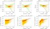 |
Fig. 4 Top panels: energy-period dependences of IMFs obtained with EMD of SDO/AIA data taken from the NOAA 11131 active region, ROI 1 from 00:00 to 03:20 UT, 8 December 2010. The spectral power and periods of individual IMF are shown by yellow dots. Total number of considered observational samples is 2500, containing 500 data points each. The 99% and 1% confidence intervals are shown with the black solid (white noise) and dashed (coloured noises) lines. The energy averaged over each period is indicated by the red crosses. Blue lines represent the empirical dependence of the mean modal energy upon the period, obtained with the linear fitting. Green lines show the general confidence interval for the superposition of the white and coloured noises. Bottom panels: Fourier spectral power-period dependences of the same data sets as shown in the top panels. The spectral power and periods of individual Fourier harmonics are shown by yellow dots. The red crosses indicate the mean Fourier spectra. The blue lines are the best linear fit showing the power-law-like regions of the spectra. Values of the power law index α with corresponding 1σ uncertainties are shown above each panel. |
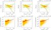 |
Fig. 5 The same as shown in Fig. 4 for the SDO/AIA data sets taken from the NOAA 11131 active region, ROI 2. |
We calculated the confidence intervals of 99% and 1% significances (see Fig. 4) for both random components in assumption of the chi-squared modal energy distribution given by Eq. (5). The maximal and minimal values of these intervals for each period give us a general confidence interval for the superposition of both processes. The general confidence intervals are indicated by the green solid lines in Figs. 4 and 5. Energies of IMFs of 171 Å and 304 Å signals in the top plots of Fig. 4 are located mainly inside the confidence intervals. The only exception is the first (the shortest period) IMFs which have the energies above the upper confidence limit. We note that the same feature of the first IMFs also appears in the energy-period distributions obtained for synthetic noises (see Fig. 2). Similar unusual behaviour of the first mode energy of the white noise samples was also reported in Wu & Huang (2004). Hence, we attribute this effect to the intrinsic artefact of the EMD technique and do not discuss it in further analysis.
The other SDO/AIA data set taken from a lower level of ROI 1, namely the intensity signals at 1600 Å, shows similar spectral energy distribution well localised inside the general confidence interval with α ≈ 0 and α ≈ 0.86. The latter proves that the intensity variations observed in the quiet sun regions can be definitely considered as a random process with the power law spectral density distribution. However, the second group of 1600 Å IMFs with periods being between three and four minutes is located partly outside the interval and hence cannot be attributed to the noise. As the 1600 Å observational wavelength corresponds to the electromagnetic emission coming from the upper photosphere, these IMFs are likely to be associated with some specific periodic processes operating at lower levels of the solar atmosphere.
Figure 5 shows the energy-period dependences of IMFs of 171 Å, 304 Å, and 1600 Å data sets taken from ROI 2. Similarly to the previous cases, the longer-period spectral components (with periods longer than aproximately ten minutes) can be described by the power law distribution with the index α being of about 1.26, 1.23, and 1.33, respectively. The spectral components with approximate periods shorter than two minutes are seen to be more related to the white noise distribution. As ROI 2 is located above the sunspot umbrae (see Fig. 3), EMD expansion of 171 Å and 304 Å data clearly gives a distinct group of IMFs with energies outside the general confidence interval. Their periods range approximately from two to four minutes, coinciding with typical periods of 3-min sunspot oscillations. Nearly the same periodicities can be also detected in the 1600 Å energy-period distribution. These results are in accord with the behaviour of the mean Fourier spectra which are also shown in Fig. 5.
4. Discussion and conclusions
We revealed empirical properties of synthetic coloured noises expanded via EMD, allowing for arbitrary values of the power law index α in the power spectral density S as a function of frequency, f written in the form S = 1 /fα. In analogy with Wu & Huang (2004) where the corresponding properties of the white noise (α = 0) are given, our findings can be briefly itemised as follows:
-
Based on the dyadic nature of EMD we found that the energydensity Em of IMFs obtained from the coloured noise samples with EMD is connected with the mean modal period Pm through the relation
 , derived in Eq. (7).
 -
Energies of IMFs of coloured noises were found to be chi-squared distributed, according to Eq. (5). The latter expression in turn reduces to the corresponding white noise distribution shown in Wu & Huang (2004), for the limiting case when α = 0 and the IMF’s numbers of DoF are proportional to the modal energies.
-
Numerical experiments performed with the use of synthetic coloured noise samples showed that the chi-squared distribution for Em is well applicable to the noises with values of the power law index α being of up to 2 (see Fig. 2). While for higher values of α, for example for α = 2 and α = 2.5 shown in Fig. 2, the distribution of modal energies is seen to have a rather different form. The latter fact is related to the dyadic properties of EMD, indicating that they are mainly pronounced for coloured noises with approximate α< 2, and are corrupted for noises with
 when correlation between data points is
sufficiently strong in a signal.
when correlation between data points is
sufficiently strong in a signal.
For illustration, we applied this EMD-based method for probing different layers of the solar atmosphere looking for the appearance of randomly distributed processes. We analysed intensity variation signals coming from two regions of interest: one is located above a quiet sun area, and another is above a sunspot, both are related to the NOAA 11131 active region. In particular, the analysed sunspot showed clear 3-min oscillations of a non-regular deep-modulated wave-train profile shape (see, e.g., Fig. 4 in Reznikova et al. 2012). Due to its adaptive nature, EMD was chosen as the most suitable method for processing such sort of signals. We found that the intensity variations of both quiet sun and sunspot regions at 171 Å (coronal level) and 304 Å (chromospheric level) indeed behave randomly and can be represented as a superposition of two noise-like processes with the corresponding power law index α ≈ 0 (the white noise component) at periods shorter than 2 minutes, and α ≈ 1.2−1.3 (the reddish noise) at longer periods. These findings are in consistence, e.g., with the results obtained recently in Ireland et al. (2015) with the use of the mean Fourier spectra for the coronal emission at 171 Å and 193 Å wavelengths. There, the power law indices were found to range from 1.8 to 2.3 for both wavelengths, depending upon the analysed region. In addition to the coronal (171 Å) and chromospheric (304 Å) lines, in this paper we also analysed the emission intensity variations at 1600 Å, corresponding to deeper layers of the solar atmosphere. Similarly to the upper levels, signals coming from 1600 Å emission layer are also seen to be well represented by a combination of the white and coloured noises. However, the corresponding coloured component experiences dramatic change in the power law index from about 0.86 to 1.33 when transiting from the quiet sun to the sunspot atmosphere. The latter means the domination of a low-frequency processes deep inside the sunspot atmosphere, while characteristic frequencies for the quiet sun area decrease with height. In contrast with the earlier works where the variations of slopes of the high-frequency spectral tails (at periods shorter than about 3 min) were considered (see, e.g. Deubner & Fleck 1990, Fig. 5; Woods & Cram 1981, Fig. 1; Orrall 1966, Fig. 4; and Evans et al. 1963, Fig. 3), we studied the evolution of the spectral slopes from the photosphere up to the corona in the extended range of periods up to 100 min. In addition to the randomly distributed background processes, groups of IMF with energies which are located significantly above the noise level, were also clearly detected by the method. In particular, their periods range from two to four minutes (for the sunspot regions) and may be clearly associated with 3-min sunspot oscillations. For the quiet sun region observed at 1600 Å, the energy distribution peaks at about four to five minutes, which can be considered as a manifestation of the p-modes.
We also calculated the mean Fourier spectra for the same data sets which were used in the EMD analysis. Results obtained with the Fourier technique are completely in accord with those obtained with EMD. In particular, the mean Fourier spectra were also found to contain the power-law-like regions at longer periods and tend to a flat shape at shorter periods, meaning that they also could be represented as a combination of the corresponding coloured and white noise-like components. We recall that by definition the EMD and Fourier techniques are essentially different and independent spectral approaches based upon different principles and intrinsic properties. Hence, a full agreement between the results obtained separately with these two methods in the paper evidently confirms the ability of EMD to detect random processes in solar signals, and justifies its applicability.
Acknowledgments
This work is supported by the European Research Council under the SeismoSun Research Project No. 321141 (SAA, VMN), the STFC consolidated grant ST/L000733/1, and the BK21 plus program through the National Research Foundation funded by the Ministry of Education of Korea (VMN).
References
- Bárta, M., Büchner, J., Karlický, M., & Skála, J. 2011, ApJ, 737, 24 [NASA ADS] [CrossRef] [Google Scholar]
- Bazilevskaya, G., Broomhall, A.-M., Elsworth, Y., & Nakariakov, V. M. 2014, Space Sci. Rev., 186, 359 [NASA ADS] [CrossRef] [Google Scholar]
- Christensen-Dalsgaard, J. 2002, Rev. Mod. Phys., 74, 1073 [NASA ADS] [CrossRef] [Google Scholar]
- De Moortel, I., & Nakariakov, V. M. 2012, Phil. Trans. R. Soc. London Ser. A, 370, 3193 [Google Scholar]
- Deng, L. H., Li, B., Xiang, Y. Y., & Dun, G. T. 2015, J. Atm. Sol. Terrestr. Phys., 122, 18 [Google Scholar]
- Deres, A. S., & Anfinogentov, S. A. 2015, Astron. Rep., 59, 959 [NASA ADS] [CrossRef] [Google Scholar]
- Deubner, F.-L., & Fleck, B. 1990, A&A, 228, 506 [NASA ADS] [Google Scholar]
- Evans, J. W., Michard, R., & Servajean, R. 1963, Annales d’Astrophysique, 26, 368 [NASA ADS] [Google Scholar]
- Flandrin, P., Rilling, G., & Goncalves, P. 2004, IEEE Signal Proc. Lett., 11, 112 [NASA ADS] [CrossRef] [EDP Sciences] [Google Scholar]
- Franzke, C. 2009, Nonl. Proc. Geophys., 16, 65 [NASA ADS] [CrossRef] [Google Scholar]
- Gao, P.-X., Xie, J.-L., & Liang, H.-F. 2012, Res. Astron. Astrophys., 12, 322 [NASA ADS] [CrossRef] [Google Scholar]
- Gruber, D., Lachowicz, P., Bissaldi, E., et al. 2011, A&A, 533, A61 [NASA ADS] [CrossRef] [EDP Sciences] [Google Scholar]
- Hathaway, D. H. 2010, Liv. Rev. Sol. Phys., 7, 1 [Google Scholar]
- Huang, N. E., & Wu, Z. 2008, Rev. Geophys., 46, RG2006 [NASA ADS] [CrossRef] [Google Scholar]
- Huang, N. E., Shen, Z., Long, S. R., et al. 1998, Roy. Soc. Lond. Proc. Ser. A, 454, 903 [NASA ADS] [CrossRef] [Google Scholar]
- Inglis, A. R., Ireland, J., & Dominique, M. 2015, ApJ, 798, 108 [NASA ADS] [CrossRef] [Google Scholar]
- Ireland, J., Marsh, M. S., Kucera, T. A., & Young, C. A. 2010, Sol. Phys., 264, 403 [NASA ADS] [CrossRef] [Google Scholar]
- Ireland, J., McAteer, R. T. J., & Inglis, A. R. 2015, ApJ, 798, 1 [NASA ADS] [CrossRef] [Google Scholar]
- Jess, D. B., Morton, R. J., Verth, G., et al. 2015, Space Sci. Rev., 190, 103 [NASA ADS] [CrossRef] [Google Scholar]
- Kolotkov, D. Y., Broomhall, A.-M., & Nakariakov, V. M. 2015a, MNRAS, 451, 4360 [NASA ADS] [CrossRef] [Google Scholar]
- Kolotkov, D. Y., Nakariakov, V. M., Kupriyanova, E. G., Ratcliffe, H., & Shibasaki, K. 2015b, A&A, 574, A53 [NASA ADS] [CrossRef] [EDP Sciences] [Google Scholar]
- Kupriyanova, E. G., Melnikov, V. F., Nakariakov, V. M., & Shibasaki, K. 2010, Sol. Phys., 267, 329 [NASA ADS] [CrossRef] [Google Scholar]
- Lee, J. N., Cahalan, R. F., & Wu, D. L. 2015, J. Atm. Sol. Terrestr. Phys., 132, 64 [Google Scholar]
- Liu, W., & Ofman, L. 2014, Sol. Phys., 289, 3233 [NASA ADS] [CrossRef] [Google Scholar]
- Martens, P. C. H., Attrill, G. D. R., Davey, A. R., et al. 2012, Sol. Phys., 275, 79 [NASA ADS] [CrossRef] [Google Scholar]
- McAteer, R. T. J., Young, C. A., Ireland, J., & Gallagher, P. T. 2007, ApJ, 662, 691 [NASA ADS] [CrossRef] [Google Scholar]
- Nagovitsyn, Y. A. 1997, Astron. Lett., 23, 742 [NASA ADS] [Google Scholar]
- Nakariakov, V. M., & King, D. B. 2007, Sol. Phys., 241, 397 [NASA ADS] [CrossRef] [Google Scholar]
- Nakariakov, V. M., & Melnikov, V. F. 2009, Space Sci. Rev., 149, 119 [NASA ADS] [CrossRef] [Google Scholar]
- Nakariakov, V. M., Inglis, A. R., Zimovets, I. V., et al. 2010, Plasma Physics and Controlled Fusion, 52, 124009 [Google Scholar]
- Orrall, F. Q. 1966, ApJ, 143, 917 [NASA ADS] [CrossRef] [Google Scholar]
- Qu, Z.-N., Feng, W., & Liang, H.-F. 2015, Res. Astron. Astrophys., 15, 879 [NASA ADS] [CrossRef] [Google Scholar]
- Reznikova, V. E., Shibasaki, K., Sych, R. A., & Nakariakov, V. M. 2012, ApJ, 746, 119 [NASA ADS] [CrossRef] [Google Scholar]
- Simões, P. J. A., Hudson, H. S., & Fletcher, L. 2015, Sol. Phys., 290, 3625 [NASA ADS] [CrossRef] [Google Scholar]
- Sych, R., & Nakariakov, V. M. 2014, A&A, 569, A72 [NASA ADS] [CrossRef] [EDP Sciences] [Google Scholar]
- Sych, R. A., Nakariakov, V. M., Anfinogentov, S. A., & Ofman, L. 2010, Sol. Phys., 266, 349 [NASA ADS] [CrossRef] [Google Scholar]
- Terradas, J., Oliver, R., & Ballester, J. L. 2004, ApJ, 614, 435 [NASA ADS] [CrossRef] [Google Scholar]
- Vecchio, A., Laurenza, M., Meduri, D., Carbone, V., & Storini, M. 2012, ApJ, 749, 27 [NASA ADS] [CrossRef] [Google Scholar]
- Woods, D. T., & Cram, L. E. 1981, Sol. Phys., 69, 233 [NASA ADS] [CrossRef] [EDP Sciences] [Google Scholar]
- Wu, Z., & Huang, N. E. 2004, Proc. R. Soc. Lond. Ser. A, 460, 1597 [Google Scholar]
- Wu, Z., & Huang, N. E. 2009, Adv. Adaptive Data Analysis, 1, 1 [Google Scholar]
- Yuan, D., Sych, R., Reznikova, V. E., & Nakariakov, V. M. 2014, A&A, 561, A19 [NASA ADS] [CrossRef] [EDP Sciences] [Google Scholar]
- Zolotova, N. V., & Ponyavin, D. I. 2007, Sol. Phys., 243, 193 [Google Scholar]
All Figures
|
Fig. 1 Histograms (black) showing the normalised modal energy NEm fitted by distribution (5) (red) for several IMFs obtained with EMD from 2000 independent samples of the synthetic white (α = 0, left column) and coloured (α = 1.5, right column) noises. Each noise sample contains N = 500 data points. All samples were normalised for their total energy to be unity. |
| In the text | |
|
Fig. 2 Energy-period distributions (yellow dots) of IMFs obtained with EMD from 2000 independent samples of synthetic noisy signals with α = 0 (the white noise), α = 0.5, α = 1 (flicker or the pink noise), α = 1.5, α = 2 (Brown(ian) or the red noise), and α = 2.5. Each sample contains 500 data points. All samples were normalised for their total energy to be unity. Period is measured in dimensionless evenly sampled time-steps between the data points. The energy averaged over each period is indicated by the red crosses. Blue lines represent the empirical dependence of the mean modal energy |
| In the text | |
|
Fig. 3 Active region NOAA 11131 observed with SDO/AIA at the 171 Å (top), 304 Å (middle), and 1600 Å (bottom) wavelengths. Images are taken at 00:00:00 UT, 8 December 2010. White squares show the regions of interest (ROI) for intensity variations considered in this paper. |
| In the text | |
|
Fig. 4 Top panels: energy-period dependences of IMFs obtained with EMD of SDO/AIA data taken from the NOAA 11131 active region, ROI 1 from 00:00 to 03:20 UT, 8 December 2010. The spectral power and periods of individual IMF are shown by yellow dots. Total number of considered observational samples is 2500, containing 500 data points each. The 99% and 1% confidence intervals are shown with the black solid (white noise) and dashed (coloured noises) lines. The energy averaged over each period is indicated by the red crosses. Blue lines represent the empirical dependence of the mean modal energy upon the period, obtained with the linear fitting. Green lines show the general confidence interval for the superposition of the white and coloured noises. Bottom panels: Fourier spectral power-period dependences of the same data sets as shown in the top panels. The spectral power and periods of individual Fourier harmonics are shown by yellow dots. The red crosses indicate the mean Fourier spectra. The blue lines are the best linear fit showing the power-law-like regions of the spectra. Values of the power law index α with corresponding 1σ uncertainties are shown above each panel. |
| In the text | |
|
Fig. 5 The same as shown in Fig. 4 for the SDO/AIA data sets taken from the NOAA 11131 active region, ROI 2. |
| In the text | |
Current usage metrics show cumulative count of Article Views (full-text article views including HTML views, PDF and ePub downloads, according to the available data) and Abstracts Views on Vision4Press platform.
Data correspond to usage on the plateform after 2015. The current usage metrics is available 48-96 hours after online publication and is updated daily on week days.
Initial download of the metrics may take a while.