| Issue |
A&A
Volume 592, August 2016
|
|
|---|---|---|
| Article Number | A98 | |
| Number of page(s) | 9 | |
| Section | Extragalactic astronomy | |
| DOI | https://doi.org/10.1051/0004-6361/201528030 | |
| Published online | 04 August 2016 | |
Highly ionized disc and transient outflows in the Seyfert galaxy IRAS 18325–5926
1 Institut de Ciències del Cosmos (ICCUB), Universitat de Barcelona (IEEC-UB), Martí i Franquès, 1, 08028 Barcelona, Spain
e-mail: This email address is being protected from spambots. You need JavaScript enabled to view it.
2 ICREA, Pg. Lluís Companys 23, 08010 Barcelona, Spain
3 Institute of Astronomy, Madingley Road, Cambridge CB3 0HA, UK
4 Department of Astronomy, University of Maryland, College Park, MD 20742-2421, USA
5 Centro de Astrobiologia (CSIC-INTA), Dep. de Astrofísica, ESAC, PO Box 78, 28691 Villanueva de la Cañada, Madrid, Spain
6 X-ray Astrophysics Laboratory and CRESST, NASA/Goddard Space Flight Center, Greenbelt, MD 20771, USA
Received: 22 December 2015
Accepted: 10 June 2016
Abstract
We report on strong X-ray variability and the Fe K-band spectrum of the Seyfert galaxy IRAS 18325–5926 obtained from the 2001 XMM-Newton EPIC pn observation with a duration of ~120 ks. While the X-ray source is highly variable, the 8–10 keV band shows larger variability than that of the lower energies. Amplified 8–10 keV flux variations are associated with two prominent flares of the X-ray source during the observation. The Fe K emission is peaked at 6.6 keV with moderate broadening. It is likely to originate from a highly ionized disc with an ionization parameter of log ξ ≃ 3. The Fe K line flux responds to the main flare, which supports its disc origin. A short burst of the Fe line flux has no relation to the continuum brightness, for which we have no clear explanation. We also find transient, blueshifted Fe K absorption features that can be identified with high-velocity (~0.2c) outflows of highly ionized gas, as found in other active galaxies. The deepest absorption feature appears only briefly (~1 h) at the onset of the main flare and disappears when the flare declines. The rapid evolution of the absorption spectrum makes this source peculiar among the active galaxies with high-velocity outflows. Another detection of the absorption feature also precedes the other flare. The variability of the absorption feature partly accounts for the excess variability in the 8–10 keV band where the absorption feature appears. Although no reverberation measurement is available, the black hole mass of ~2 × 10⁶M⊙ is inferred from the X-ray variability. When this mass is assumed, the black hole is accreting at around the Eddington limit, which may fit the highly ionized disc and strong outflows observed in this galaxy.
Key words: galaxies: active / galaxies: Seyfert / X-rays: galaxies
© ESO, 2016
1. Introduction
IRAS 18325–5926 (=Fairall 49) is one of the early X-ray selected active galactic nuclei (AGN) of Piccinotti et al. (1982), identified with an obscured Seyfert nucleus hosted by the IRAS galaxy at z = 0.0198 (Ward et al. 1988; Carter 1984; de Grijp et al. 1985; Strauss et al. 1992; Iwasawa et al. 1995). The nuclear X-ray source is moderately absorbed by NH ≈ 1 × 1022 cm-2 and shows strong flux variability. The X-ray spectrum shows a strong iron emission feature (Fe K). The line profile appears broad and peaks at 6.6 keV, which Iwasawa et al. (1996, 2004b) suggested to originate from reflection of an highly ionized disc (but see Lobban & Vaughan 2013). This is unusual among nearby bright AGN in which a cold line at 6.4 keV is the normal Fe K feature, suggesting that this active nucleus may be operating in an extreme condition.
XMM-Newton observations of IRAS 18325–5926 have been made in 2001 and 2013 with exposure times of 120 ks and 200 ks, respectively. In the recent 2013 observation, in which two 100 ks exposures are separated by three weeks, Lobban et al. (2014) found hard X-ray lags. For the 2001 observation, data from the two EPIC MOS cameras, MOS1 and MOS2, have been extensively analysed for the composition of the broad-band X-ray spectrum and its variability by Tripathi et al. (2013) and Lobban & Vaughan (2013), while only the time-averaged spectrum was briefly presented for the EPIC pn data in Iwasawa et al. (2004b). Here we focus on the Fe-K band spectrum and its variability during the 2001 observation, using the EPIC pn data, since the pn camera has a higher sensitivity for the Fe K band and it is clearly advantageous to study this photon-limited band over the MOS cameras.
The cosmology adopted here is H0 = 70 km s-1 Mpc-1, ΩΛ = 0.72, ΩM = 0.28.
2. Observations
We observed IRAS 18325–5926 with XMM-Newton in a full orbit of revolution 227 on 2001 March 5–7 (ObsID 0022940301, PI: K. Iwasawa). The EPIC pn camera was operating in small window mode with the medium filter. As no disruptive background flares occurred during the observation, we used the whole duration of the observation of approximately 118 ks. With the efficiency of the small window mode (~70%), the net exposure time is 81.5 ks.
The mean (net) count rate from the X-ray source in the 2–10 keV band is 1.330 ± 0.004 ct s-1. The background count rate has a small fraction (≃1%) of the source count rate in the same band.
3. Results
3.1. Mean broad-band spectrum
The broad-band (2–11 keV) X-ray spectrum obtained with the EPIC pn camera is shown in Fig. 1. The spectrum is plotted in 200 eV intervals. It shows a low energy cut-off due to the moderate absorption of NH ~ 1022 cm-2, which is probably caused by cold gas in the host galaxy, for example, dust lanes imaged by HST (Malkan et al. 1998), as discussed in Iwasawa et al. (1995). The warm absorber detected in the Chandra HETGS has the ionization parameter ξ = L/ (nR2), where L is the ionizing luminosity, n is the density of the ionized matter, and R is the distance from the ionizing source, of log ξ = 2.0 (erg cm s-1), with a column density of NH = 1.5 × 1021 cm-2 (Mocz et al. 2011), which modifies the spectrum below ~2.3 keV but has little effect at higher energies. To avoid unnecessary complication by this warm absorber and a possible contamination from an extranuclear emission appearing at lower energies, we limit our spectral study of the nuclear emission to above 2.3 keV (where a discontinuity of the telescope response due to Au edges is present). Fitting a simple power-law to the 2.3–11 keV continuum gives a photon index Γ = 2.08 ± 0.02 and a cold absorption column density of NH = (1.3 ± 0.1) × 1022 cm-2, as measured in the galaxy rest-frame (Table 1). A power-law was used to describe the continuum spectrum for the analysis below unless stated otherwise, and this cold absorption was assumed to be constant. The Fe K emission at 6–7 keV is clearly detected, and there are possible absorption features on the blue side, as indicated by arrows in Fig. 1.
 |
Fig. 1 Upper panel: the 2–11 keV spectrum of IRAS 18325–5926 obtained from the EPIC pn camera. The vertical axis is in flux units (EFE) and the horizontal axis is the energy (keV) as observed. The spectrum is plotted in 200 eV intervals. Two possible blueshifted Fe K absorption features are marked by red arrows. Lower panel: details of the Fe-K band spectrum with 90-eV energy intervals. The dotted and solid line histograms show the best-fit models with xillver (log ξR ~ 3.5) and reflionx (log ξR ~ 3.2), respectively. No relativistic blurring is included. The resolved narrow line cores of Fe xxv and Fe xxvi of xillver do not agree with the smooth, broad profile of the data, whereas the reflionx model fits well (see text). A narrow line feature is seen at the observed energy at the rest-frame 6.4 keV, as indicated by the vertical dotted line. |
The Fe-K band spectrum is shown in Fig. 1b. The line profile is broad and largely smooth at the EPIC pn resolution ~150 eV in FWHM in the Fe K band at the epoch of observation (XMM-Newton Users Handbook 2.13.1). When a Gaussian is fitted, the Fe K emission is found to have a centroid energy of 6.61 ± 0.04 keV, a dispersion of σ = 0.45 ± 0.05 keV (or FWHM ≈ 48 000 km s-1), and an intensity of (3.8 ± 0.4) × 10-5 phcm-2s-1, as measured in the rest-frame. This result is robust against continuum modelling (see Table 1) and agrees with that from the MOS cameras (see Tripathi et al. 2013). The corresponding equivalent width (EW) is 0.28 ± 0.03 keV. The line centroid energy is significantly higher than 6.4 keV, which probably indicates that the emission line originates in reflection from a highly ionized medium (see Iwasawa et al. 1996, for a discussion of the hypothesis of cold reflection from an inclined disc), but its origin is discussed in detail in Sect. 3.4. In the case of reflection from an ionized disc, the main ionization stage of iron ions would be Fe xxv with ξ of the order of 103 erg cm s-1. In addition to the broad emission, a small spike is found at the rest-frame 6.4 keV. Constraints on the energy and width of this narrow feature need the data of 90 eV binning, as shown in Fig. 1b, compatible with the spectral resolution. Fitting a narrow Gaussian to this feature gives a 3σ detection with an intensity of I = (3.1 ± 1.0) × 10-6 phcm-2s-1 and a corresponding EW of ≃20 eV, indicating that the contribution of reflected light from distant cold matter is minor.
Mean EPIC pn spectrum of IRAS 18325–5926.
Two possible absorption features are found at 8.43 ± 0.11 keV and 9.65 ± 0.12 keV (as measured in the galaxy rest-frame). They may be blueshifted high-ionization Fe K absorption lines originating from high-velocity outflows, as found in a number of Seyfert galaxies and quasars (e.g. Reeves et al. 2009; Pounds et al. 2006; Chartas et al. 2002, 2003; Tombesi et al. 2010; Vignali et al. 2015), but their detection is not secure here on statistical grounds. These absorption features are found to be transient and appear strongly in limited time intervals, as shown below, where a statistical test supports their detection. They are therefore diluted in the mean spectrum, leaving only a weaker trace of their presence. We examine the absorption features in the mean spectrum first. The same method is applied for transient absorption features presented in the later section.
The statistical test for the absorption-line feature was adopted from Tombesi et al. (2010, see also Zoghbi et al. 2015). An absorbed power-law plus a Gaussian (for the Fe K emission) was used as a base-line model. The reduction of χ2 when a Gaussian absorption line is introduced to explain the spectral drops at 8.4 keV and 9.6 keV is comparable with Δχ2 = −4.4 for both features. With this χ2 reduction set to the target Δχ2, improvements of fit quality were examined for 1000 faked spectra simulating the base-line model when a narrow Gaussian was introduced in the 7–10 keV range (because a highly blueshifted Fe K absorption line can appear anywhere in this energy range, depending on the outflowing velocity of the absorbing matter). The probability to have a false line feature exceeding the target Δχ2 was found to be P = 0.3. Thus each of the possible absorption features has no statistical significance. However, the chance probability of two absorption features with Δχ2 = −4.4 at the same time, as seen in Fig. 1, is deduced to be P ≃ 0.3 × 0.3 = 0.09. Detection of transient absorption features at higher significance are presented in Sect. 3.3. Given the transient nature and variability of the absorption as described below, the results of the spectral fitting with the XSTAR model for absorption by photoionized gas presented in Table 1 may not reflect the true properties of the absorber. Details of the XSTAR model are described in Sect. 3.3.1.
3.2. Flux variability
The mean 2–10 keV flux during the XMM-Newton observation was 1.4 × 10⁻¹¹ ergs-1cm-2, at the lowest level compared to the other observations of this source (Iwasawa et al. 2004b). The corresponding 2–10 keV luminosity corrected for the internal absorption (obtained from the absorbed power-law fit to the continuum) is 1.5 × 1043 ergs-1.
 |
Fig. 2 Light curve of IRAS 18325-5926 during the XMM-Newton observation obtained from the EPIC pn. The count rates in the 1–8 keV band corrected for background in 256-s intervals are plotted. |
3.2.1. Variability amplitude as a function of energy
The 1–8 keV light curve is shown in Fig. 2. The fractional rms variability amplitude, Fvar (Vaughan et al. 2003), is 0.22 ± 0.02. The variability is dominated by a strong flare around 70 ks, where the X-ray flux rises from the lowest flux to the highest of the observation by a factor of 3 within 15 ks. A weaker broad flare is also seen around 30 ks. Figure 3 shows Fvar as a function of energy. The light curves of 2 ks bins in the five bands corrected for background were used to compute these Fvar.
 |
Fig. 3 Fractional rms variability amplitude (Fvar, Vaughan et al. 2003) as a function of energy is plotted in the 1–10 keV band. They were obtained from background-corrected light curves in the respective bands for the whole 118 ks duration with 2-ks time bins. |
Fvar in the 1–2 keV band drops below the level of the 2–8 keV band. This decline continues towards lower energies and can be understood if a contribution of the constant (or weakly variable) emission from an extranuclear region, which has been discussed in Iwasawa et al. (1996) and Tripathi et al. (2013), becomes significant below 2 keV. This justifies the use of the energy range above 2.3 keV for our spectral analysis of the central source.
 |
Fig. 4 Light curves of the whole observation in 2–5 keV (blue), 5–8 keV (red), and 8–10 keV (green) bands, normalised to the mean count rate in the respective bands. The resolution of the light curve is 1 ks for the two lower energy bands and 2 ks for the 8–10 keV bands. The three intervals during the main flare, (i), (ii), and (iii), are indicated (see Sect. 3.3.1, Fig. 6). |
Notable is the excess of Fvar in the 8–10 keV band above that of the lower energies. This cannot be an artefact caused by incorrect background correction. The background is, on average, only at a level of 5 per cent of the 8–10 keV counts. The background light curves taken from the source-free region is not correlated with the source light curve, and at the interval of the strongest variation, that is, the flare around 70 ks, the background is most quiet. A similar excess of Fvar in the 8–10 keV band is also seen in the 2013 observation (Lobban et al. 2014).
3.2.2. Shape of the light curve as a function of energy
The shape of the light curve varies as a function of energy. The background-corrected light curves in the 2–5 keV, 5–8 keV, and 8–10 keV, normalised by the respective mean count rates, are plotted in Fig. 4. The normalised light curve apparently shifts behind in time with increasing energies. This is most notable around the two broad flares at ~30 ks and ~70 ks. The 8–10 keV band, in particular, shows a clear displacement there from the other lower energy bands. The timing analysis for the 2013 observation by Lobban et al. (2014) found a hard lag up to 4 ks, which is qualitatively consistent with the above finding.
Except for the small hard lag, the 2–5 keV and 5–8 keV bands are quite similar in shape and amplitude. Little or no offset in normalisation is seen between the two curves. It corresponds that there is little or no offset in the flux correlation diagram for the two bands. This means that any constant component with a spectral shape distinctively different from the variable power-law, such as cold reflection originating from large radii, as often seen in nearby Seyfert galaxies, has a minor contribution. If any constant component were present, it would have a similar spectral shape as the primary power-law, for example, reflection from high-ionization medium.
The amplitude of the 8–10 keV normalised light curve is larger than the other two, as also evident in Fig. 3, which causes it to weave through those of the lower energy bands. The crossing points, where the 8–10 keV curve rises above those of the lower energies from beneath, coincide with the peaks of the two broad flares. While the lagged production of hard X-rays may be accompanied by an amplification of their flux, the variability of the blueshifted Fe absorption might, at least partly, account for the excess variability in the 8–10 keV band, since the absorption uniquely occurs in the band. This hypothesis with variable absorption and implications from the behaviour of the 8–10 keV normalised light curve are investigated below.
3.3. Fe-K band variability
With the X-ray brightness of this source, spectral variability on short timescales can be studied. To obtain a trend for the variability of the Fe K spectral features of interest over the whole observation, we generated an excess emission map, similar to that used in Iwasawa et al. (2004b). It is a map of excess emission (corrected for the detector response) on the time-energy plane above the continuum estimated for each time bin. The Fe K emission and absorption features are relatively broad, and to ensure that each spectral bin has sufficient counts, we chose a spectral resolution of 0.5 keV and set the time resolution to 2 ks. Each spectrum has at least 1000 counts in the 2.3–10 keV band even in the faintest interval. The continuum spectrum was modelled by fitting an absorbed power-law to the 3.3–10 keV data, excluding the spectral bin of the Fe emission line peak. The excess map with light smoothing is shown in Fig. 5. We also show the projected light curves in the three bands, which correspond to the Fe K line core (5.8–7.3 keV), the red wing (4.3–5.8 keV), and the blueshifted absorption (8–10 keV), that we extracted from the map. The adjusted continuum light curve is overplotted in red for reference along the Fe line core light curve.
In general, the data for the Fe-K band features do not show a tight correlation with the continuum flux. However, there are a few events that possibly warrant a further investigation. The line core curve shows a strong rise in flux in two time regions around 76 ks and 96 ks. The first rise over the 8 ks interval roughly coincides with the main flare, suggesting that the line emission responds to the continuum. Incidentally, just before the Fe K line flux rise, the blue absorption band shows a sharp fall of the flux around 70 ks. Since these notable variations in the Fe K band are associated with the main flare where the most dramatic flux change in the observation occurs, we investigate the spectral evolution during this interval first (Sect. 3.3.1).
3.3.1. Rapid evolution of the absorption spectrum during the main flare
Based on the χ2 reduction by introducing a Gaussian, the 2 ks interval spectra around the main flare were examined for a blueshifted Fe K absorption feature. The two intervals of strongest suppression in the blue absorption band in the excess map in the 68–72 ks range are verified to have the deepest absorption features with an equal amount of χ2 reduction (Δχ2 = −11) when a Gaussian absorption line is introduced. These two intervals are found at similar energies, 8.9 ± 0.2 keV and 8.6 ± 0.2 keV, as measured in the rest frame.
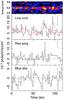 |
Fig. 5 From top to bottom: the excess map in the time-energy plane with a resolution of 2 ks in time and 0.5 keV in energy. Light smoothing with an elliptical Gaussian kernel (2 pixel × 1 pixel in FWHM) was applied. The three light curves are derived from the excess map by projecting the multiple spectral channels, corresponding to the Fe K line core centred on the 6.5 keV (5.75–7.25 keV) and the red wing (4.25–5.75 keV), and the blueshifted absorption band (7.75–9.75 keV). The histograms were obtained from the unsmoothed map, while the grey lines stem from the smoothed map. The typical measurement error in each band is shown. In the panel of the Fe K line core variability, the 2–5 keV continuum light curve (the red solid line: adjusted to the mean and variance of the line variation) is overplotted for reference. |
This interval is also where the normalised 8–10 keV light curve lies well below those of the lower energy bands (Fig. 4). Using the simulation method, the chance probability of the χ2 reduction in each 2 ks spectrum was found to be P = 0.015. Since this occurs over two continuous time-bins in the whole observation of total 59 bins (which represent the number of trials), the chance probability is deduced to be P = 0.015 × 0.015 × 59 ≃ 0.013. This value is valid for an absorption line in each spectrum appearing anywhere in the 7–10 keV. Since the two intervals show absorptions at energies consistent with each other, the true chance probability is probably lower than 0.013. The spectrum combining the two intervals (denoted (i) in Fig. 5: 68–74 ks) is shown in Fig. 6. A deep absorption feature at ≃8.7 keV is evident. The χ2 reduction when a Gaussian absorption line is introduced is a Δχ2 = −21, which none of 1000 simulations with the baseline model reaches.
Variability of the blueshifted absorber
The absorption spectrum was modelled by the photoionized absorber computed by XSTAR (Kallman & Bautista 2001). A relatively broad width (σ = 0.4 ± 0.2 keV) and a large line EW of ~−0.6 keV suggest contributions of both Fe xxv and Fe xxvi with a high turbulent velocity (>1000 km s-1) of the absorber (see the curve-of-growth analysis presented in Tombesi et al. 2011). Thus we used an XSTAR table for absorption in photoionized gas with vturb = 5000 km s-1 (Vignali et al. 2015; Tombesi et al. 2011). Fitting the XSTAR table gives an ionization parameter of the absorber of log ξO = 3.3 ± 0.2, a column density of  cm-2, and an outflow velocity v = 0.23 ± 0.02c (Table 2). The Fe emission line in this spectrum is weak without clear broadening (σ< 0.4 keV, see Table 3). For this short interval, softer X-rays rise earlier, resulting in a softer continuum spectrum Γ = 2.5 ± 0.2.
The interval investigated above corresponds to the rising part of the main flare. The following two intervals of 8 ks each correspond to the flare peak (ii) 72–80 ks and the declining part (iii) 80–88 ks (Fig. 4), and their spectra are shown in Fig. 6. Interval (ii) coincides with the time range of the high Fe line core flux (Fig. 5). The Fe line flux measured by fitting a Guassian for the three intervals is shown in Table 3. The strong absorption observed in (i) may reduce the disc illumination, which results in the weak line flux. During interval (ii), the line flux seems to respond to the continuum brightening. Scattering from the outflow observed in (i) could add some line flux and shape the broad profile as well. The Fe emission line in (ii) is strong and broad with a redwards extension, which moves the Gaussian centroid to a lower energy than usual (Table 3). The three normalised light curves match in interval (ii), indicating that the broad-band spectral shape agrees with that of the mean spectrum and that the absorption feature in the 8–10 keV band has returned to the average depth. The 8–10 keV band curve in Fig. 4 rises above those of the lower energies in (iii), where the blue absorption feature disappears (Fig. 6, the 90% upper limit on the column density is NH < 1.2 × 1022 cm-2, assuming the same ξO and blueshift for (i), Table 2).
 |
Fig. 6 Spectral evolution seen during the large flare. The 3–10 keV spectra taken from (i) 68–72 ks; (ii) 72–80 ks; and (iii) 80–88 ks in Fig. 4 are shown. The histogram indicates the best-fit photoionized absorption model (see text). The Fe K emission lines are modelled by a Gaussian. The dotted line indicates the observed energy of 6.5 keV where the mean Fe K line peaks. |
Variability of Fe K emission.
3.3.2. Repeated absorption spectrum evolution?
 |
Fig. 7 Left: the 2.3–11 keV spectra taken from the two intervals, A 0–30 ks and B 30–60 ks, in the light curve. The spectra are plotted in 200-eV intervals with the best-fit model of the blueshifted ionized absorption computed by XSTAR (see text). Right: the χ2 curve as a function of energy, when scanning with a narrow Gaussian for absorption lines in the 7–10 keV range for the corresponding spectra. |
The dramatic spectral evolution in the blue absorption band occurs within 30 ks around the main flare. These absorption variations can be traced by the behaviour of the 8–10 keV normalised light curve relative to that of 5–8 keV (Fig. 4). Guided by Fig. 4, we assumed that a similar spectral evolution might be taking place across the other flare in the first half (0–60 ks) of the observation, albeit in a less dramatic fashion over a longer time range. Two time intervals with contrasting 8–10 keV behaviours were investigated.
Figure 7 shows the spectra taken from the intervals of 0–30 ks (A) and 30–60 ks (B). As above, absorption features were searched by scanning the 7–10 keV by a narrow Gaussian, and the resulting χ2 reduction is plotted in the right panel for each spectrum. The largest reduction in χ2 is found at 8.3 keV in the interval A spectrum with Δχ2 = −13. The statistical test finds the chance probability for this feature to be P ≃ 0.018 (including the number of trials of 3). Furthermore, another absorption feature with Δχ2 = −5.5 is seen at 9.7 keV in the interval A spectrum. None of 1000 simulated spectra show two line features, regardless of energy, at the same time with χ2 reductions comparable or larger than those two observed absorption features, suggesting a chance probability of P< 0.003. Therefore we consider a detection of the absorption features in interval A as likely. Fitting the XSTAR table to the stronger 8.3 keV feature gives log  , NH = (3.8 ± 1.5) × 1022 cm-2, and v = 0.19 ± 0.01c (Table 2). The weaker 9.7 keV absorption feature coincides with the Kβ transitions, but the observed depth is larger than expected. If it originates instead from a higher velocity system, its blueshift would be v = 0.30 ± 0.01c, assuming the same ionization parameter for the 8.3 keV absorption. On the other hand, the spectrum of interval B shows no clear sign of the absorption feature seen in the interval A spectrum. Interval B is the post-flare interval, as the (iii) interval of Fig. 6, where the absorption feature disappears.
3.3.3. Sharp increase in the Fe K line flux
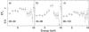 |
Fig. 8 Spectrum of the interval of a short burst of the Fe K line core flux (94–98 ks, see Fig. 5, Sect. 3.3.3) is shown in panel b). The spectra of the neighbouring intervals with the same 4 ks durations are shown in panels a) and c). |
The 94–98 ks interval shows a sharp rise in Fe K emission flux (Fig. 5) that is not accompanied by any obvious continuum flux increase. The two consecutive time bins of 2 ks intervals show exceptionally strong line flux in the core band, even stronger than those during the major flare (see Table 3). This band is where the Fe K emission is expected, therefore we examined how statistically reliable the high intensities seen in those intervals are, again using simulated spectra with Fe K emission of the mean spectrum. The line core flux was derived for each simulated spectrum following the same procedure to generate the excess map and the light curve in Fig. 5. The chance probabilities for the fluxes of 94–96 ks and 96–98 ks are <0.001 and 0.01, respectively. These two intervals of strong intensity occur in a row in the whole observations of 59 time intervals, which implies the chance probability to P< 6 × 10⁻⁴. A detection of the Fe line flux increase in this short interval is likely. Figure 5 suggests that it is also accompanied by a flux increase in the red wing.
Figure 8 shows the spectrum of the 94–98 ks interval along with the preceding and following intervals of 4 ks. The strong line core in the 94–98 ks spectrum is evident in contrast to the spectra of the neighbouring intervals, although broad emission down to 5 keV may be seen in both panels. The line flux of the 94–98 ks interval obtained by fitting a Gaussian is (9.2 ± 2.2) × 10-5 phcm-2s-1, is factor of ~3 larger than the mean value (Table 1). The continuum level comparable to the mean flux leads to an extremely large EW of 0.90 ± 0.21 keV. This large EW is a result of the increase in absolute line flux. A Fe K line this strong in absence of a continuum increase is difficult to understand unless the illuminating source temporarily becomes anisotropic. Gravitational light focusing effect (e.g. Martocchia & Matt 1996; Miniutti & Fabian 2004) is not compatible with the line shape because it does not match the expected extreme gravitational redshift. Anisotropy needs to be an intrinsic property of the illuminating source. We note that although not as extreme as this, unusually strong Fe K emission (EW ~ 0.6 keV) has occasionally been observed in previous ASCA observations (Iwasawa et al. 2004b), suggesting that similar bursts of Fe K line emission occur routinely in this source.
3.3.4. Broad emission component
The red wing band flux fluctuates around null in the first half of the observation but seems to show a systematic excess in the second half (Fig. 5). When a Gaussian is fitted to the Fe K line profile of the spectra taken from the two halves, the line widths are σ = 0.36 ± 0.05 keV in the first half and σ = 0.60 ± 0.09 keV in the second half, respectively, while the line centroid energies are compatible (6.62 ± 0.04 keV to 6.54 ± 0.07 keV, respectively). The enhanced line broadening can come either from increased ξR (due to Compton broadening) or stronger gravitational effects. Given that the mean source luminosity is comparable between the two intervals, increased relativistic effect is a more likely cause. This suggests that the line-emitting region has moved inwards in the latter half of the observation, which is examined further with the relativistic blurring model below.
3.4. Modelling the reflection spectrum
As shown above, the Fe-K band spectrum of IRAS 18325–5926 is variable. The blueshifted absorption features appear in limited time intervals, indicating that they are associated with transient outflows. The Fe K emission line is, in contrast, a persistent feature throughout the observation (Fig. 5) and maintains a similar shape apart from some intervals of dramatic variability examined in Sect. 3.3. This favours a hypothesis that the line originates primarily in reflection from the accretion disc and not from the transient outflow, which could also produce line emission. While the transient absorption features are highly diluted, the emission line in the mean spectrum represents the average properties of the disc reflection as the strong variability mentioned above is seen in limited time intervals. Although the broad emission-line feature can be composed of blended multiple line components, the smooth profile at the resolution of the pn camera and the observed variability argue for reflection from the accretion disc as the origin of the Fe K emission.
Since the Gaussian modelling of the Fe K line suggests reflection from highly ionized matter (Sect. 3.1), we tried to model the mean spectrum with an ionized reflection spectrum in addition to the primary power-law. While the Fe K feature is clearly broad, part of the broadening has to be due to Compton scattering if the line originate from highly ionized medium since line photons travel through a hot medium before escaping from it. This Compton broadening depends on models to some degree. The line profile computed by reflionx (Ross & Fabian 2005), which has been a favourite choice of many, exhibits a symmetrical, classic broad shape and fits the data well with log ξR ≃ 3.2 without any extra broadening (Fig. 1b). However, here we used xillver (García et al. 2013) instead because of advantages on physical grounds, particularly the use of a richer set of updated atomic data base and the availability of the angle-dependent spectra, as opposed to the angle-averaged spectra of reflionx. At log ξR ~ 3, the line shape predicted by xillver is composed of narrow cores of Fe xxv and Fe xxvi, which presumably come from a thin, upper layer of the ionized surface (they resemble those in the reflection spectrum of xion (Nayakshin et al. 2000) for an ionized disc in a hydrostatic equilibrium. The xion model was used in Iwasawa et al. (2004b), in which relativistic broadening was required to explain the observed line profiles because of its intrinsically narrow Fe K feature) on a Compton-broadened base. The temperature of the disc is generally found lower, that is, less Compton broadening, in xillver than in reflionx. A detailed comparison between the two models can be found in García et al. (2013). As shown in Fig. 1b, the narrow line cores of xillver, which would be resolved at the resolution of the pn camera, are not seen in the observed profile. The use of xillver thus requires, unlike in reflionx, an extra broadening mechanism, such as relativistic broadening, which smears them out.
The xillver reflection spectrum table is integrated with the relativistic blurring kernel relline (Dauser et al. 2010) and the combined model relxill (García et al. 2014) is avialable. The 2.3–11 keV mean spectrum was fitted by the relativistically blurred reflection model added to an illuminating power-law. The cold absorption and the blueshifted ionized absorption were fitted. The fitting result is given in Table 1 (for the power-law continuum and absorption) and Table 4 (for the reflection). The ionization parameter of the reflection spectrum is found to be log ξR = 3.0 ± 0.2. The reflection fraction is moderate with R ~ 0.57, which translates into ~20% of the 2–10 keV flux coming from the reflection spectrum. Our view to the disc is inferred to be intermediate (i = 42° ± 4°). Given the moderate line broadening, the required relativistic effect is accordingly moderate and the black hole spin is unconstrained. All the negative values, corresponding to the retrograde cases with the innermost stable orbit (ISCO) up to 9rg (Novikov & Thorne 1973), are permitted. The small disc radii near the ISCO in this source are, on average, not well illuminated because of the source height (Fabian et al. 2014) or the inner disc configuration as discussed later (Sect. 4.1).
Since the Fe K line width changes between the first and second halves of the observation (Sect. 3.3.4), which suggests a change in relativistic effect, we tried to see how it is reflected in the reflection model by comparing the two intervals. We let the emissivity index (of the inner radii) free in the fits, while the other relativistic blurring parameters were fixed to those obtained for the mean spectrum, including the unconstrained spin parameter set to be a = 0.1. The emissivity index is inherently not a well-constrained parameter, as seen in Table 4, but, by comparing the best-fit values, 0.1(< 1.9) for the 0–60 ks interval and 1.5(< 2.4) for the 60–118 ks interval, the line emitting region in the second interval might be more concentrated in the smaller radii than in the first, in agreement with the line width change. Constraints of the emissivity index remain loose when a higher black hole spin (which is unconstrained) is assumed.
Spectral fits with the reflection model.
4. Discussion
4.1. Black hole mass and accretion rate
Among nearby Seyfert galaxies, the reflection signature from the highly ionized medium in IRAS 18325–5926 is a rare example, possibly indicating an extreme condition of accretion flow in the active nucleus.
No optical reverberation measurement of MBH is available for this Seyfert 2 galaxy. An alternative method for estimating MBH is to use the MBH-σ⋆ relation by using a [Oiii] λ5007 line width as a proxy to stellar dispersion σ⋆. Iwasawa et al. (1995) decomposed the [Oiii] line profile into a blueshifted broad component and a narrow component. The FWHM of the narrow component is 450 km s-1 or σ = 190 km s-1, and the other narrow emission lines show similar line widths. Although the calibration between [Oiii] and stellar dispersion differs in the samples (see Onken et al. 2004), MBH of IRAS 18325–5926 is always found to be around 108M⊙. Dasyra et al. (2011) used narrow-line region (NLR) properties in mid-IR obtained from Spitzer and estimated MBH to be 1.7 × 10⁸M⊙ or 7.0 × 10⁸M⊙ depending on the estimating method. The rapid X-ray variability seems incompatible with this high black hole mass. As warned by many, the use of [Oiii] data as a substitute for σ⋆ can fail dramatically in estimating MBH of an individual object (e.g. Onken et al. 2004). The presence of the blueshifted component of [Oiii] suggests that an outflow probably affects the NLR kinematics, and the high-velocity outflow caught in the X-ray observation in the nucleus may have an influence at larger radii.
A good correlation between X-ray variability excess variance ( ) and the black hole mass (MBH) was found for a sample of nearby bright (unobscured) Seyfert galaxies (Ponti et al. 2012). We obtained the excess variance for IRAS 18325–5926, using the 2–10 keV light curves with a 500 s resolution as done in Ponti et al. (2012). Three 80 ks portions were taken from the whole light curve, and by sliding the starting time by 20 ks, excess variances for the three light curves were computed and their mean was taken as the representative value,
  . Using their relation for 80 ks light curves, calibrated by reverberation masses, the MBH of IRAS 18325–5926 is found to be 2.3 × 10⁶M⊙. The scatter of this correlation is estimated to be 0.44 dex (or a factor of 3).
The spectral energy distribution of this IRAS-selected galaxy is peaked at the infrared with a luminosity of Lir = 1011.1L⊙, or 4.8 × 1044 ergs-1 (Kewley et al. 2001). Given the warm IRAS colour, the infrared emission is probably dominated by dust reradiation of the obscured active nucleus (de Grijp et al. 1985). This is supported by the high AGN index DAGN = 0.8 (which does not represents an actual AGN fraction in bolometric luminosity), based on the optical spectroscopy (Yuan et al. 2010). Using the historic mean of the X-ray luminosity of IRAS 18325–5926 (L2−10 ~ 2 × 1043 ergs-1, see e.g. Iwasawa et al. 2004b) and the bolometric correction (Lbol/L2−10 ≃ 20) derived in Marconi et al. (2004), the AGN bolometric luminosity is estimated to be Lbol ~ 4 × 1044 ergs-1, which strongly suggests AGN dominance of the bolometric luminosity. It also means that when the black hole mass inferred from the X-ray variability is adopted (the classical Eddington luminosiy for this MBH is LEdd ≃ 3.0 × 1044 ergs-1), the AGN luminosity is comparable to the Eddington luminosity and the black hole may be operating at critical (=Eddington) or supercritical accretion. This Eddington ratio may have a large uncertainty that is mainly attributed to the black hole mass measurement. However, a supercritical or critical accretion onto a small black hole explains more naturally the rapid-variability highly ionized disc (e.g. Ross & Fabian 1993) and strong outflow (e.g. Ohsuga et al. 2009) observed in IRAS 18325–5926 than otherwise.
4.2. Ionized disc and transient high-velocity outflows
Strong radiation produced at the high accretion rate causes a highly ionized disc surface, as indicated by the Fe K emission. Close to the critical accretion, the thermal effect inflates the innermost radii of the disc, which may impede full illumination of the inner radii of the accretion disc by the X-ray source. This is compatible with the moderate reflection fraction (R ~ 0.6) and the moderate relativistic broadening of the Fe K line. If the inner disc radii close to the ISCO is not fully illuminated, the black hole spin parameter obtained from the Fe K line shape (Table 4) would not reflect the real spin (as discussed in detail by Fabian et al. 2014). Nonetheless, the response of the Fe emission line to the major flare of the continuum (Figs. 5, 6) supports the Fe K line emission to be of the disc origin. Since the Compton-broadened component resulted from multiple scatterings in the disc atmosphere, variability of this component should be diluted, meaning that the response of the total line flux to the continuum is expected to be slow to some degree. On the other hand, the brief brightening of the Fe line in the absence of a continuum flux increase, as shown in Sect. 3.3.3, is difficult to explain in the context of disc reflection.
Strong outflows are also expected from the central part of the accretion disc (e.g. King et al. 2004; Ohsuga et al. 2009), with an increasing outflow rate towards small radii (Takeuchi et al. 2009). High-velocity Fe absorption features detected in the X-ray spectra of IRAS 18325–5926 might be identified with such outflows driven by radiation pressure, for which the outflow velocity could reach ~0.2c (e.g. Ohsuga et al. 2009; Proga & Kallman 2004; Sim et al. 2010).
As shown in Sects. 3.3.1 and 3.3.2, the Fe absorption feature in IRAS 18325–5926 is transient. The deepest absorption shown in Fig. 6 lasts for 4 ks. Variability of Fe K absorption features between observations separated by days to years has been often found in well-studied objects, for instance, Chartas et al. (2009) and Tombesi et al. (2011). Faster variability within a single observation was reported for BAL QSO PG 1126–041 by Giustini et al. (2011). The variability seen in IRAS 18325–5926 is one of the rapid extremes. It could be explained in part by the mass scaling that is due to the light black hole, but it also may reflect the turbulent nature of the flow.
An interesting question is whether this outflow variability has any connection with the disc activity. The deep absorption was observed at the onset of the main flare. Incidentally, the other likely detection of the absorption feature in the interval A spectrum (0–30 ks, Fig. 7) precedes the flare at around 30 ks. Whether these two events are chance coincidence needs to be tested by further observations. The loss of angular momentum by outflows induces an increased accretion that leads to a disc flare, but the viscous timescale is too long to match the delay of the continuum flare, which is instead more comparable with the dynamical timescale of ≈2.3(r/ 10rg)3 / 2M6.3 ks for the X-ray variability mass M6.3. In both incidences, the absorption feature disappears after each flare peak: (iii) of Fig. 6, and interval B of Fig. 7, repectively, resulting in similar spectral evolution across the two flares. If this disappearance is caused by overionization and not by the outflowing matter going past our view, the lowered density of the outflow is more likely than the increased illumination because the required increase of illuminating luminosity is short of more than an order of magnitude. Rapid thermal expansion of the outflowing matter, caused by heating during the flare, for example, may cause the disappearance of the absorption feature after the peak of the flare (although we cannot track the evolution of the ionization with the current data quality). The sequence of spectral evolution around the flares in the Fe absorption feature and the continuum showing a hard lag are phenomenologically similar to the feature seen in GRS 1915+105 in the heartbeat state (Neilsen et al. 2011), although
the timescale is ~2 orders of magnitude shorter in the IRAS galaxy when scaling with MBH.
Acknowledgments
KI acknowledges support by the Spanish MINECO under grant AYA2013-47447-C3-2-P and MDM-2014-0369 of ICCUB (Unidad de Excelencia “María de Maeztu”).
References
- Carter, D. 1984, Astron. Express, 1, 61 [NASA ADS] [Google Scholar]
- Chartas, G., Brandt, W. N., Gallagher, S. C., & Garmire, G. P. 2002, ApJ, 579, 169 [NASA ADS] [CrossRef] [Google Scholar]
- Chartas, G., Brandt, W. N., & Gallagher, S. C. 2003, ApJ, 595, 85 [NASA ADS] [CrossRef] [Google Scholar]
- Chartas, G., Saez, C., Brandt, W. N., Giustini, M., & Garmire, G. P. 2009, ApJ, 706, 644 [Google Scholar]
- Dasyra, K. M., Ho, L. C., Netzer, H., et al. 2011, ApJ, 740, 94 [NASA ADS] [CrossRef] [Google Scholar]
- Dauser, T., Wilms, J., Reynolds, C. S., & Brenneman, L. W. 2010, MNRAS, 409, 1534 [NASA ADS] [CrossRef] [Google Scholar]
- de Grijp, M. H. K., Miley, G. K., Lub, J., & de Jong, T. 1985, Nature, 314, 240 [NASA ADS] [CrossRef] [Google Scholar]
- Fabian, A. C., Parker, M. L., Wilkins, D. R., et al. 2014, MNRAS, 439, 2307 [NASA ADS] [CrossRef] [Google Scholar]
- Garcia, J., Dauser, T., Reynolds, C. S., et al. 2013, ApJ, 768, 146 [NASA ADS] [CrossRef] [Google Scholar]
- García, J., Dauser, T., Lohfink, A., et al. 2014, ApJ, 782, 76 [NASA ADS] [CrossRef] [Google Scholar]
- Giustini, M., Cappi, M., Chartas, G., et al. 2011, A&A, 536, A49 [NASA ADS] [CrossRef] [EDP Sciences] [Google Scholar]
- Iwasawa, K., Kunieda, H., Tawara, Y., et al. 1995, AJ, 110, 551 [NASA ADS] [CrossRef] [Google Scholar]
- Iwasawa, K., Fabian, A. C., Mushotzky, R. F., et al. 1996, MNRAS, 279, 837 [NASA ADS] [CrossRef] [Google Scholar]
- Iwasawa, K., Lee, J. C., Young, A. J., Reynolds, C. S., & Fabian, A. C. 2004a, MNRAS, 347, 411 [NASA ADS] [CrossRef] [Google Scholar]
- Iwasawa, K., Miniutti, G., & Fabian, A. C. 2004b, MNRAS, 355, 1073 [NASA ADS] [CrossRef] [Google Scholar]
- Kallman, T., & Bautista, M. 2001, ApJS, 133, 221 [NASA ADS] [CrossRef] [Google Scholar]
- Kewley, L. J., Heisler, C. A., Dopita, M. A., & Lumsden, S. 2001, ApJS, 132, 37 [NASA ADS] [CrossRef] [Google Scholar]
- King, A. R., Pringle, J. E., West, R. G., & Livio, M. 2004, MNRAS, 348, 111 [NASA ADS] [CrossRef] [Google Scholar]
- Lobban, A. P., & Vaughan, S. 2014, MNRAS, 439, 1575 [NASA ADS] [CrossRef] [Google Scholar]
- Lobban, A. P., Alston, W. N., & Vaughan, S. 2014, MNRAS, 445, 3229 [NASA ADS] [CrossRef] [Google Scholar]
- Malkan, M. A., Gorjian, V., & Tam, R. 1998, ApJS, 117, 25 [NASA ADS] [CrossRef] [Google Scholar]
- Marconi, A., Risaliti, G., Gilli, R., et al. 2004, MNRAS, 351, 169 [NASA ADS] [CrossRef] [Google Scholar]
- Martocchia, A., & Matt, G. 1996, MNRAS, 282, L53 [NASA ADS] [CrossRef] [Google Scholar]
- Miniutti, G., & Fabian, A. C. 2004, MNRAS, 349, 1435 [NASA ADS] [CrossRef] [Google Scholar]
- Mocz, P., Lee, J. C., Iwasawa, K., & Canizares, C. R. 2011, ApJ, 729, 30 [NASA ADS] [CrossRef] [Google Scholar]
- Nayakshin, S., Kazanas, D., & Kallman, T. R. 2000, ApJ, 537, 833 [NASA ADS] [CrossRef] [Google Scholar]
- Neilsen, J., Remillard, R. A., & Lee, J. C. 2011, ApJ, 737, 69 [NASA ADS] [CrossRef] [Google Scholar]
- Ohsuga, K., Mineshige, S., Mori, M., & Kato, Y. 2009, PASJ, 61, L7 [NASA ADS] [Google Scholar]
- Onken, C. A., Ferrarese, L., Merritt, D., et al. 2004, ApJ, 615, 645 [NASA ADS] [CrossRef] [Google Scholar]
- Piccinotti, G., Mushotzky, R. F., Boldt, E. A., et al. 1982, ApJ, 253, 485 [Google Scholar]
- Ponti, G., Papadakis, I., Bianchi, S., et al. 2012, A&A, 542, A83 [NASA ADS] [CrossRef] [EDP Sciences] [Google Scholar]
- Pounds, K. A., & Page, K. L. 2006, MNRAS, 372, 1275 [NASA ADS] [CrossRef] [Google Scholar]
- Proga, D., & Kallman, T. R. 2004, ApJ, 616, 688 [Google Scholar]
- Reeves, J. N., O’Brien, P. T., Braito, V., et al. 2009, ApJ, 701, 493 [NASA ADS] [CrossRef] [Google Scholar]
- Ross, R. R., & Fabian, A. C. 1993, MNRAS, 261, 74 [NASA ADS] [CrossRef] [Google Scholar]
- Ross, R. R., & Fabian, A. C. 2005, MNRAS, 358, 211 [Google Scholar]
- Sim, S. A., Proga, D., Miller, L., Long, K. S., & Turner, T. J. 2010, MNRAS, 408, 1396 [Google Scholar]
- Strauss, M. A., Huchra, J. P., Davis, M., et al. 1992, ApJS, 83, 29 [NASA ADS] [CrossRef] [EDP Sciences] [Google Scholar]
- Takeuchi, S., Mineshige, S., & Ohsuga, K. 2009, PASJ, 61, 783 [NASA ADS] [Google Scholar]
- Tombesi, F., Cappi, M., Reeves, J. N., et al. 2010, A&A, 521, A57 [NASA ADS] [CrossRef] [EDP Sciences] [Google Scholar]
- Tombesi, F., Cappi, M., Reeves, J. N., et al. 2011, ApJ, 742, 44 [Google Scholar]
- Tripathi, S., Misra, R., Dewangan, G. C., et al. 2013, ApJ, 773, 130 [NASA ADS] [CrossRef] [Google Scholar]
- Vaughan, S., Edelson, R., Warwick, R. S., & Uttley, P. 2003, MNRAS, 345, 1271 [NASA ADS] [CrossRef] [Google Scholar]
- Vignali, C., Iwasawa, K., Comastri, A., et al. 2015, A&A, 583, A141 [NASA ADS] [CrossRef] [EDP Sciences] [Google Scholar]
- Ward, M. J., Done, C., Fabian, A. C., Tennant, A. F., & Shafer, R. A. 1988, ApJ, 324, 767 [NASA ADS] [CrossRef] [Google Scholar]
- Yuan, T.-T., Kewley, L. J., & Sanders, D. B. 2010, ApJ, 709, 884 [NASA ADS] [CrossRef] [Google Scholar]
- Zoghbi, A., Miller, J. M., Walton, D. J., et al. 2015, ApJ, 799, L24 [NASA ADS] [CrossRef] [Google Scholar]
All Tables
All Figures
|
Fig. 1 Upper panel: the 2–11 keV spectrum of IRAS 18325–5926 obtained from the EPIC pn camera. The vertical axis is in flux units (EFE) and the horizontal axis is the energy (keV) as observed. The spectrum is plotted in 200 eV intervals. Two possible blueshifted Fe K absorption features are marked by red arrows. Lower panel: details of the Fe-K band spectrum with 90-eV energy intervals. The dotted and solid line histograms show the best-fit models with xillver (log ξR ~ 3.5) and reflionx (log ξR ~ 3.2), respectively. No relativistic blurring is included. The resolved narrow line cores of Fe xxv and Fe xxvi of xillver do not agree with the smooth, broad profile of the data, whereas the reflionx model fits well (see text). A narrow line feature is seen at the observed energy at the rest-frame 6.4 keV, as indicated by the vertical dotted line. |
| In the text | |
|
Fig. 2 Light curve of IRAS 18325-5926 during the XMM-Newton observation obtained from the EPIC pn. The count rates in the 1–8 keV band corrected for background in 256-s intervals are plotted. |
| In the text | |
|
Fig. 3 Fractional rms variability amplitude (Fvar, Vaughan et al. 2003) as a function of energy is plotted in the 1–10 keV band. They were obtained from background-corrected light curves in the respective bands for the whole 118 ks duration with 2-ks time bins. |
| In the text | |
|
Fig. 4 Light curves of the whole observation in 2–5 keV (blue), 5–8 keV (red), and 8–10 keV (green) bands, normalised to the mean count rate in the respective bands. The resolution of the light curve is 1 ks for the two lower energy bands and 2 ks for the 8–10 keV bands. The three intervals during the main flare, (i), (ii), and (iii), are indicated (see Sect. 3.3.1, Fig. 6). |
| In the text | |
|
Fig. 5 From top to bottom: the excess map in the time-energy plane with a resolution of 2 ks in time and 0.5 keV in energy. Light smoothing with an elliptical Gaussian kernel (2 pixel × 1 pixel in FWHM) was applied. The three light curves are derived from the excess map by projecting the multiple spectral channels, corresponding to the Fe K line core centred on the 6.5 keV (5.75–7.25 keV) and the red wing (4.25–5.75 keV), and the blueshifted absorption band (7.75–9.75 keV). The histograms were obtained from the unsmoothed map, while the grey lines stem from the smoothed map. The typical measurement error in each band is shown. In the panel of the Fe K line core variability, the 2–5 keV continuum light curve (the red solid line: adjusted to the mean and variance of the line variation) is overplotted for reference. |
| In the text | |
|
Fig. 6 Spectral evolution seen during the large flare. The 3–10 keV spectra taken from (i) 68–72 ks; (ii) 72–80 ks; and (iii) 80–88 ks in Fig. 4 are shown. The histogram indicates the best-fit photoionized absorption model (see text). The Fe K emission lines are modelled by a Gaussian. The dotted line indicates the observed energy of 6.5 keV where the mean Fe K line peaks. |
| In the text | |
|
Fig. 7 Left: the 2.3–11 keV spectra taken from the two intervals, A 0–30 ks and B 30–60 ks, in the light curve. The spectra are plotted in 200-eV intervals with the best-fit model of the blueshifted ionized absorption computed by XSTAR (see text). Right: the χ2 curve as a function of energy, when scanning with a narrow Gaussian for absorption lines in the 7–10 keV range for the corresponding spectra. |
| In the text | |
|
Fig. 8 Spectrum of the interval of a short burst of the Fe K line core flux (94–98 ks, see Fig. 5, Sect. 3.3.3) is shown in panel b). The spectra of the neighbouring intervals with the same 4 ks durations are shown in panels a) and c). |
| In the text | |
Current usage metrics show cumulative count of Article Views (full-text article views including HTML views, PDF and ePub downloads, according to the available data) and Abstracts Views on Vision4Press platform.
Data correspond to usage on the plateform after 2015. The current usage metrics is available 48-96 hours after online publication and is updated daily on week days.
Initial download of the metrics may take a while.