| Issue |
A&A
Volume 591, July 2016
|
|
|---|---|---|
| Article Number | A120 | |
| Number of page(s) | 10 | |
| Section | Planets and planetary systems | |
| DOI | https://doi.org/10.1051/0004-6361/201528035 | |
| Published online | 23 June 2016 | |
Asteroid flux towards circumprimary habitable zones in binary star systems
II. Dynamics
1 Institute of Astrophysics (ifA), University of Vienna, Türkenschanzstr. 17, 1180 Vienna, Austria
e-mail: This email address is being protected from spambots. You need JavaScript enabled to view it.
2 IMCCE, Paris Observatory, UPMC, CNRS, UMR 8028, 77 Av. Denfert-Rochereau, 75014 Paris, France
Received: 23 December 2015
Accepted: 4 May 2016
Abstract
Context. Secular and mean motion resonances (MMR) are effective perturbations for shaping planetary systems. In binary star systems, they play a key role during the early and late phases of planetary formation, as well as for the dynamical stability of a planetary system.
Aims. In this study, we aim to correlate the presence of orbital resonances with the rate of icy asteroids crossing the habitable zone (HZ) from a circumprimary disk of planetesimals in various binary star systems.
Methods. We modelled a belt of small bodies in the inner and outer regions, interior and exterior to the orbit of a gas giant planet, respectively. The planetesimals are equally placed around a primary G-type star and move under the gravitational influence of the two stars and the gas giant. We numerically integrated the system for 50 Myr, considering various parameters for the secondary star. Its stellar type varies from a M- to F-type; its semimajor axis is either 50 au or 100 au, and its eccentricity is either 0.1 or 0.3. For comparison, we also varied the gas giant’s orbital and physical parameters.
Results. Our simulations highlight that a disk of planetesimals will suffer from perturbations owing to a perturbed gas giant, mean motion, and secular resonances. We show that a secular resonance – with location and width varying according to the secondary star’s characteristics – can exist in the icy asteroid belt region and overlap with MMRs, which have an impact on the dynamical lifetime of the disk. In addition, we point out that, in any case, the 2:1 MMR, the 5:3 MMR, and the secular resonance are powerful perturbations for the flux of icy asteroids towards the HZ and the transport of water therein.
Key words: celestial mechanics / methods: numerical / binaries: general / minor planets, asteroids: general
© ESO, 2016
1. Introduction
Orbital resonances (mean motion and secular resonances) play a key role in the architecture of a planetary system. It is well known that they had a strong influence on the dynamics in the early stage (Walsh et al. 2011) and late stage (Tsiganis et al. 2005; Gomes et al. 2005) of the planetary formation in our solar system. More generally, the late phase of planetary formation around single stars is mainly dominated by mean motion resonances (MMRs) as a gas giant could have formed within 10 Myr (Briceño et al. 2001).
The role of a secular perturbation is mainly critical during the early phases of planetary formation in binary systems (Thebault & Haghighipour 2014, and references therein) since it influences the collisional velocities between planetesimals. However, if planets manage to form despite these strong perturbations, their dynamical outcome will anyway be governed by MMR and secular resonances, which will determine the well-known stability criteria in binary star systems (Rabl & Dvorak 1988; Holman & Wiegert 1999; Pilat-Lohinger & Dvorak 2002; Mudryk & Wu 2006). The location of orbital resonances have to be known to predict the fate of bodies evolving nearby or inside. The location of the secular resonance can be determined analytically by the Laplace-Lagrange perturbation theory (e.g. Murray & Dermott 1999) provided that the planets have low eccentricities and inclinations and negligible masses compared to the central star. In this context, Pilat-Lohinger et al. (2008) analyzed the effect of different Jupiter-Saturn configurations by varying the mutual distance and the mass-ratio of the two planets. They showed that, for some configurations, the habitable zone (HZ) of the Sun would be affected by a secular resonance whose frequency g = gJupiter, with gJupiter the proper secular frequency of Jupiter (as defined in the Laplace-Lagrange theory). Moreover, it was shown that the analytical result was in good agreement with that of the numerical study. An application of this secular perturbation theory to circumstellar planetary motion in binary star systems causes problems in the accuracy owing to the massive secondary star, which often moves in an eccentric orbit around the center of mass. Pilat-Lohinger et al. (2016) show that the secular resonance that occurs in tight binary star systems hosting a giant planet (see e.g. Pilat-Lohinger 2005) can be located by a semi-analytical method. This method uses the Laplace-Lagrange perturbation theory to determine the proper frequencies of test planets in these binary star–planet configurations, while the frequency of the giant planet is calculated from a numerical time series via a fast Fourier transformation. The location of the secular resonance is given by the intersection of the two resulting curves. An application of this method to all known binary star systems hosting a giant planet in circumstellar motion is presented in the paper by Bazsó et al. (2016).
Icy bodies trapped into orbital resonances could be potential water sources for planets in the HZ. These water rich objects can be embryos (Haghighipour & Raymond 2007) and small bodies (asteroids) as shown in Morbidelli et al. (2000) and O’Brien et al. (2014) for our Earth and more recently, in Bancelin et al. (2015, hereafter Paper I), in binary star systems. In this latter study, the author gives a statistical estimate of the contribution of asteroids in bearing water material to the HZ. Previous studies in binary star systems (e.g. Haghighipour & Raymond 2007) focused mainly on the water transport via embryos.
This study is a continuation of the investigation from Paper I and elucidates dynamical features of this work. In Paper I, we showed a statistical overview about the flux of asteroids towards the circumprimary HZ of a binary star systems. Considering different binary configurations, we determined the timescale for an asteroid to reach the HZ (which is in the range between a few centuries and some ten thousands years) and provided estimates for the probability for an asteroid to cross the HZ (1–50%) and the quantity of water brought to the HZ (varying by a factor of 1 to 15 depending on the binary set-up). In the present study, to explain the differences in the statistical results, we aim to emphasize and characterize the dynamical effects of orbital resonances on a disk of planetesimals, in various binary star systems hosting a gas giant planet, as well as to what extent such resonances are likely to enable icy asteroids to bring water material into the HZ in comparison to single star systems. In Sect. 2, we define our initial modelling for the binary star systems, the gas giant, and the disk of planetesimals. Then in Sect. 3, we discuss their dynamical outcome. We also analyze the dynamical behaviour of particles initially orbiting near or inside MMRs to highlight the discrepancies on the dynamical lifetime according to the binary star system investigated. In Sect. 4, we combine our results to analyze the consequences of such dynamics on the flux of icy asteroids towards the HZ and the water transport therein. We then analyze how the previous results are influenced when changing the orbital and physical parameters of the gas giant (Sect. 5.1) or when one or two giant planets orbit around one G2V star (Sect. 5.2). Finally, we provide a comparison of the water transport efficiency between binary and single star systems in Sect. 6 and conclude our work in Sect. 7.
2. Dynamical model
We focused our work on a primary G-type star but the secondary is either an F-, G-, K- or M-type star with mass Mb equal to 1.3 M⊙, 1.0 M⊙, 0.7 M⊙ and 0.4 M⊙, respectively. The orbital separations are ab = 50 au and 100 au. The secondary’s eccentricity is eb = 0.1 and 0.3; its inclination is set to 0°. Our systems also host a gas giant planet initially at aGG = 5.2 au moving on a circular orbit, in the same plane as the secondary, and with a mass MGG = 1 MJ, MJ being the mass of Jupiter.
We modelled a disk of planetesimals inside and beyond the orbit of the gas giant. To avoid strong initial interaction with the gas giant, we assumed that it has gravitationally cleared a path in the disk around its orbit. We defined the width of this path as ±3 RH,GG, where RH,GG is the giant planet’s Hill radius. Contrary to Paper I, in which the small bodies were randomly placed beyond the snow line, we considered a different initial set up of the planetesimal disk to allow easy comparisons of the dynamics in the various systems. We defined three different regions in our planetesimal disk:
-
ℛ1: this region extends from 0.5 au to the snow line position at ~2.7 au (value for a primary G-type star). 200 particles were initially placed in this region.
-
ℛ2: this region extends from beyond the snow line and up to the distance aGG − 3 RH,GG≈ 4.1 au. We define this region as the inner disk. As we are mainly interested in icy bodies that are likely to bring water to the HZ, we densified this region and 1000 particles were distributed therein.
-
ℛ3: this region extends from aGG + 3 RH,GG≈ 6.3 au and up to the stability limit criteria defined by the critical semimajor axis ac (Holman & Wiegert 1999; Pilat-Lohinger & Dvorak 2002) and its variance Δ ac. For the studied systems, the value of ac are given in Table 1 using the method of Pilat-Lohinger & Dvorak (2002). It is obvious that the size of the external disk will vary according to (ab, eb, Mb). The larger ab and the smaller (eb, Mb), the wider this region. We defined this region as the outer disk in which 1000 particles were placed.
For all three cases, the initial orbital separation between each particle is uniform and is defined as the ratio between the width of each region and the number of particles. Their initial motion is taken as nearly circular and planar. We also assumed all our asteroids in ℛ2 and ℛ3, with equal mass and an initial water mass fraction of 10%. Water mass-loss owing to ice sublimation was also taken into account during the numerical integrations. All the simulations are purely gravitational since we consider our numerical integrations to start as soon as the gas vanished (therefore, we do not consider gas driven migration and eccentricity dampening). We also assumed that, at this stage, planetary embryos have been able to form. Our simulations were performed for 50 Myr using the Radau integrator in the Mercury6 package (Chambers 1999).
Stability limits ac for the considered binary configurations.
3. Dynamics under the binary star perturbation
3.1. Orbit of the giant planet
Owing to the secondary star, it is obvious that the gas giant will no longer remain on a circular motion. This is illustrated in Fig. 1, where the variation of the gas giant’s eccentricity eGG is plotted for different values of the secondary’s periapsis distance qb (35 au, 45 au, 70 au, and 90 au) and for two different masses Mb (F- and M-type, on the top and bottom panel, respectively). According to the secular theory, the variations of eGG are linked to the oscillation period T of the giant planet and the amplitude depends on the mass and periapsis distance of the perturber. The higher Mb and the smaller qb, the shorter T. In our case, T will be shorter for the largest secondary’s mass investigated (F-type) and smallest value of qb (35 au). Therefore, we scaled the x-axis to this period1T0. For a given value of qb, we can see that the secondary’s mass does not have a major impact on the maximum value2 of eGG. For instance, for qb = 45 au, we found that eGG ~ 0.04 for any value of Mb. However, its period increases with qb and Mb. Indeed, for qb = 35 au, T = T0 for a secondary F-type and T = 4 T0 if the secondary is a M-type star. Also, for qb = 90 au, we have T = 12 T0 and T = 40 T0 for a secondary F- and M-type star, respectively. These periodic variations of eGG will have consequences on the gravitational interaction with the disk of planetesimals.
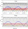 |
Fig. 1 Variation of the gas giant’s eccentricity eGG, under the perturbation of a secondary F-star (top) and M-star (bottom), as a function of time (expressed in T0 units, see text) and for different secondary’s periapsis distance qb. |
The interaction with the disk will be strengthened since the gas giant can encounter a semimajor axis drift. Indeed, we show in Fig. 2 that the dynamical perturbations induced by the secondary can slightly shift the initial semimajor axis of the gas giant inward by a quantity Δ aGG. Therefore, the location of MMRs will be affected since they mainly depend on aGG. The consequences of this type of drift will be analyzed in Sect. 3.3.
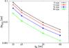 |
Fig. 2 Orbital inward shift Δ aGG of the gas giant as a function of the secondary’s periapsis qb and stellar type. |
3.2. Dynamics of the disk of planetesimals
In Fig. 3, we show the maximum eccentricity reached by the planetesimals at different initial semimajor axes, in the regions ℛ1 and ℛ2 (separated by the dashed vertical line representing the snow-line position). The four panels correspond to the values of qb investigated and each subpanel is for different secondary stellar types (F, G, K, and M). We can distinguish MMRs3 with the gas giant and also a secular resonance: on the bottom panels, which represent the results for ab = 100 au (qb = 70 au and qb = 90 au), we can see a spike located close to or inside the HZ4 (continuous vertical lines) and moving outward (to larger semi-major axes) when increasing the secondary’s mass. This spike represents the secular resonance. When increasing qb, not only does it slightly move inward but also, the maximum eccentricity reached by the particles is higher. This is because the gravitational perturbation from the secondary increases the gas giant’s eccentricity. As a consequence, the forced eccentricity contribution of any particle inside the secular resonance will be increased. When decreasing ab to 50 au (top panels for qb = 35 au and qb = 45 au), the secular resonance moves also outward and reaches the MMR region. As a consequence, the inner disk will suffer from an overlap of these orbital resonances that could cause a fast depletion. However, particles inside the HZ will remain on near circular motion. We should also notice, as studied in detail by Pilat-Lohinger et al. (2016), the combined effects induced by a change of eb when the other dynamical parameters (ab and Mb) remain constant. Indeed, an increase of eb will turn into:
-
an increase of eGG (see Fig. 1) so that the size of the secular perturbed area is increased but the location remains the same;
-
an inward shift of the gas giant with intensity depending on the binary star characteristics (see Fig. 2) where the width of the secular resonance remains unchanged but its location is shifted inward.
As a consequence, only the width (see top panels in Fig. 3) or both the location and the width of the secular resonance can be modified (see bottom panels in Fig. 3), as also shown in Pilat-Lohinger et al. (2016) and Bazsó et al. (2016).
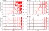 |
Fig. 3 Maximum eccentricity of planetesimals in the ℛ1 and ℛ2 regions, separated by the dashed vertical line for the snow-line position, as a function of their initial position, up to an intermediate integration time of 5 Myr, for different values of qb. Each subpanel refers to the secondary stellar type and the continuous vertical lines refer to the HZ borders. In addition, the inner main MMRs with the gas giant are indicated. |
The outer disk exhibits dynamical outcomes different from the inner disk. Indeed, only external MMRs5 and gravitational interactions with the gas giant perturb ℛ3. As shown in Fig. 1, in the case of qb = 35 au, the periodic high variations of eGG, coupled with the gravitational excitation from the secondary, will cause a strong interaction with the external disk and its dynamical behaviour will be more or less chaotic. When increasing qb (and therefore increasing the size of the disk and decreasing eGG), the external MMRs dominate.
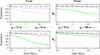 |
Fig. 4 Evolution of the remaining population in the ℛ3 (top) and ℛ2 (bottom) regions according to the periapsis distance qb of a secondary F-type (left) and M-type (right) star. |
To highlight our results, in Fig. 4, we show the dynamical outcome of the ℛ2 and ℛ3 regions for a secondary F-type (left panel) and M-type (right panel) star. Because of the definition of ℛ3, a secondary F-type star at qb = 35 au cannot host an outer disk6. For this value of qb, we can see that more than 80% of the inner disk escaped within 50 Myr. This is because the secular resonance lies inside ℛ2 and its large width (see top right panel in Fig. 3 for the case of a secondary F-type) will favour chaos therein. Thus, this orbital resonance plays an important role for the depletion of a planetesimal disk. We expect similar results for a G- and K-type secondary as the secular resonance lies beyond the snow line. This is not the case for an M-type at the same periapsis distance and we can clearly see that the lack of strong perturbations inside ℛ2 (the secular resonance is inside the snow line, see top right panel in Fig. 3 for the case of a secondary M-type) enables 70% of the inner disk population to survive within 50 Myr. The evolution of the population in ℛ3 will be strongly correlated to this region’s width and to the gravitational interactions with the gas giant and the secondary star. The more compact the outer disk is and the stronger the perturbations are from the massive bodies, the more likely the loss of asteroids in ℛ3.
This result can also put in question the presence and observational evidence of a remaining asteroid belt in these types of systems for ab = 50 au, since an inner disk can suffer from both secular and mean motion perturbations, but also from strong interactions with the gas giant. It might not survive under such conditions since we can observe a linear decrease of the population of ℛ2. Therefore, its dynamical lifetime will vary according to Mb.
3.3. Dynamical lifetime of particles near MMRs
In this section, we investigate in detail the dynamical lifetime of particles which are initially close or inside internal MMRs. They occur when the orbital periods of the gas giant and the particle are in commensurability, such as  where an is the position of the nominal resonance location. As shown in Fig. 2, the gas giant will have periodic variations in the interval [aGG − Δ aGG;aGG]. Thus, for a given pair (p,q), the maximum shift Δ an of an is (p/q)2/3Δ aGG. As we aim to correlate the dynamical lifetime of particles with the binary star characteristics, we preferred to do a separate analysis to ensure that each MMR contains the same number of particles. Indeed, our results would be biased if we were to use the sampling described in Sect. 2. Instead, for each MMR investigated, we defined an interval
  of initial semimajor axis for our test particles:
 ![Mathematical equation: \begin{eqnarray*} \displaystyle \mathcal{A}_{{n}} = \left [a_{n} - \Delta\, a_{ n} - \epsilon;\, a_{n} + \epsilon^\prime \right]\mbox{,}~~~\mbox{} (\epsilon, \epsilon^\prime) \in \mathbb{R,} \end{eqnarray*}](/articles/aa/full_html/2016/07/aa28035-15/aa28035-15-eq58.png) where (ϵ,ϵ′) are arbitrary numbers7 to take into account particles initially orbiting near the MMR and likely to cross it during the integration. We limited this study to resonances with integers p and q ≤ 10. In each MMR, we uniformly distributed 25 particles8 with a step-size that depends on the size of
where (ϵ,ϵ′) are arbitrary numbers7 to take into account particles initially orbiting near the MMR and likely to cross it during the integration. We limited this study to resonances with integers p and q ≤ 10. In each MMR, we uniformly distributed 25 particles8 with a step-size that depends on the size of  , initially on circular and planar orbits. In addition, as suggested by Pilat-Lohinger & Dvorak (2002), each particle is cloned into four starting points with mean anomalies M = 0°, M = 90°, M = 180° and M = 270°, since it is well known that the starting position plays an important role for the dynamical behaviour in MMRs. This accounts for 100 particles in each MMR. Each system was integrated for 50 Myr. We did not consider the condition
  as a criterion for a particle to leave the MMR. Indeed, its dynamical evolution can be quite random: from time to time it can leave an MMR or be temporarily captured into another MMR. Instead, we consider a particle as leaving its initial location in a specific MMR when its dynamical evolution leads to a collision with either one of the stars or the gas giant. Finally, we defined the dynamical lifetime of particles inside a specific MMR as the time required for 50% of the population to leave the resonance (Gladman et al. 1997). In Fig. 5, we show the dynamical lifetime in Myr of particles near the internal MMRs.
 |
Fig. 5 Dynamical lifetime of test particles in ℛ1 and ℛ2 regions expressed in Myr. Top panel: influence of the secondary’s mass when qb = 35 au. Bottom panel: influence of the secondary’s periapsis distance qb assuming the secondary as a G-type star. |
In the top panel of this figure, the influence of Mb is shown for a certain periapsis distance qb = 35 au. The bottom panel summarizes the results for a certain mass of the secondary star (i.e. G-type star) and different periapsis distances of this star. For the top panel, we have chosen qb = 35 au as for this particular value, the secular resonance overlaps with the MMRs in ℛ2. We can see that prior to the 8:3 MMR, the border between icy and rocky asteroids, a secondary M-type will favour chaos inside the rocky bodies region located in ℛ1. This is not surprising since Fig. 3 clearly shows the secular resonance overlapping with MMRs located inside the snow-line at 2.7 au. Beyond this limit, a higher value of Mb leads to a lower dynamical lifetime – values can reach 0.1 Myr – since the secular resonance moves outward. From the bottom panel, one can recognize that the lower qb, the lower the dynamical lifetime. Some MMRs can be quickly emptied within 0.1 Myr. With these tests, we highlight that in binary star systems, the dynamical lifetime of particles initially orbiting inside or close to MMRs can be variable according to the location of the secular resonance. Provided that particles can reach the HZ region before colliding with one of the massive bodies (i.e. the stars or the gas giant) or before being ejected out of the system, they could rapidly cause an early bombardement on any embryos or planets moving in the HZ.
 |
Fig. 6 Represented on the y-axis (left and right axes have the same scale), the variation of the maximum eccentricity (red line) together with the cumulative fraction of water (dashed black line) brought to the HZ, with respect to the initial location of small bodies in ℛ2 and ℛ3. The top panel is for a secondary star at qb = 35 au and the bottom panel is for qb = 45 au. In this figure, is also represented the normalized HZc distribution (blue line) from 0.1 Myr (left) up to 50 Myr (right). The vertical black line refers to the position of the snow line. The entire region ℛ3 is intentionally not displayed because of its size. Instead, only the dynamically interesting part of ℛ3 is shown. |
 |
Fig. 8 Left: influence of the gas giant’s orbital and physical parameters. Top and bottom subpanels are for a secondary F-type and M-type star, respectively. Right: the three subpanels show results for the case of single star systems. Each plot corresponds to an intermediate integration time of 10 Myr. See text in Sect. 5 and legend of Fig. 6 for more details. |
4. Asteroid flux and water transport to the HZ
In this section, we compare the flux of icy particles from ℛ2 and ℛ3 towards the HZ. We recall the definition of habitable zone crossers (HZc) as defined in Paper I. HZc are any particles initially evolving beyond the snow line (2.7 au) and crossing the HZ at least once within the integration time. The authors of Paper I showed that the higher Mb and qb, the more important the rate of HZc and, therefore, the quantity of water transported to the HZ. We analyze here how the orbital resonances influence the asteroid flux to the HZ and the amount of water borne therein. On the y-axis in Fig. 6, we represent the evolution of the maximum eccentricity (red line) of particles inside ℛ1, ℛ2 (as already drawn in Fig. 3) and ℛ3. The top panel corresponds to a secondary star at qb = 35 au and the bottom panel is for qb = 45 au, each subpanel corresponding either to a secondary F- or M-type star. We chose these two cases to highlight the impact of the location of the secular resonance when it lies inside the snow line (M-type) and beyond the snow line (F-type). From left to right, each figure is for a different period of integration (between 0.1 Myr to 50 Myr). We also show the normalized HZc distribution (blue line) calculated regarding the total number of HZc produced by the corresponding systems for each period of integration time. For all cases considered, within 10 Myr, the 2:1 MMR located at ~3.28 au and the secular resonance, when it lies beyond the snow line, are the primary sources of HZc in the inner disk. In addition, the external disk can produce a non-negligible or equivalent number of HZc, compared to the inner disk. Indeed, as mentioned in Sect. 2, the smaller is qb the more compact is the outer disk. In this case, the depletion can be fast and the dynamics are more chaotic. As a result, asteroids might not cross the HZ before colliding with the stars and the gas giant or being ejected. To estimate the amount of transported water, we followed the same approach as in Paper I, i.e. the contribution of the maximum water content of all the HZc when they first cross the HZ. On the same figure, the y-axis also corresponds to the cumulative fraction of water (dashed black line) brought by the HZc. This fraction is determined with respect to the final amount of transported water from ℛ2 and ℛ3 within 50 Myr. As already mentioned in Sect. 2, a system with an F-star as a companion and qb = 35 au cannot host an outer disk. Therefore, all the incoming water in the HZ for this particular system is from ℛ2. All our systems exhibit the same trend: the quantity of incoming water inside the HZ drastically increases when particles orbit initially inside the secular resonance and the 2:1 MMR. We show similar results in Fig. 7 for qb = 70 au (top panel) and qb = 90 au (bottom panel). Contrary to the previous case, the secular resonance does not contribute at all to bearing water material into the HZ since it lies in this region (see Fig. 3). We show that the two main sources of HZc in ℛ2 are the 2:1 and 5:3 MMR. The contribution of ℛ3 is more negligible than in the previous case since its size is more extended and weakly perturbed.
5. Influence of the dynamical parameters on the planetesimal disk
We are interested in how the previous results, mainly the origin of HZc and the water transport to the HZ, are influenced by the gas giant’s dynamical and physical parameters and when, considering the case of one or two gas giants that orbit a single star. The same number of particles were placed in the three regions9 as defined in Sect. 2, but we did not repeat the simulations for all the binary systems investigated in the previous sections. Instead, we selected two for comparison: a secondary F-type with qb = 45 au and a secondary M-type with qb = 70 au. Thus, a comparison of the results from this section and illustrated in Fig. 8 is made in the bottom panels of Fig. 6 (top figure for the F-type) and top panels in Fig. 7 (bottom figure for the M-type). The results shown in Fig. 8 correspond only to 10 Myr of integration time.
5.1. Gas giant’s orbital and physical parameters
We investigated different cases to separately highlight the influence of the initial parameters aGG, eGG, and MGG. The results are shown on the left panels in Fig. 8:
-
Case 1 (top panel): we increase the initial eccentricity toeGG = 0.2. For both cases (F- and M-types), the participation of ℛ2 in the water transport to the HZ is much more important than ℛ3, since region ℛ2 is mainly dominated by chaos. Indeed, in addition to stronger interactions with the disk, the width of the secular resonance will be increased, for the case of the secondary F-type star, as pointed out in Pilat-Lohinger et al. (2016). Both strong mechanisms explain the higher flux of asteroids towards the HZ in comparison with eGG = 0.0.
-
Case 2 (middle panel): we change the initial gas giant’s semimajor axis to aGG = 4.5 au and 6.0 au. As a consequence, the secular resonance will be shifted inward or outward respectively. For a secondary F-type, for instance, the semi-analytical method developed by Pilat-Lohinger et al. (2016) predicts an inward shift close to the 5:2 MMR (inside the snow-line) or an outward shift beyond the 2:1 MMR, respectively. Furthermore, in both cases (F- and M-types), decreasing aGG to 4.5 au results in shifting the 5:2 MMR inside ℛ1 (therefore it will not participate in bearing water to the HZ), whereas increasing aGG to 6.0 au results in shifting the 3:1 MMR inside ℛ2 (thus it participates in moving icy asteroids from beyond the snow line to the HZ region).
-
Case 3 (bottom panel): we change the mass of the gas giant to MGG = 3MJ and MJ/ 3. In the case of a secondary F-type star, for instance, the theoretical location of the secular resonance is shifted inward for MGG = 3MJ (the secular resonance is below the 3:1 MMR) and outward for MGG = MJ/ 3. For both secondaries (F- and M-types), the MMRs produce a significant amount of HZc within 0.1 Myr for MGG = 3MJ and 10 Myr for MGG = MJ/ 3 whereas 1 Myr is needed for MGG = 1MJ.
5.2. Single star case
In case only one star is present in the system, we aim to compare the previous results with the case of one or two giant planets orbiting a G2V star. We study three possibilities for the giant planets’ configurations and the corresponding results are shown in the right panels of Fig. 8:
-
Case 1 (top panel): one Jupiter at 5.2 au initially on a circular orbit.
-
Case 2 (middle panel): one Jupiter at 5.2 au initially on an elliptic orbit with eGG = 0.2.
-
Case 3 (bottom panel): a system with two giant planets, i.e. a Jupiter and a Saturn10.
For the three cases, the value of the outer border of ℛ3 is equal to the highest value of ac in Table 1 (i.e. a wide outer disk). The value of the inner border of ℛ3 is calculated taking into account the Hill radius of the outer giant planet (i.e. the Jupiter-like for one gas giant and the Saturn-like if the system contains two gas giants). Unsurprisingly, because of the lack of strong perturbations11, only small bodies initially orbiting close to the gas giant can become HZc (case 1). The flux of icy asteroids drastically increases as soon as the initial eccentricity of the gas giant is increased (case 2): the interaction with the disk is stronger and it is not easy to identify the most efficient MMR that is producing HZc but the region ℛ2 is the main source of water. In contrast, the contribution of ℛ3 in case 3 is as important for ℛ2 because of the presence of the second gas giant. Contrary to the binary cases in which the 2:1 MMR and the secular resonance (when lying inside ℛ2, see Fig. 6) were the primary sources of HZc within the whole integration time, in case 3, the 2:1 MMR becomes dominant only within 10 Myr of integration. Below 10 Myr, the 5:2 and 5:3 MMRs dominate over the other MMRs.
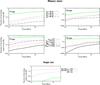 |
Fig. 9 Fraction of incoming water in the HZ with respect to the initial total amount of water in the disk of planetesimals, considering various configurations. Top and middle panels show results in binary star systems for fixed and variable values of the gas giant’s orbital and physical parameters, respectively, when the secondary is an F-type (left) and M-type (right) star (see text in Sect. 5.1). Comparison with various single star systems are shown in the bottom panel (see text in Sect. 5.2). |
6. Comparison of the water transport efficiency
Finally, in Fig. 9, we combine the results obtained in Sects. 4 and 5 to compare the total amount of water transported into the HZ, expressed with respect to the initial total amount of water in the disk. The top panel compiles the results obtained in Sect. 4 for a secondary F-type (left) and M-type (right). The middle panel compiles the results from Sect. 5.1 when changing the gas giant’s orbital and physical parameters, for a secondary F-type at qb = 45 au and a secondary M-type at qb = 70 au. Finally, the bottom panel shows the results for single star systems containing one or two gas giants.
In the binary cases, when the parameters of the gas giant are fixed (top panels), one can see for instance, that a secondary M-type star at qb = 35 au, needs ~50 Myr so that one quarter of the water initially in the disk of planetesimals is transported to the HZ, contrary to an F-type star where only ~0.5 Myr is needed. This is mainly due to the presence of the secular resonance inside the asteroid belt in ℛ2.
When changing the gas giant’s orbital and physical parameters (middle panels), the water transport efficiency to the HZ can be different (comparisons have to be made with the red-dashed line for the secondary F-star at qb = 45 au and the blue-dotted line for the M-type at qb = 70 au in the top panels). For instance, the figure reveals that increasing eGG boosts the water transport efficiency. Indeed, within 0.1 Myr, almost 50% of the initial water ended up in the HZ in the case of an F-star, and nearly 20% for an M-type12. When changing aGG, even with the lack of active orbital resonances in the case of aGG = 4.5 au (the 5:2 MMR and the secular resonance lie inside the snow-line), the 2:1 and 5:3 MMR are powerful enough so that the water transport is as efficient as for a giant planet at aGG = 5.2 au. For aGG = 6.0 au, since the 3:1 MMR participates in the asteroid flux, the water transport is even more efficient. The mass of the gas giant also influences the final total amount of water brought to the HZ as a higher or smaller value of MGG, respectively, strengthens or weakens the water transport efficiency of a binary star system.
Finally, comparable results (bottom panel) can be obtained with different single star configurations hosting either one or two giants planets. If only one giant planet, with eGG = 0.0, orbits a sun-like star, a significant water transport in the HZ within 50 Myr is very unlikely because of the lack of gravitational perturbations. However, if the gas giant initially starts on an eccentric orbit (eGG = 0.2), the depletion of ℛ2 is quite fast and within 0.1 Myr, the water transport efficiency can be comparable to a secondary F-type star at qGG = 45 au within 50 Myr. This is not surprising since such a high eccentricity favours chaos in ℛ2. Last but not least, if two giant planets (Jupiter- and Saturn-like) orbit a sun-like star, both regions ℛ2 and ℛ3 are water sources since several inner and outer MMRs with the giant planets are active and 50 Myr are needed to transport 10% of the water initially present in the disk. These results are comparable to the binary star systems simulations with an M-type as a companion.
7. Conclusion
We showed that the flux of icy bodies towards circumprimary HZs in binary star systems can vary according to the characteristics and motion of the secondary star and the giant planet. First, we showed that a gas giant planet can suffer from both variations of its orbital eccentricity and a drift in semi-major axis. This in turn could strengthen the interaction with an inner (region ℛ2) and outer (region ℛ3) disk of planetesimals. Moreover we highlight that in tight binaries (ab = 50 au), a secular resonance can lie within the inner asteroid belt, overlapping with MMRs, which enable, in a short timescale, an efficient and significant flux of icy asteroids towards the HZ, in which particles orbit in a near circular motion (region ℛ1). By way of contrast, in the study of wide binaries (ab = 100 au), particles inside the HZ can move on eccentric orbits when the secular resonance lies in the HZ. The outer asteroid belt is only perturbed by MMRs. As a consequence, a longer timescale is needed to produce a significant flux of icy asteroids towards the HZ. These dynamics drastically impact the dynamical lifetime of particles initially located inside inner MMRs. Indeed, this can range from thousands of years to several million years according to the location of the MMR within the secular resonance. This can favour a fast and significant contribution of MMRs in producing HZc, which are asteroids with orbits crossing the HZ and bearing water therein. In any case, we highlighted that, for the studied binary star systems, the inner disk (region ℛ2) is the primary source of HZc (and therefore water in the HZ), by means of the 2:1 MMR, the 5:3 MMR, and the secular resonance, when this latter lies close or beyond the snow line. As shown in Sect. 5.1, the gas giant’s characteristics also influence the asteroids flux to the HZ and therefore the water transport. Indeed, the dynamical interactions can be different since the location of the orbital resonances can be shifted inward or outward. Giant planets, initially on eccentric orbits, are an efficient way to ensure that the HZ can be rapidly fed with water (within 0.1 Myr) since it can increase the width of the secular resonance for instance. Even gas giants with lower mass can be efficient in the water transport to the HZ but on a longer timescale. For any giant planet configuration studied, the 2:1 MMR and 5:3 MMR also appeared to be powerful perturbations for transporting water into the HZ. This is not necessarily the case in single star systems. In Jupiter- and Saturn-like systems orbiting a sun-like star, other inner and outer MMRs are also, to a lesser extent, water sources.
As for the amount of transported water that effectively ends up on embryos and planets in the HZ, both Fig. 3 and Paper I have pointed out two opposite behaviours that depend on the binary’s orbit: a high rate of HZc and nearly circular motion in the HZ (tight binary) versus low rate of HZc and eccentric orbits in the HZ (wide binary). The main problems of the tight-binary case are:
-
a)
planets or embryos moving on nearly circular motion in the HZhave lower impact probabilities with HZc – with regard also to thewater distribution within the HZ as shown inPaper I – than if they were moving on eccentricorbits;
-
b)
the asteroid flux to the HZ is a fast process. If the primary star is in the T-Tauri phase, Tu et al. (2015) show that the activity of a present Sun-like star can have a different history because of its rotational behaviour. As a consequence, planetary embryos might not be able to keep the incoming water on their surface;
-
c)
with respect to this last point, and that the depletion of the inner disk (region ℛ2) can be quite fast, there would not be other water sources available after the activity of the primary star has significantly decreased, if the remaining asteroids (in the inner and outer disk) stay on stable orbits.
In wide binaries, since the flux process is much slower, the activity of a young primary star would not be an obstacle for a planet to keep the water borne from asteroids on its surface, even if it loses its primary surface water content. Indeed, the eccentric motion inside the HZ can have a positive aspect: since planetary embryos can leave the HZ from time to time, they can increase their impact probabilities since they can also interact with icy asteroids evolving beyond the outer border of the HZ. However, the
high eccentric motion inside the HZ can also raise some problems that would be subject to future study.
The numerical value is T0 = 6323 yr.
The difference does not exceed ~0.5%.
Only the main ones are indicated.
The borders are defined according to Kopparapu et al. (2013).
MMRs with the secondary star also influence the dynamics of celestial bodies and their location depends on the secondary star’s orbital parameters. However, they have a very high order and their contribution is much weaker compared to the MMRs with the gas giant.
as ac – Δac≤aGG + 3 RH,GG.
(ϵ,ϵ′) ~ ± 1%.
We did not put more particles as is very narrow. In ℛ2, the size of is ~ Δ an ≤ Δ aGG as (p/q)2/3 ≤ 1. In ℛ3, we would have considerered an other approach as the size of would be much wider because (p/q)2/3 ≥ 1.
The size of ℛ2 and ℛ3 can vary because of RH,GG.
Their mass and initial orbital elements are the commonly used ones.
There cannot be a secular resonance; only MMRs can perturb the asteroids’ orbits
For both cases, this is 2.5 times more than for the case eGG = 0.
Acknowledgments
D.B. and E.P.L. acknowledge the support of the Austrian Science Fundation (FWF) NFN project: Pathways to Habitability, subproject S11608-N16 Binary Star Systems and Habitability. D.B. and E.P.L. acknowledge also the Vienna Scientific Cluster (VSC project 70320) for computational resources. A.B. and E.P.L. acknowledge the support of the FWF project P22603-N16.
References
- Bancelin, D., Pilat-Lohinger, E., Eggl, S., et al. 2015, A&A, 581, A46 [NASA ADS] [CrossRef] [EDP Sciences] [Google Scholar]
- Bazsó, Á., Pilat-Lohinger, E., Eggl, S., Funk, B., & Bancelin, D. 2016, ArXiv e-prints [arXiv:1605.06769] [Google Scholar]
- Briceño, C., Vivas, A. K., Calvet, N., et al. 2001, Science, 291, 93 [NASA ADS] [CrossRef] [Google Scholar]
- Chambers, J. E. 1999, MNRAS, 304, 793 [NASA ADS] [CrossRef] [MathSciNet] [Google Scholar]
- Gladman, B. J., Migliorini, F., Morbidelli, A., et al. 1997, Science, 277, 197 [NASA ADS] [CrossRef] [Google Scholar]
- Gomes, R., Levison, H. F., Tsiganis, K., & Morbidelli, A. 2005, Nature, 435, 466 [NASA ADS] [CrossRef] [PubMed] [Google Scholar]
- Haghighipour, N., & Raymond, S. N. 2007, ApJ, 666, 436 [NASA ADS] [CrossRef] [Google Scholar]
- Holman, M. J., & Wiegert, P. A. 1999, AJ, 117, 621 [NASA ADS] [CrossRef] [Google Scholar]
- Kopparapu, R. K., Ramirez, R., Kasting, J. F., et al. 2013, ApJ, 765, 131 [NASA ADS] [CrossRef] [Google Scholar]
- Morbidelli, A., Chambers, J., Lunine, J. I., et al. 2000, Met. Planet. Sci., 35, 1309 [Google Scholar]
- Mudryk, L. R., & Wu, Y. 2006, ApJ, 639, 423 [NASA ADS] [CrossRef] [Google Scholar]
- Murray, C. D., & Dermott, S. F. 1999, Solar system dynamics (CUP) [Google Scholar]
- O’Brien, D. P., Walsh, K. J., Morbidelli, A., Raymond, S. N., & Mandell, A. M. 2014, Icarus, 239, 74 [NASA ADS] [CrossRef] [Google Scholar]
- Pilat-Lohinger, E. 2005, in Dynamics of Populations of Planetary System, eds. Z. Knežević, & A. Milani, IAU Colloq., 197, 71 [Google Scholar]
- Pilat-Lohinger, E., & Dvorak, R. 2002, Celest. Mech. Dyn. Astron., 82, 143 [Google Scholar]
- Pilat-Lohinger, E., Süli, Á., Robutel, P., & Freistetter, F. 2008, ApJ, 681, 1639 [NASA ADS] [CrossRef] [Google Scholar]
- Pilat-Lohinger, E., Bazso, A., & Funk, B. 2016, ArXiv e-prints [arXiv:1605.07359] [Google Scholar]
- Rabl, G., & Dvorak, R. 1988, A&A, 191, 385 [NASA ADS] [Google Scholar]
- Thebault, P., & Haghighipour, N. 2014, ArXiv e-prints [arXiv:1406.1357] [Google Scholar]
- Tsiganis, K., Gomes, R., Morbidelli, A., & Levison, H. F. 2005, Nature, 435, 459 [NASA ADS] [CrossRef] [PubMed] [Google Scholar]
- Tu, L., Johnstone, C. P., Güdel, M., & Lammer, H. 2015, A&A, 577, L3 [NASA ADS] [CrossRef] [EDP Sciences] [Google Scholar]
- Walsh, K. J., Morbidelli, A., Raymond, S. N., O’Brien, D. P., & Mandell, A. M. 2011, Nature, 475, 206 [NASA ADS] [CrossRef] [PubMed] [Google Scholar]
All Tables
All Figures
|
Fig. 1 Variation of the gas giant’s eccentricity eGG, under the perturbation of a secondary F-star (top) and M-star (bottom), as a function of time (expressed in T0 units, see text) and for different secondary’s periapsis distance qb. |
| In the text | |
|
Fig. 2 Orbital inward shift Δ aGG of the gas giant as a function of the secondary’s periapsis qb and stellar type. |
| In the text | |
|
Fig. 3 Maximum eccentricity of planetesimals in the ℛ1 and ℛ2 regions, separated by the dashed vertical line for the snow-line position, as a function of their initial position, up to an intermediate integration time of 5 Myr, for different values of qb. Each subpanel refers to the secondary stellar type and the continuous vertical lines refer to the HZ borders. In addition, the inner main MMRs with the gas giant are indicated. |
| In the text | |
|
Fig. 4 Evolution of the remaining population in the ℛ3 (top) and ℛ2 (bottom) regions according to the periapsis distance qb of a secondary F-type (left) and M-type (right) star. |
| In the text | |
|
Fig. 5 Dynamical lifetime of test particles in ℛ1 and ℛ2 regions expressed in Myr. Top panel: influence of the secondary’s mass when qb = 35 au. Bottom panel: influence of the secondary’s periapsis distance qb assuming the secondary as a G-type star. |
| In the text | |
|
Fig. 6 Represented on the y-axis (left and right axes have the same scale), the variation of the maximum eccentricity (red line) together with the cumulative fraction of water (dashed black line) brought to the HZ, with respect to the initial location of small bodies in ℛ2 and ℛ3. The top panel is for a secondary star at qb = 35 au and the bottom panel is for qb = 45 au. In this figure, is also represented the normalized HZc distribution (blue line) from 0.1 Myr (left) up to 50 Myr (right). The vertical black line refers to the position of the snow line. The entire region ℛ3 is intentionally not displayed because of its size. Instead, only the dynamically interesting part of ℛ3 is shown. |
| In the text | |
 |
Fig. 7 Same as for Fig. 6 but for qb = 70 au (top panel) and qb = 90 au (bottom panel). |
| In the text | |
|
Fig. 8 Left: influence of the gas giant’s orbital and physical parameters. Top and bottom subpanels are for a secondary F-type and M-type star, respectively. Right: the three subpanels show results for the case of single star systems. Each plot corresponds to an intermediate integration time of 10 Myr. See text in Sect. 5 and legend of Fig. 6 for more details. |
| In the text | |
|
Fig. 9 Fraction of incoming water in the HZ with respect to the initial total amount of water in the disk of planetesimals, considering various configurations. Top and middle panels show results in binary star systems for fixed and variable values of the gas giant’s orbital and physical parameters, respectively, when the secondary is an F-type (left) and M-type (right) star (see text in Sect. 5.1). Comparison with various single star systems are shown in the bottom panel (see text in Sect. 5.2). |
| In the text | |
Current usage metrics show cumulative count of Article Views (full-text article views including HTML views, PDF and ePub downloads, according to the available data) and Abstracts Views on Vision4Press platform.
Data correspond to usage on the plateform after 2015. The current usage metrics is available 48-96 hours after online publication and is updated daily on week days.
Initial download of the metrics may take a while.