| Issue |
A&A
Volume 591, July 2016
|
|
|---|---|---|
| Article Number | A19 | |
| Number of page(s) | 9 | |
| Section | Interstellar and circumstellar matter | |
| DOI | https://doi.org/10.1051/0004-6361/201527803 | |
| Published online | 06 June 2016 | |
CN Zeeman and dust polarization in a high-mass cold clump⋆
Max-Planck-Institut für Radioastronomie, Auf dem Hügel, 53121 Bonn, Germany
e-mail: This email address is being protected from spambots. You need JavaScript enabled to view it.
Received: 21 November 2015
Accepted: 16 February 2016
Abstract
We report on the young massive clump (G35.20w) in W48 that previous molecular line and dust observations have revealed to be in the very early stages of star formation. Based on virial analysis, we find that a strong field of 1640 μG is required to keep the clump in pressure equilibrium. We performed a deep Zeeman effect measurement of the 113 GHz CN (1−0) line towards this clump with the IRAM 30 m telescope. We combine simultaneous fitting of all CN hyperfines with Monte Carlo simulations for a large range in realization of the magnetic field to obtain a constraint on the line-of-sight field strength of −687 ± 420 μG. We also analyze archival dust polarization observations towards G35.20w. A strong magnetic field is implied by the remarkably ordered field orientation that is perpendicular to the longest axis of the clump. Based on this, we also estimate the plane-of-sky component of the magnetic field to be ~740 μG. This allows for a unique comparison of the two orthogonal measurements of magnetic field strength of the same region and at similar spatial scales. The expected total field strength shows no significant conflict between the observed field and that required for pressure equilibrium. By producing a probability distribution for a large range in field geometries, we show that plane-of-sky projections are much closer to the true field strengths than line-of-sight projections. This can present a significant challenge for Zeeman measurements of magnetized structures, even with ALMA. We also show that CN molecule does not suffer from depletion on the observed scales in the predominantly cold and highly deuterated core in an early stage of high-mass star formation and is thus a good tracer of the dense gas.
Key words: ISM: magnetic fields / ISM: clouds / stars: protostars / magnetic fields / methods: observational / techniques: polarimetric
Based on observations carried out with the IRAM 30 m Telescope. IRAM is supported by INSU/CNRS (France), MPG (Germany) and IGN (Spain).
© ESO, 2016
1. Introduction
High-mass stars (≥8 M⊙) exhaust lighter elements and initiate carbon fusion. The mass functions of stellar populations in widely different environments reveals that such stars are far fewer in number than low-mass stars (Zinnecker & Yorke 2007). Yet, they manage to dominate the interstellar medium (ISM) energetics and influence the galaxy as a whole throughout their evolution. Therefore it is important to understand how these stars form; indeed, there have been tremendous strides in the field of high-mass star formation in the last decade. Multi-wavelength surveys of the whole or large parts of the Galactic plane, followed up by targeted observations in the last decade have revolutionized our understanding of their formation (see Tan et al. 2014). Such studies have revealed that typical high-mass protostellar cores are highly Jeans unstable. Therefore, theoretically turbulence is expected to have a significant influence in forming high-mass stars (McKee & Tan 2002). Observations of high-mass star-forming regions show supersonic line widths in molecular gas tracers supporting this scenario. Magnetic fields may be equally important in such regions. However, direct measurements of line-of-sight (los) magnetic fields appear to show that such regions are magnetically super-critical and thus, do not favor this scenario (see Crutcher 2012). However these measurements generally have targeted clumps that contain already formed stars whose feedback might have altered the initial properties.
Largely unexplored however, are the initial conditions of high-mass star formation. Pristine prestellar clumps may be found in the vicinity of very young high-mass protostars (with little feedback effects), which should represent such initial conditions with material in a cold (10−20 K) and quiescent phase. There is therefore considerable current interest in the study of such high-mass clumps. Recently, a few studies have been conducted at high resolution, involving a one-to-one comparison of mass derived from observations of thermal dust continuum and virial mass, to understand whether such clumps are in virial equilibrium (Pillai et al. 2011; Kauffmann et al. 2013; Tan et al. 2013). Such studies find that the most massive clumps are unstable to collapse, unless an enhanced background magnetic field (≥500 μG) exists. Given this, a determination of the magnetic field strength in these sources is highly desirable.
Data summary.
In contrast with parameters like density, temperature, velocity field, and molecular abundances, it has been notoriously difficult to measure B-fields in any regime of the ISM from diffuse clouds to dense star-forming cores (see Crutcher 2012; Li et al. 2014). The two main methods to determine magnetic field strength are dust polarization and Zeeman measurements. Dust polarization measurements along with velocity dispersions can be used to determine the B-field by gauging the dispersion in the polarization vectors. A more direct method of measuring the field strength B is via the Zeeman effect, which causes a frequency shift between the left-hand and right-hand circularly polarized components of a spectral line with a suitable electronic structure. CN is one such molecular gas tracer, whose ground-state hyperfine structure (hfs) transitions near 113 GHz can be detected in clouds with densities ≥a few 104 cm-3. This density regime is the most crucial for the onset of star formation. The Zeeman signal however is exceedingly weak, making its detection extremely difficult, even for relatively strong lines. Therefore, all CN detections to date have been made in very active high-mass star-forming regions with evolved high-mass protostars that have bright lines, and strong fields (Crutcher 1999; Falgarone et al. 2008).
Here, we present magnetic field observations of a very young high-mass clump. The observations include Zeeman measurements from the IRAM 30 m telescope and archival dust polarization observations. The target selection and observations are detailed in Sects. 2 and 3, respectively. Zeeman data reduction and analysis followed by results from the polarization data are reported in Sect. 4.
2. The target: G35.20w
Our Zeeman target G35.20w (see Fig. 1) lies about 1′ west of the W48 Hii region (G35.20−1.74). We adopt a distance of 3.27 kpc based on trigonometric maser parallax measurements toward G35.20-1.74 (Zhang et al. 2009). The dust polarization data has been published by Curran et al. (2004) where our target is identified as W48W. Our interferometer 3 mm dust continuum and NH2D observations have revealed that the clump consists of several massive (120 M⊙ on average) and cold cores. Pillai et al. (2011) find these cores to be highly supercritical. The region is infrared quiet except for the most massive core, which hosts an embedded protostar driving a massive outflow (Pillai et al. 2011, hereafter P11). The derived core masses exceed the mass-size threshold for high-mass star formation (Kauffmann & Pillai 2010; Kauffmann et al. 2010) by at least a factor of 10. The clump is characterized by high deuteration and low gas temperatures ~20 K derived from NH3 measurements of P11. The extreme youth of the clump is further confirmed by Rygl et al. (2014) who show that the cold cores in this region are dense structures with the lowest dust temperature (<20 K) of the whole W48A environment; these authors base their findings on Herschel dust temperature and column density measurements. Rygl et al. also derive a bolometric luminosity of 4000 L⊙ (Clump H3 in their terminology) with an estimated age of <0.2 Myr. Thus, all observations point to G35.20w being a massive star-forming clump in its youngest stage of evolution.
SCUBA dust continuum data centered on G35.20w is represented in Fig. 1. A summary of the data discussed in this paper is given in Table 1.
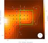 |
Fig. 1 G35.20w SCUBA archival 850 μm polarization vectors rotated by 90° to show the magnetic field orientation, overlaid on SCUBA 850 μm dust continuum archival data (color scale). The position offsets are w.r.t. the coordinates given in Table 1. The box shows the region around our IRAM 30 m CN observations to which we confine our analysis. Polarization data is only shown where the polarization level is ≥3σ, corresponding to an uncertainty in position angle ≤9.5°. The length of the Bpos vector represents the percentage of polarization. |
3. Observations
3.1. IRAM 30 m Zeeman observations
We started with pointed observations toward G35.20w in the CN N = 1−0 line at 113 GHz with the IRAM 30 m telescope. Then, we performed a five-point map around the peak. The beam at this frequency is 23.5′′ (FWHM). In Table 2, we give the frequencies of the relevant hfs transitions that have significant Zeeman splitting (N = 1−0 transition). After reducing this data, we concluded that the submm clump is characterized well by the CN emission (see Sect. 4.2) and that the optical depth of CN hyperfine structure (hfs) components is moderate enough to allow for a reliable Zeeman fitting. We carried out the Zeeman observations with the XPOL setup (Thum et al. 2008) over several days in April to May 2010 in good 3 mm weather conditions (2−3 mm water vapor). The final rms on the peak position is 6 mK. The data were analyzed in CLASS1.
CN N = 1−0 transitions with significant Zeeman splitting.
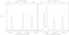 |
Fig. 2 CN(N = 1 → 0,J = 1/2 → 1/2) (left) and J = 1/2 → 3/2 (right) spectrum toward G35.20w. The LSR velocity is shown with respect to the component at 113 499.64 MHz (red dashed line). |
3.2. SCUBA archival dust polarization observations
Thompson et al. (2005) reported the SCUBA observations that resulted in our dust continuum data. We also analyze archival calibrated polarization data obtained with the SCUBA instrument at the JCMT. Specifically, we use data from the SCUPOL catalog, which is a compilation of 850 μm polarization observations at JCMT (Matthews et al. 2009). We refer to Matthews et al. for a description of the observations and data reduction. Data for G35.20w has already been published by Curran et al. (2004). They derive a magnetic field strength and assess the mass-to-flux ratio using the Chandrasekhar-Fermi method, however with a highly uncertain mass estimate and an assumed velocity dispersion. With temperature, density and velocity dispersion measurements from our previous work at high as well as low resolution (P11), we are now able to obtain as accurate an estimate of the field strength as possible.
4. Results
4.1. Dense clump properties
Here, we revisit the P11 results for G35.20w. We recalculate the parameters of the clump now extracted only toward the region around our IRAM 30 m CN observations. We have thus chosen to exclude the secondary peaks detected in our larger dust continuum image. The region thus confined is shown as a green box in Fig. 1. We extract the total flux within that region from SCUBA dust continuum observations at 850 μm to determine the total mass. The virial mass is characterized by the line width (2.1 km s-1) associated with the systemic velocity component (42.4 km s-1) over the same region using our CN observations following the formulation in P11. The effective radius estimated from the source area A (green box in Fig. 1) calculated as  is ~0.35 pc. We derive a virial mass of 347 M⊙. The average gas temperature from previous NH3 observations is 20 K (P11). Assuming the same temperature for dust as confirmed by Rygl et al. (2014) and a dust opacity of 0.02 cm2/g (Ossenkopf & Henning 1994; thin ice mantles at n(H) = 106 cm-3), we derive a mass of 1650 M⊙ following Kauffmann et al. (2008). For reference, the parameters extracted for the region are also listed in Table 3.
4.2. CN Zeeman results
In Fig. 2, we show our CN spectrum toward G35.20w. A single velocity component yields a poor fit to the hyperfine spectrum. The brightest component at 113 488.12 GHz (line 4) is partially blended with the component at 113 490.97 GHz (line 5). Excluding these components, we stack the other hyperfine components and perform multiple component Gaussian fits (see next section).
Although the CN 1−0 transition has already been used to measure B-fields in active high-mass regions (Crutcher et al. 2010), it has been unclear whether this transition is a selective photodissociation region (PDR) tracer or rather a dense gas tracer in star-forming regions. A recent wide-field interferometer mapping in the dense molecular envelope of the ultracompact HII region W3OH, however, finds that CN is an excellent tracer of warm high density gas (Hakobian & Crutcher 2011). Maury et al. (2012) show that in NGC 2264-C, an intermediate-mass protocluster without significant ionizing radiation in its vicinity, the CN emission closely follows the dust continuum emission. In Fig. 3, an integrated intensity map of CN for the main hyperfine component is shown with respect to the SCUBA 850 μm dust continuum emission. The dust continuum emission within the field of view (FOV) shows a bright core at x, y-offset + 60′′, −10′′ (the well-known W48 UCHii region) as well as a secondary core [at (0, 0)] that is our target (G35.20w). The CN emission shows a compact peak at the 30 m pointing center and a structure that correlates well with the dust emission as shown in the correlation plot in Fig. 3 (right panel).
 |
Fig. 3 Left: SCUBA 850 μm dust continuum archival data (colorscale) and CN intensity integrated over the 113 170.49 MHz hyperfine from 34 to 42 km s-1 (contours, 1.2 to 4 in steps of 0.3 K km s-1). The offsets positions for the CN map and the IRAM 30 m beam are shown as black squares and dashed circle respectively. Right: correlation plot of 850 μm flux (smoothed to 23.5′′) and CN integrated intensity. |
In Fig. 4, we show the final Stokes V spectrum obtained as a weighted average of all Zeeman–sensitive transitions. In spite of the deep observations with very good 3 mm conditions, we do not detect a significant Stokes V component. The final rms is 4.6 mK for a 0.1 km s-1 velocity resolution for a telescope time of ~33 h.
4.2.1. CN 1−0 hyperfine fitting and optically depth
In the following subsection, we discuss a new method to fit the CN hfs components robustly and simultaneously. We stack all the hyperfine components except the blended lines (4 and 5 in Table 2) and obtain a best fit with two velocity components. A two-component fit provides a good fit to the hfs components with one narrow component (~2.1 km s-1 FWHM), with a peak brightness of 1.18 K centered at the systemic source velocity (42.5 km s-1, see P11), and a weaker (0.46 K), wide (~5.0 km s-1 FWHM) and likely diffuse component at ~42.0 km s-1. We assume that it is the component at the systemic velocity that is associated with the dense gas and hence higher field strength that contributes to the Zeeman splitting. The fit parameters (line width and velocity) are then saved into an initialization file where the line width and velocity of the diffuse component is fixed. The input file for our Zeeman analysis (next Sect. 4.2.2) has the following parts. The first part is obtained after we stack all the hfs components together and perform two velocity component fits to the stacked spectrum. We subtract both fits in the Stokes I data based on the initialization file. The second part is obtained similarly, except that we only subtract the diffuse feature at ~42.0 km s-1, where the residual Stokes I spectra is left with the systemic velocity feature (~42.5 km s-1). Finally, the original Stokes I and Stokes V are included as the third and fourth part.
Our approach to the Zeeman analysis relies on the assumption that the emission of all the hfs components is optically thin. Previous CN 1−0 observations in even more evolved regions confirm that the emission is optically thin (Falgarone et al. 2008). The deviation of the relative intensity of the hfs components from local thermodynamic equilibrium (LTE) is a measure of the optical depth. Following Table 1 of Falgarone et al. (2008), for optically thick emission, the ratio of line intensities for lines 6 and 7 with respect to line 5 is expected to be 1, while for small optical depths, the expected ratio is 3.4. Since the observed ratio of 2.1 is intermediate to these values, we conclude that the optical depth is moderate. From the simultaneous hfs component fit in CLASS, we also find that the optical depth for the brightest hfs components (which we exclude from our analysis) is at most 1.4, while the weaker components have τ ≪ 1. Therefore, we proceed with the assumption that the emission is in LTE.
4.2.2. CN Zeeman fitting
We follow Crutcher et al. (1996) to fit the Zeeman signal in our spectra. The velocity-dependent Stokes I(v) and V(v) signals of the 1–0 transition of CN can be understood as a sum of seven hfs components. These are indicated as Ii and Vi in the following. Crutcher et al. assume that Vi can be modeled as 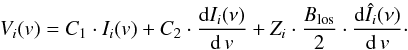 (1)The factors dIi(ν)/d v and dÎi(ν)/d v in this relation give the first derivative of the spectra with respect to frequency. The Zeeman splitting factors are given by the Zi. We obtain Îi by subtracting unrelated velocity components from the spectra Ii, as described above.
The first term in Eq. (1) describes the instrumental, quasi-achromatic leakage of Stokes I into Stokes V. The second term accounts for artificial Zeeman features that arise when a velocity gradient is seen by an anti-symmetric beam pattern in Stokes V, for example, owing to a beam squint. Thum et al. (2008) provide some typical beam shapes for different Stokes parameters. The last term is proportional to the magnetic flux density projected along the los, Blos. It describes the signal caused by the Zeeman effect. A simultaneous fit of several hfs components in Stokes Ii and Vi therefore, allows us to separate the true Zeeman signal in the spectra from instrumental bias. For Zi, we refer to Table 2 (adapted from Falgarone et al. 2008). This method assumes that a velocity gradient if any is identical for both velocity components. Given that the large scale component is much weaker and broader than the feature at the systemic velocity (see Sect. 4.2.1), this is a valid assumption.
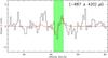 |
Fig. 4 Weighted average of all Zeeman-sensitive transitions (black spectrum) after smoothing to 0.4 km s-1 velocity resolution, and best-fitting Zeeman signal (red spectrum). The green highlighting roughly indicates the spectral channels that we considered in the fitting process. |
We distinguish between Ii and Îi for the following reasons. The CN spectra reveal two velocity components. Only one of these components (42.5 km s-1) resides at the systemic velocity of the dense gas (P11). It is plausible to assume that only this velocity component, which is assumed to be described by Îi, produces a signal due to the Zeeman effect. Equation (1) captures exactly this assumption in the term proportional to Blos. Signals from the other velocity components can, however, leak into the system and cause spurious emission. The terms proportional to C1 and C2, therefore, include intensities Ii. The intensity Îi is found by subtracting Gaussian components, which are centered at velocities offset from the systemic one, from the observed intensities, Ii as explained in Sect. 4.2.1. An inspection of Îi reveals that the component subtraction is unsatisfying for the hfs component 5 because of blending. We therefore exclude this component from the remainder of the analysis and work with a total of six hyperfine satellites.
We use the MFIT routine within the GILDAS data processing package to minimize the difference between the observed Stokes V spectra and the model in Eq. (1). In a first test of this approach we fit Eq. (1) to spectra containing Gaussian noise with a standard deviation of 4.6 mK, which is similar to that of our observed spectrum, onto which artificial Zeeman signals following Eq. (1) are superimposed. We vary the magnetic flux density in the range | Blos | ≤ 1 mG for these experiments and generate signals assuming C1 = C2 = 0. For every value of B we produce and fit 2000 spectra with different random initializations. The magnetic flux densities derived from fitting Eq. (1) to the synthetic spectra are then compared to the values of Blos used to generate the spectra. We use these experiments to explore a variety of weighting schemes, such as weighting of velocity channels by the expected Zeeman signal, (Zi·dÎi [ν] /d v)2. This shows that, among the options considered, the standard deviation between the input and output value of Blos is minimized if the same weight is given to all channels where Îi> 0.2 K. Analysis of the experiments shows that the magnetic field fitting results are centered on the input value of Blos, and that 68% of the derived values fall into the range Blos ± 420 μG. The 1σ uncertainty in Blos is accordingly set to σBlos = 420 μG.
One interesting observation is the influence of the hfs component 2, which is the only component with a negative Zeeman splitting coefficient. Experiments with artificial spectra show that the uncertainty increases to σ(Blos) = 510 μG if the sign of Z2 is flipped. We attribute this increase in the uncertainty to the fact that the sign of Z2 helps to separate spurious components in Vi from actual Zeeman signals. This can be gleaned from Eq. (1); at a given velocity, v, spurious signals due to dIi/ dv bias Vi in the same direction. This is different for the actual Zeeman signal, where hfs component 2 causes a signal that is opposite in sign from those of all other Zeeman-sensitive components.
We then return to the actual observed V spectrum and derive Blos by fitting Eq. (1) to the data. This yields  where the uncertainty is taken from the aforementioned experiments. This result is shown in Fig. 4. Here we take the observed Vi of all hyperfine satellites used in the fit, we subtract the modeled spurious signals, we align all spectra in velocity space, and we finally add them up to produce a stacked observed spectrum. On this we overlay the model stacked Zeeman signal summed up over all used hyperfine satellites. Both spectra are slightly smoothed to a resolution of 0.4 km s-1 to suppress noise. We also roughly indicate the range of velocity channels used for the analysis. This indeed suggests a possible Zeeman signal near the perception threshold.
We briefly remark that our experiments with synthetic spectra can be used to derive a general uncertainty estimate for Zeeman observations using the CN 1−0 transition. For this, we assume that dÎi(ν)/d v depends on the line width and the maximum intensity observed in the CN 1−0 transition as dÎi(ν)/d v ∝ max(Î)/Δv. We further assume that the uncertainty in Blos depends on the noise in the spectra, σ(V), which we assume to be proportional to σ [I] and the first derivative of I as σ(Blos) ∝ σ(V)/(dÎi(ν)/d v). The number of useable channels (i.e., independent samples), Nchan, depends on the velocity resolution, δv, as Nchan ∝ Δv/δv. Intuition suggests, and experimentation confirms, that  . In our case, the hyperfine fitting discussed in Sect. 4.2.1 yields the peak strength of the stacked hyperfine components max(Î) = 1.18 K and Δv = 2.1 km s-1 for the line component at systemic velocity. We further have δv = 0.1 km s-1, σ(V) = 5 mK, and σ(Blos) = 420 μG for our observations. From this, we obtain
  (2)
(2)
4.3. Dust polarization results
The images presented in Fig. 1 summarize the results of the archival dust polarization observations. The dust continuum emission is shown in color scale with the plane of the sky (pos) component of the B-field (Bpos) overlaid. The length of the Bpos vector represents the percentage polarization, while we obtained its direction as shown by rotating the polarization vector by 90°. The B-field vectors are aligned perpendicular to the long filament connecting our clump G35.20w with the W48 Hii region. High percentage polarization (~6%) with remarkable alignment of the vectors with the orientation of the filament is seen over the whole extent of G35.20w. There is neither evidence for a field distortion toward the center of our clump nor a decrease in polarization percentage. This is in stark contrast to the W48 Hii region itself, which is located at an offset of ~60′′, where the dispersion in polarization angle is higher and polarization percentage has dropped to <1% presumably because of the depolarization due to the star formation process itself.
Employing the Chandrasekhar-Fermi (CF) method, the polarization measurements allow us to estimate the projected field strength in the plane of the sky. The method relies on the assumption that the magnetic, turbulent, and thermal pressure are in equipartition. Then the plane-of-sky component, Bpos, is (Chandrasekhar & Fermi 1953)  (3)Here, σφ is the dispersion in polarization angle measured in radians and ϱ is the mass density of the region in the cloud relevant to the σφ and σv values. A corrector factor f = 0.5 is adopted from studies using synthetic polarization maps generated from numerically simulated clouds (Ostriker et al. 2001; Heitsch et al. 2001) as long as σφ ≤ 25°.
More sophisticated approaches have been discussed in the recent years (Falceta-Gonçalves et al. 2008; Hildebrand et al. 2009; Houde et al. 2009). However, such methods require a statistically significant number of measurements, a requirement that our data fail to satisfy. Moreover, the main advantage of such treatments over the classical CF method is in gauging the influence of the ordered large scale field due to non-turbulent physics such as shock compression on the regular field structure. This is clearly not an issue in G35.20w. We then use the density, velocity dispersion (Table 3, see Sect. 4.1 for details), and angle dispersion σφ = 9.74 ≪ 25° (see Table 4) extracted for the box in Fig. 1, and determine a pos field strength of 742 ± 247 μG. This is consistent with the previous estimate of 650 μG by Curran et al. (2004).
Table 4 contains statistical uncertainty estimates obtained via regular Gaussian error propagation. In addition, we also consider the impact of systematic uncertainties on relevant parameters. In our analysis we assume that σv is dominated only by statistical uncertainties, while we assume that mass, NH2 and ϱ is uncertain by a factor 2. Pillai et al. (2015) provide a detailed discussion of the error analysis.
Physical parameters.
Polarization and CN magnetic field parameters.
5. Discussion
In this section we interpret the observed data in context. Section 5.2 compares different theoretical and observational estimates of the observed field strengths. This in particular includes a comparison between fields in the plane of the sky to those along the los. This requires a statistical argument that is prepared in Sect. 5.1. We finally compare the estimated magnetic energy densities to those of self–gravity and turbulent gas motions in Sect. 5.3.
5.1. Projection of magnetic field strengths
The observational techniques applied to magnetic fields discussed here can only detect projected components of the total field. Zeeman observations probe the field components along the los. The linear polarization observations reveal the field perpendicular to the los. To infer the total field strength, we need to know how these projected components relate to the total field strength.
We define ϑ as the angle between the 3D magnetic field vector, B, and the plane of the sky. We define ϑ to be positive when the field has components pointing away from the observer. Defining B ≡ | B | as the absolute field strength, the plane-of-sky and los components of the field are  Not all of these projections occur with the same probability. Consider a vector n of normalized length 1 that describes a sphere. We allow ϑ again to be the angle with respect to the plane of the sky as described above. The end points of all vectors n with the same ϑ describe a line on the sphere of length 2πcos(ϑ). Consider a small change dϑ in ϑ. The moving line on the sphere then covers an area dΩ = 2πcos(ϑ)dϑ. This area can be used to determine the probability at which a specific projection on the sky occurs. Consider the case where n points almost exactly away from the observer. This is a very rare situation because there is just a single point on the sphere that exactly satisfies this criterion. Now consider the area. In this case, ϑ is close to 90° and 2πcos(ϑ) is close to zero. Thus dΩ is small, too. Now consider the case where n is almost at a right angle with the los. This is a much more common situation: on the sphere there is a long line of positions with a similar ϑ, and 2πcos(ϑ) and dΩ are close to their maximum.
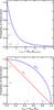 |
Fig. 5 Top panel: probability for the ratio of the magnetic field measurement of the plane-of-sky component and of the los component to yield a value of at least rmin. Bottom panel: probability for a magnetic field measurement of the plane-of-sky component (blue curve) and of the los component (red curve) to yield a fraction of at least fmin of the total magnetic flux density. |
Here we are concerned with the absolute values of the projected fields. In this situation, we can ignore the sign of ϑ and we can limit the analysis to half of the sphere. We encode the probability distribution of ϑ via the weighting function W(ϑ) = 2πcos(ϑ). The probability that projections with ϑ are less than or equal to some angle ϑp, 0 ≤ ϑ ≤ ϑp, is then 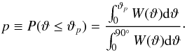 (5)Evaluation yields
 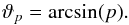 (6)We can use this result to evaluate the probability that projection effects lead to a specific ratio between the projected field strengths, r = Blos/Bpos. Substitution of Eq. (5) gives r = tan(ϑ). Here we choose to display the probability that the actual field strength ratio r is larger than some minimum value rmin, P(r>rmin). This essentially means that we use rmin = tan(ϑp) to calculate the limiting angle ϑp = arctan(rmin) that is then used to obtain P(r>rmin) as P(ϑ ≥ ϑp), i.e., the probability of having projection angles larger than ϑp. By definition, P(ϑ ≥ ϑp) = 1−P(ϑ ≤ ϑp) = 1−p, where we substituted Eq. (5). We then use p = sin(ϑp) as a consequence of Eq. (6) to eventually obtain P(r>rmin) = 1−sin(arctan [rmin]).
For completeness, we extend this formalism also to estimate the likelihood that a certain fraction of the magnetic field is projected into the plane of the sky, respectively, along the los. This aspect has already been discussed in detail by Heiles & Crutcher (2005). Assuming we wish to evaluate the probability that at least a fraction fmin = Bpos/B of the magnetic field is projected into the plane of the sky. Equation (5) gives the angle ϑ = arccos(fmin) that must not be exceeded to obtain the required projected field strength. Equation (5) describes the probability that this angle is not exceeded. Substitution then gives the probability that Bpos exceeds a certain fraction of the total field, Ppos = sin(arccos [fmin]). Now assume we wish to determine the probability that at least a fraction fmin = Blos/B of the magnetic field is projected along the los. Now Eq. (5) gives the angle ϑ = arcsin(fmin) that must not fall short of to obtain the required value of Blos. Thus, we need to know P(ϑ ≥ ϑp), which is by definition equal to 1−P(ϑ ≤ ϑp). Substitution yields Plos = 1−sin(arcsin [fmin] ) = 1−fmin as the probability that Blos exceeds a fraction fmin of the total field.
The probabilities Ppos(fmin) and Plos(fmin) are shown in Fig. 5. Note that Ppos always exceeds Plos by a significant factor. In particular, in a given situation it is always likely that Bpos represents a significant fraction of the total field strength. For example, we see that in 90% of all cases Bpos is at least 44% or more of the true field strength B. Blos, however, is more likely to be significantly smaller than B; only in 50% of all situations is Blos at least 50% of B. This discrepancy between the los and plane-of-sky projections is also seen in the mean projected field strengths. One finds 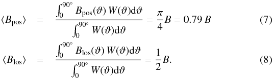 In general, plane-of-sky projections are much closer to the true field strength than los projections.
We note that Eq. (8) for Blos is consistent with that derived by Heiles & Troland (2005), who showed that statistically the average value of Blos is only half of the total field strength B. However, Eq. (7) shows that the same correction factor cannot be applied for Bpos (see also Heiles & Crutcher 2005). Our result might explain the studies that so far have found systematically higher field strengths based on Chandrasekhar-Fermi method relative to Zeeman measurements (e.g., Vallée & Fiege 2006, 2007a,b; Crutcher 2012).
5.2. Estimated vs. observed fields
We are in the convenient situation that we obtained two perpendicular components of the magnetic fields, i.e., the plane-of-sky and los components. These independent observations can be used to execute plausibility checks of these observations. First, we study the ratio between Blos and Bpos. This builds on the formalism derived in Sect. 5.1. We then compare the los component of the field to that obtained under the assumption that the cloud core is balanced against self-gravity.
5.2.1. Ratio between magnetic field components
The formalism in Sect. 5.1 permits us to estimate how likely certain ratios between field components are. Consider that we obtain a plane-of-sky magnetic field strength Bpos= 742 μG and a los component of Blos= 687 μG. The ratio r = Blos/Bpos discussed above is thus ~0.9. From Fig. 5 (top), we find that the probability of detecting the orthogonal components of at least this value, r ≥ 0.9, is 33%. This is a very reasonable result.
We thus conclude that observations finding Blos ≈ Bpos, as obtained in our case, are reasonable results. Values of r very different from unity would be unlikely to result from mere projection effects. In those situations, it would be more likely that observational artifacts drive the estimated field strengths.
We remark that dense cores with very high observed values of plane-of-sky magnetic fields are not ideal candidates for Zeeman detection experiments. As evident from Fig. 5 (top), only in 29% of all cases does one expect that Blos exceeds Bpos. Zeeman observations should be setup to be sensitive enough to detect fields as faint as 0.58·Bpos to be able to detect Zeeman signals with a probability ≥50%.
5.2.2. Fields assuming balance against self–gravity
We can also estimate the total magnetic field strength in the clump by following a virial analysis. For the clump properties tabulated in Table 3, we first gauge the turbulent support for the cloud. Section 4.2.1 shows that the CN emission traces the dense gas and that it is optically thin. Therefore, we use the CN velocity dispersion associated with the LSR velocity to measure the kinetic energy. We note that σv = 0.93 km s-1 is the sum of the thermal H2 and the non–thermal motions of the bulk gas (see Table 3). Then we follow Eq. (1b) in Kauffmann et al. (2013) and find the virial ratio α for turbulent support to be α = 0.2. As discussed in detail in Kauffmann et al., this is significantly lower than the critical value of ~2 for stability. This suggests that the clump is likely to be highly magnetized if stable. An ordered field perpendicular to the main axis is strongly in favor of this scenario. We use Eq. (16) of Kauffmann et al. to estimate the field strength for a magnetized clump,  (9)Following the definitions in Kauffmann et al., MΦ is the magnetic flux mass and MBE is the Bonner-Ebert mass. Thus, we derive a total field strength of 1640 μG.
Based on the results mentioned earlier, we infer that the los magnetic field is 687 μG, while the plane-of-sky field shows a very ordered structure perpendicular to the principal filament axis with an implied field strength of ~740 μG. Do the two complementary field estimates contradict each other? The expected los component based on virial analysis is given by Blos/ μG = [16402−7422] 1/2 = 1462. This is in contradiction with our Zeeman measurement of −687 ± 420 μG at a 1.8σ level.
Based on the probability distribution of orthogonal projections, we argued that the lack of a Zeeman signal is not a surprising result. However, there are a few other reasons to question the robustness of field determination using the methods above. First, the CF method uses the dispersion in the polarization angle. The observed polarization angle is an average over several turbulent cells along the los. The larger the number of cells, the smoother the field and smaller the dispersion in field angles. For our calculations, we assume a correction factor of 2 thatis consistent with sub-Alfvénic simulations, while super-Alfvénic models suggest a larger correction. However, super Alfvénic turbulence would manifest itself as a chaotic and complex field structure at odds with the observed smooth field structure. Nevertheless, a correction factor of 3 or higher would imply an even higher inconsistency with the Zeeman upper limit at >4σ level. This rather suggests that field strengths derived from polarization observations of this highly magnetized filament is not an overestimate. Second, systematic gas kinematics unrelated to turbulence can align the field making it more ordered. No such large scale field structure is evident in the polarization map toward G35.20w.
As far as Zeeman measurements are concerned, first, there could be a mutual cancellation of the Zeeman components within our 23.5′′ beam or exactly along our los owing to field reversals. If the latter is true, then even more sensitive observations like those with ALMA will fail to detect any signal. Simulations by Bertram et al. (2012) show that even for sub-Alfvénic turbulence, unfortunate angles between the los and the mean field direction can cause significant field reversals. Second, depletion of CN at the very center could weaken the detection considerably (Tassis et al. 2012). P11 report NH2D emission with high deuterium fractionation that is indicative of cold conditions conducive to depletion of heavy neutrals in G35.20w. However, similar to the results for low-mass prestellar cores (Hily-Blant et al. 2008), we also do not find a depletion hole in the CN integrated intensity map (see Fig. 2). However, we cannot rule out an abundance drop on smaller core scales.
5.3. Sub-Alfvénic and super-critical
Polarization measurements of a range of dense ISM structures, from pristine high-mass filaments (Pillai et al. 2015) to high-mass star-forming cores (Girart et al. 2009; Zhang et al. 2014; Li et al. 2015), have shown that magnetic fields play a dominant role from cloud to core scales.
A direct measurement of the implied strong field however, has been largely evasive. CN Zeeman observations in star-forming regions allow for the most direct determination of field strength in dense gas (Crutcher et al. 1996). Robust CN Zeeman observations to date have been made toward active high-mass star-forming regions as opposed to younger evolutionary phases. We compared our Zeeman measurements with a recent compilation of B-field estimates in more evolved high-mass regions (Falgarone et al. 2008). Using Blos as an approximation to the total field, Falgarone et al. find that protostellar clumps are critical to moderately super-critical. The threshold value is defined based on the mass-to-flux ratio M/ ΦB, where the magnetic flux ΦB = π ⟨ B ⟩ R2 is derived from the mean magnetic field and the radius of the cloud cross-section perpendicular to the magnetic field. The critical mass-to-flux ratio is (Nakano & Nakamura 1978) (M/ ΦB)cr = 1/(2πG1/2), where G is the gravitational constant. We calculate this ratio in terms of the observed column density and magnetic field following Eq. (7) of Pillai et al. (2015). We use ![Mathematical equation: \hbox{$B_{\rm{}tot}=[B_{\rm{}pos}^2+B_{\rm{}los}^2]^{1/2}=1011$}](/articles/aa/full_html/2016/07/aa27803-15/aa27803-15-eq199.png) μG as the total magnetic field. A clump is magnetically sub-critical if (M/ ΦB) < (M/ ΦB)cr. We derive a ratio of 1.5 (see Table 4), which is consistent with the mean mass-to-flux ratio derived by Falgarone et al. (2008) for star-forming clumps, but lower than the value derived by (Pillai et al. 2015) for pristine high-mass regions. This is expected because magnetized support in the early stages gives way to initial collapse as the clump evolves. Once accretion onto protostars is initiated, gravity overwhelms magnetic support, changing the field from sub-critical to super-critical.
μG as the total magnetic field. A clump is magnetically sub-critical if (M/ ΦB) < (M/ ΦB)cr. We derive a ratio of 1.5 (see Table 4), which is consistent with the mean mass-to-flux ratio derived by Falgarone et al. (2008) for star-forming clumps, but lower than the value derived by (Pillai et al. 2015) for pristine high-mass regions. This is expected because magnetized support in the early stages gives way to initial collapse as the clump evolves. Once accretion onto protostars is initiated, gravity overwhelms magnetic support, changing the field from sub-critical to super-critical.
What about turbulence? The Alfvén mach number is given by  , where vA = Btot/
 is the Alfvén speed. We find that even though turbulence is supersonic in the clump, ℳA = 0.4 and, thus, sub-Alfvénic. This is similar to the results for the starless high-mass regions in Pillai et al. (2015), while Falgarone et al. (2008) find their more evolved cores to be in the Alfvénic to super-Alfvénic domain. Localized feedback associated with star formation especially in the active accretion and ejection phase can lead to enhanced turbulence and, therefore, modify the dynamics from magnetic field dominated to an equipartition state. This evolution manifests in the form of ordered field structure in the early stages that are increasingly perturbed by enhanced turbulence and gravity to chaotic field orientations.
6. Summary
G35.20w is a young high-mass clump in W48 that appears to be undergoing collapse unless supported by a very strong field of 1640 μG (Sect. 4.1). Our CN N = 1−0 Zeeman effect measurement toward G35.20w yields a los field strength of −687 ± 420 μG (Sect. 4.2.2). Thermal dust continuum polarization indicates that the magnetic field direction is aligned with the minor axis of the clump. The dispersion in polarization angles also provides a plane-of-sky component of the magnetic field of ~740 μG (Sect. 4.3). We show that plane-of-sky projections are much closer to the true field strengths than los projections (Fig. 5). The mass-to-flux ratio exceeds its critical value by a factor 1.5, indicating considerable magnetic support. Forces induced by the magnetic field significantly exceed those owing to the turbulent support (ℳA = 0.4).
Acknowledgments
We thank the IRAM 30 m staff for hosting us. We thank Kazi Rygl for providing us Herschel based mass and temperature maps. T.P. acknowledges support from the Deutsche Forschungsgemeinschaft, DFG via the SPP (priority program) 1573 “Physics of the ISM”. T.P. and J.K. thank Nissim Kanekar for an invitation to the National Centre for Radio Astrophysics (NCRA) in Pune, India where some parts of this project were completed. We thank the anonymous referee for pointing out the reference to the work by Heiles & Crutcher (2005) during the revision of this manuscript.
References
- Bertram, E., Federrath, C., Banerjee, R., & Klessen, R. S. 2012, MNRAS, 420, 3163 [NASA ADS] [Google Scholar]
- Chandrasekhar, S., & Fermi, E. 1953, ApJ, 118, 116 [NASA ADS] [CrossRef] [MathSciNet] [Google Scholar]
- Crutcher, R. M. 1999, ApJ, 520, 706 [NASA ADS] [CrossRef] [Google Scholar]
- Crutcher, R. M. 2012, ARA&A, 50, 29 [NASA ADS] [CrossRef] [Google Scholar]
- Crutcher, R. M., Troland, T. H., Lazareff, B., & Kazes, I. 1996, ApJ, 456, 217 [NASA ADS] [CrossRef] [Google Scholar]
- Curran, R. L., Chrysostomou, A., Collett, J. L., Jenness, T., & Aitken, D. K. 2004, A&A, 421, 195 [NASA ADS] [CrossRef] [EDP Sciences] [Google Scholar]
- Falceta-Gonçalves, D., Lazarian, A., & Kowal, G. 2008, ApJ, 679, 537 [NASA ADS] [CrossRef] [Google Scholar]
- Falgarone, E., Troland, T. H., Crutcher, R. M., & Paubert, G. 2008, A&A, 487, 247 [NASA ADS] [CrossRef] [EDP Sciences] [Google Scholar]
- Girart, J. M., Beltrán, M. T., Zhang, Q., Rao, R., & Estalella, R. 2009, Science, 324, 1408 [NASA ADS] [CrossRef] [PubMed] [Google Scholar]
- Hakobian, N. S., & Crutcher, R. M. 2011, ApJ, 733, 6 [NASA ADS] [CrossRef] [Google Scholar]
- Heiles, C., & Crutcher, R. 2005, in Cosmic Magnetic Fields, eds. R. Wielebinski, & R. Beck (Berlin: Springer Verlag), Lect. Notes Phys., 664, 137 [Google Scholar]
- Heiles, C., & Troland, T. H. 2005, ApJ, 624, 773 [NASA ADS] [CrossRef] [Google Scholar]
- Heitsch, F., Zweibel, E. G., Mac Low, M.-M., Li, P., & Norman, M. L. 2001, ApJ, 561, 800 [NASA ADS] [CrossRef] [Google Scholar]
- Hildebrand, R. H., Kirby, L., Dotson, J. L., Houde, M., & Vaillancourt, J. E. 2009, ApJ, 696, 567 [NASA ADS] [CrossRef] [Google Scholar]
- Hily-Blant, P., Walmsley, M., Pineau Des Forêts, G., & Flower, D. 2008, A&A, 480, L5 [NASA ADS] [CrossRef] [EDP Sciences] [Google Scholar]
- Houde, M., Vaillancourt, J. E., Hildebrand, R. H., Chitsazzadeh, S., & Kirby, L. 2009, ApJ, 706, 1504 [NASA ADS] [CrossRef] [Google Scholar]
- Kauffmann, J., & Pillai, T. 2010, ApJ, 723, L7 [NASA ADS] [CrossRef] [Google Scholar]
- Kauffmann, J., Bertoldi, F., Bourke, T. L., Evans, II, N. J., & Lee, C. W. 2008, A&A, 487, 993 [NASA ADS] [CrossRef] [EDP Sciences] [Google Scholar]
- Kauffmann, J., Pillai, T., Shetty, R., Myers, P. C., & Goodman, A. A. 2010, ApJ, 712, 1137 [NASA ADS] [CrossRef] [Google Scholar]
- Kauffmann, J., Pillai, T., & Goldsmith, P. F. 2013, ApJ, 779, 185 [NASA ADS] [CrossRef] [Google Scholar]
- Li, H.-B., Goodman, A., Sridharan, T. K., et al. 2014, Protostars and Planets VI, 101 [Google Scholar]
- Li, H.-B., Yuen, K. H., Otto, F., et al. 2015, Nature, 520, 518 [CrossRef] [Google Scholar]
- Matthews, B. C., McPhee, C. A., Fissel, L. M., & Curran, R. L. 2009, ApJS, 182, 143 [NASA ADS] [CrossRef] [Google Scholar]
- Maury, A. J., Wiesemeyer, H., & Thum, C. 2012, A&A, 544, A69 [NASA ADS] [CrossRef] [EDP Sciences] [Google Scholar]
- McKee, C. F., & Tan, J. C. 2002, Nature, 416, 59 [NASA ADS] [CrossRef] [PubMed] [Google Scholar]
- Nakano, T., & Nakamura, T. 1978, PASJ, 30, 671 [NASA ADS] [Google Scholar]
- Ossenkopf, V., & Henning, T. 1994, A&A, 291, 943 [NASA ADS] [Google Scholar]
- Ostriker, E. C., Stone, J. M., & Gammie, C. F. 2001, ApJ, 546, 980 [NASA ADS] [CrossRef] [Google Scholar]
- Pillai, T., Kauffmann, J., Wyrowski, F., et al. 2011, A&A, 530, A118 [NASA ADS] [CrossRef] [EDP Sciences] [Google Scholar]
- Pillai, T., Kauffmann, J., Tan, J. C., et al. 2015, ApJ, 799, 74 [NASA ADS] [CrossRef] [Google Scholar]
- Rygl, K. L. J., Goedhart, S., Polychroni, D., et al. 2014, MNRAS, 440, 427 [NASA ADS] [CrossRef] [Google Scholar]
- Tan, J. C., Kong, S., Butler, M. J., Caselli, P., & Fontani, F. 2013, ApJ, 779, 96 [NASA ADS] [CrossRef] [Google Scholar]
- Tan, J. C., Beltrán, M. T., Caselli, P., et al. 2014, Protostars and Planets VI, 149 [Google Scholar]
- Tassis, K., Willacy, K., Yorke, H. W., & Turner, N. J. 2012, ApJ, 754, 6 [NASA ADS] [CrossRef] [Google Scholar]
- Thompson, M. A., Gibb, A. G., Hatchell, J. H., Wyrowski, F., & Pillai, T. 2005, in The Dusty and Molecular Universe: A Prelude to Herschel and ALMA, 425 [Google Scholar]
- Thum, C., Wiesemeyer, H., Paubert, G., Navarro, S., & Morris, D. 2008, PASP, 120, 777 [NASA ADS] [CrossRef] [Google Scholar]
- Vallée, J. P., & Fiege, J. D. 2006, ApJ, 636, 332 [NASA ADS] [CrossRef] [Google Scholar]
- Vallée, J. P., & Fiege, J. D. 2007a, AJ, 133, 1012 [NASA ADS] [CrossRef] [Google Scholar]
- Vallée, J. P., & Fiege, J. D. 2007b, AJ, 134, 628 [NASA ADS] [CrossRef] [Google Scholar]
- Zhang, B., Zheng, X. W., Reid, M. J., et al. 2009, ApJ, 693, 419 [NASA ADS] [CrossRef] [Google Scholar]
- Zhang, Q., Qiu, K., Girart, J. M., et al. 2014, ApJ, 792, 116 [NASA ADS] [CrossRef] [Google Scholar]
- Zinnecker, H., & Yorke, H. W. 2007, ARA&A, 45, 481 [NASA ADS] [CrossRef] [Google Scholar]
All Tables
All Figures
|
Fig. 1 G35.20w SCUBA archival 850 μm polarization vectors rotated by 90° to show the magnetic field orientation, overlaid on SCUBA 850 μm dust continuum archival data (color scale). The position offsets are w.r.t. the coordinates given in Table 1. The box shows the region around our IRAM 30 m CN observations to which we confine our analysis. Polarization data is only shown where the polarization level is ≥3σ, corresponding to an uncertainty in position angle ≤9.5°. The length of the Bpos vector represents the percentage of polarization. |
| In the text | |
|
Fig. 2 CN(N = 1 → 0,J = 1/2 → 1/2) (left) and J = 1/2 → 3/2 (right) spectrum toward G35.20w. The LSR velocity is shown with respect to the component at 113 499.64 MHz (red dashed line). |
| In the text | |
|
Fig. 3 Left: SCUBA 850 μm dust continuum archival data (colorscale) and CN intensity integrated over the 113 170.49 MHz hyperfine from 34 to 42 km s-1 (contours, 1.2 to 4 in steps of 0.3 K km s-1). The offsets positions for the CN map and the IRAM 30 m beam are shown as black squares and dashed circle respectively. Right: correlation plot of 850 μm flux (smoothed to 23.5′′) and CN integrated intensity. |
| In the text | |
|
Fig. 4 Weighted average of all Zeeman-sensitive transitions (black spectrum) after smoothing to 0.4 km s-1 velocity resolution, and best-fitting Zeeman signal (red spectrum). The green highlighting roughly indicates the spectral channels that we considered in the fitting process. |
| In the text | |
|
Fig. 5 Top panel: probability for the ratio of the magnetic field measurement of the plane-of-sky component and of the los component to yield a value of at least rmin. Bottom panel: probability for a magnetic field measurement of the plane-of-sky component (blue curve) and of the los component (red curve) to yield a fraction of at least fmin of the total magnetic flux density. |
| In the text | |
Current usage metrics show cumulative count of Article Views (full-text article views including HTML views, PDF and ePub downloads, according to the available data) and Abstracts Views on Vision4Press platform.
Data correspond to usage on the plateform after 2015. The current usage metrics is available 48-96 hours after online publication and is updated daily on week days.
Initial download of the metrics may take a while.