| Issue |
A&A
Volume 591, July 2016
|
|
|---|---|---|
| Article Number | A36 | |
| Number of page(s) | 6 | |
| Section | Astrophysical processes | |
| DOI | https://doi.org/10.1051/0004-6361/201527711 | |
| Published online | 07 June 2016 | |
Impact of inclination on quasi-periodic oscillations from spiral structures
1
AstroParticule & Cosmologie (APC), UMR 7164, Université Paris
Diderot,
10 rue Alice Domon et Leonie Duquet,
75205
Paris Cedex 13,
France
e-mail:
varniere@apc.univ-paris7.fr
2
Observatoire de Paris/LESIA, 5 place Jules Janssen, 92195
Meudon Cedex,
France
3
Nicolaus Copernicus Astronomical Center, ul. Bartycka
18, 00-716
Warszawa,
Poland
Received: 6 November 2015
Accepted: 18 March 2016
Context. Quasi-periodic oscillations (QPOs) are a common feature of the power spectrum of X-ray binaries. Currently it is not possible to unambiguously differentiate the large number of proposed models to explain these phenomena through existing observations.
Aims. We investigate the observable predictions of a simple model that generates flux modulation: a spiral instability rotating in a thin accretion disk. This model is motivated by the accretion ejection instability (AEI) model for low-frequency QPOs (LFQPOs). We are particularly interested in the inclination dependence of the observables that are associated with this model.
Methods. We develop a simple analytical model of an accretion disk, which features a spiral instability. The disk is assumed to emit blackbody radiation, which is ray-traced to a distant observer. We compute pulse profiles and power spectra as observed from infinity.
Results. We show that the amplitude of the modulation associated with the spiral rotation is a strong function of inclination and frequency. The pulse profile is quasi-sinusoidal only at low inclination (face-on source). As a consequence, a higher-inclination geometry leads to a stronger and more diverse harmonic signature in the power spectrum.
Conclusions. We present how the amplitude depends on the inclination when the flux modulation comes from a spiral in the disk. We also include new observables that could potentially differentiate between models, such as the pulse profile and the harmonic content of the power spectra of high-inclination sources that exhibit LFQPOs. These might be important observables to explore with existing and new instruments.
Key words: X-rays: binaries / accretion, accretion disks / instabilities
© ESO, 2016
1. Introduction
Quasi-periodic oscillations (QPOs) are a common feature of the power spectrum of black-hole X-ray binaries (see e.g., the reviews by Remillard & McClintock 2006; Done et al. 2007, and references therein). Early on, QPOs were observed outside of the X-ray band, for example in the optical (Motch et al. 1983) and recently in the infrared (Kalamkar et al. 2015). They are characterized by a Lorentzian component in the power spectrum of the source, distinguished from broader noisy peaks by a condition on the coherence parameter (Q = νLF/FWHM ≳ 2, with many cases at Q> 10). Depending on their frequencies they are either called a high-frequency QPO (~40 to 500 Hz) or low-frequency QPO for frequencies within approximately [0.1−30] Hz. Low-frequency QPOs (LFQPOs) are seen when the power-law component of the spectrum is strong (such as the hard, hard/intermediate states). This suggests that these oscillations are not only linked to the thermal disk but also to a nonthermal component which could be either a hot inner flow (Done et al. 2007) or some kind of a hot corona above the disk. Different types of LFQPOs have been introduced based mainly on their characteristics. In this article we are focusing on the most frequent one, namely the type-C LFQPO, which has the interesting property of having a strongly varying frequency νLF that seems to be correlated with the disk flux. This may be a hint that LFQPOs have an origin in the disk while also being reprocessed in a corona or hot inner flow.
While we have a lot of observations, no consensus on the origin of the modulation has yet been achieved. There are several classes of models, depending on what causes the modulation. Among all the families of models, one originated from Stella & Vietri (1998) which advocated that the Lense-Thirring precession of particles around a rotating black hole could produce LFQPOs. This family was further extended by Schnittman et al. (2006) and more recently Ingram et al. (2009) and Nixon & Salvesen (2014). Another family is based on different kinds of instabilities occuring in either the disk or the corona. Among those Tagger & Pellat (1999) looked at a spiral instability driven by magnetic stresses (the accretion-ejection instability, AEI). Chakrabarti & Manickam (2000) propose that QPOs are due to radiation emitted by oscillating shocks in the disk while Titarchuk & Fiorito (2004) consider a transition layer that comptonizes the outer disk. In yet another approach, Cabanac et al. (2010) consider a magneto-acoustic wave propagating in the corona while O’Neill et al. (2011) present magnetohydrodynamic (MHD) simulations of blackhole accretion flow exhibiting a dynamo cycle with a characteristic time that coincides with LFQPOs. While several models have links with emission outside the X-ray band, for example in the case of the AEI (Varnière & Tagger 2002), the most developed model at the moment is the one by Veledina et al. (2013, 2015), which explains this multiwavelength phenomena by elaborating on the precessing hot flow model of Ingram et al. (2009). It is worth noting that their curve of rms as a function of the inclination of the system is quite different from the one presented here, and observation might be able to distinguish between them.
Despite the amount of ongoing modeling, up to now QPO models have focused mainly on explaining the frequency observed in the power spectrum (PDS). While this is essential, it is only the first observable we had access too and all of the models fulfilled this requirement since they were created to answer it. It is therefore interesting to look for other observables that might help to differentiate between models. Some of those we already have access to through observation, such as the amplitude, but also some we do not have yet complete access to, such as the pulse profile.
In this article we are interested in revisiting the AEI model and expand on a previous Newtonian approach (Varnière & Blackman2005) to include a wider range of frequencies and general-relativistic effects. In particular, we want to see how the observables are affected by the general relativistic effects in higher-inclination systems. Already with this simple model, we aim at studying the evolution of the amplitude of the spiral modulation as a function of the QPO frequency and to do this for high- and low-inclination systems. We are also interested in how this affects the shape of the pulse profile and hence the harmonic content of its power spectrum. Section 3 presents our simple model of a disk featuring a spiral instability. Section 4 shows the evolution of the amplitude with inclination and QPO frequency. Section 5 analyzes the pulse profile for various inclinations and discusses the corresponding power spectra.
2. The accretion-ejection instability as a model for LFQPO
In a nutshell, the AEI is a global spiral instability which occurs in the inner region of a fully magnetized (close to equipartition) accretion disk (Tagger & Pellat 1999). The energy is extracted from the disk (hence allowing accretion) through the spiral wave and then stored in a Rossby vortex, which is located at the corotation radius of the spiral (the point where the spiral and accretion disk rotate at the same velocity), which is typically a few times the inner radius of the disk. In the presence of a low-density corona, the Rossby vortex will twist the footpoint of the magnetic field line. This causes an Alfven wave to be emitted toward the corona, therefore linking accretion and ejection (Varnière & Tagger 2002) which, in turn, has the unique consequence of linking what is happening in the thermal disk with what is happening at higher energy in the corona. This way the modulation in the disk will be transmitted to the corona.
Here we will summarize salient points and observational tests of the AEI as the origin of the LFQPO. We focus on the X-ray data which represent the bulk of the observations:
-
The rotation frequency of the spiral is the orbital frequency at the corotation radius, rc , which is predicted to be a few tenths of the orbital frequency at the inner edge of the disk. This frequency is consistent with the LFQPO frequency ( Tagger & Pellat 1999).
-
As the position of the inner edge of the disk evolves during the outburst, the rotation frequency of the spiral also changes, which can be directly compared with observation (Varnière et al. 2002).
-
By including general relativity through the existence of a last stable orbit and orbital velocity profile, the AEI explains the observed turnover in the correlation between the color radius (=Inner disk radius, as determined by the spectral fits) and the LFQPO frequency (Rodriguez et al. 2002; Mikles et al. 2009).
-
In the Newtonian approximation, the AEI is able to create a thermal flux modulation (Varnière & Blackman 2005) in the range of the observed one.
-
Once the AEI is established, 2D MHD simulations show a nearly steady rotation pattern, and is thus able to account for persistent LFQPOs.
-
The AEI transfers energy and angular momentum toward the corona by Alfven waves, thus providing a supply of Poynting flux that may produce the compact jet often observed in the low-hard state (Varnière & Tagger 2002) .
Because of these characteristics, the model based on the assimilation of the AEI with the origin of the LFQPO has since been expanded, first as a scenario for the β class of GRS 1915+105 (Tagger et al. 2004), then as a way of classifying blackhole states (Varniere et al. 2011) and, more recently, a possible explanation for the different types of LFQPO (Varniere et al. 2012).
3. Amplitude of the modulation for a spiral model
Rather than looking at the formation of the spiral instability in a disk, we decided to focus on its consequence on the emission. Consequently, rather than taking full MHD simulations of the AEI in the different conditions we wish to explore, we decided to create a simple, analytical model that mimics the temperature profile of the AEI to test the different parameters more cleanly. Indeed, in a full fluid simulation, changing one parameter in the initial condition can have repercussions on several observable parameters and, therefore, it is harder to study the different effects separately. We consider a geometrically thin accretion disk, introduce a spiral feature in this disk at a higher temperature, and consider the emission of blackbody radiation. Also, through the AEI, energy and angular momentum is sent toward the corona (Varnière & Tagger 2002), but the exact amount depends on many parameters that are not easily constrained by observation. Here we take a simpler approach; rather than adding multiple unconstrained parameters, we decide to stick to a very simple, analytic model of the thermal emission in the disk for which we have more constraints. This means that we are able to predict the light curve of LFQPOs in the lower energy part of the spectrum (1 keV), leaving a more in-depth study of the LFQPO rms-spectrum as a function of energy for a more complex, simulation-based, model.
We have therefore taken a simple, analytic model of a disk that features a spiral structure, which is able to reproduce the main aspects of the AEI model as seen in simulations (see for example Varniere et al. 2012), and see how the flux is thus modulated.
3.1. Parametrization of the disk temperature profile
We consider a geometrically thin disk surrounding a Schwarzschild blackhole of mass M. The disk extends from a varying inner radius rin to a fixed outer radius rout = 500 M. To keep a simple structure, we choose to have the temperature profile T0(r) ∝ r− η. In agreement with the thin disk blackbody model, we took η = 0.75 as the equilibrium temperature profile. This profile is then fixed by choosing the temperature at the innermost stable circular orbit (ISCO), labeled TISCO.
This equilibrium disk is assumed to give rise to a spiral instability. We model this phenomena in a very simple way, just describing the hotter spiral structure rotating in the equilibrium disk, in agreement with numerical simulations of the AEI (see for example Varniere et al. 2012). The temperature of the disk with this added spiral feature reads ![\begin{eqnarray} \label{eq:T} T(t,r,\varphi) &=& T_0(r) \\ \nonumber &&\times\left[1 + \gamma \left(\frac{r_{\rm c}}{r}\right)^\beta\mathrm{exp}\left(-\frac{1}{2}\left(\frac{r-r_{\rm s}(t,\varphi)}{\delta \,r_{\rm c}}\right)^2\right)\right]^2 , \\ \nonumber \end{eqnarray}](/articles/aa/full_html/2016/07/aa27711-15/aa27711-15-eq17.png) (1)where the perturbation term between brackets describes the spiral pattern. The parameter γ encodes the temperature contrast between the spiral and the surrounding disk. The quantity rc is the corotation radius of the spiral. The spiral temperature is thus following a power-law decrease when moving away from r = rc, with an exponent β. This ensures that the spiral will fade away into the disk after a few turns. In the latter Gaussian term, rs is a shape function encoding the spiral feature. It ensures that the spiral’s width is a factor δ times the corotation radius. The shape function reads
(1)where the perturbation term between brackets describes the spiral pattern. The parameter γ encodes the temperature contrast between the spiral and the surrounding disk. The quantity rc is the corotation radius of the spiral. The spiral temperature is thus following a power-law decrease when moving away from r = rc, with an exponent β. This ensures that the spiral will fade away into the disk after a few turns. In the latter Gaussian term, rs is a shape function encoding the spiral feature. It ensures that the spiral’s width is a factor δ times the corotation radius. The shape function reads  (2)where α is the spiral opening angle and Ω(rc) is the Keplerian frequency at rc. Ultimately it is the rotation frequency of the spiral and the frequency at which the flux is modulated.
3.2. Model parameters
The spiral parameters are chosen to (1) be in agreement with numerical simulations of the AEI and (2) produce reasonable values of amplitude. The present study is not devoted to the detail of the dependency of observables on the model parameters (see Varnière & Blackman 2005, for a parameter study in the Newtonian approximation). Instead, we fix the parameters that represent the spiral and then study, in a frozen framework, how the inclination impacts the amplification, and this for a sample of modulation frequencies representative of the type-C LFQPO.
In this respect, the temperature at the ISCO is taken to be TISCO = 107 K, thus emitting blackbody radiation mainly around 1 keV and the disk is geometrically thin with an aspect ratio of H/r = 0.01. The power-law exponent encoding the temperature decrease away from r = rc is set to β = 0.5. This ensures that the spiral will be negligible within a few turns. The opening angle is chosen to be α = 0.1, in agreement with numerical simulations (Varniere et al. 2011, 2012). Then we decided to use and freeze the parameters of the spiral so that a QPO of about 10 Hz had an amplitude of about 10% at an inclination of 70°. This gives γ = 2.2 and δ = 0.2, which are conservative compared to the maximum reached in numerical simulations (Varniere et al. 2012). These same parameters gave an amplitude of about 3% at an inclination of 20°.
In the rest of the paper, only the inclination at which the system is observed and the position of the inner edge of the disk will be varied. This produces a large set of QPO frequencies. Indeed, as shown by Tagger & Pellat (1999), the corotation radius of the spiral is a few times the inner radius of the disk. Here we chose to keep rc/rin fixed at a typical value of 2, so that, as the inner radius varies, so the corotation radius. We consider an inner edge of the disk varying in the range[1.5 rISCO,15 rISCO] which creates modulation frequencies in the range [1 Hz,42 Hz] for M = 10 M⊙.We do not compute very-low-frequency QPOs (below 1 Hz) because, in our model, they demand both a very large disk (the corotation radius for this kind of frequency is far from the last stable orbit) and a very fine grid resolution, which translates into overly long computing time. We also consider one simulation at 42 Hz, thus above the maximum observed LFQPO frequency, to capture the tendency of the rms amplitude towards the highest frequency LFQPOs.
3.3. Emission from the disk and ray-tracing
The whole disk is assumed to simply emit as a blackbody at the temperature T(t,r,ϕ). So the specific intensity emitted at some position in the disk is  (3)where the superscript em refers to the emitter’s frame, i.e., a frame corotating (at the local Keplerian frequency) with the disk. This emitted intensity is then transformed to the distant observer’s frame using the constancy along geodesics of Iν/ν3. Thus
  (4)where g = νobs/νem is the redshift factor. This redshift factor is, in particular, responsible for the so-called beaming effect, which makes the observed specific intensity stronger when the emitter travels towards the observer and fainter in the opposite case. In the following we use hνobs = 1 keV.
To compute maps of specific intensity  , we use the open-source general relativistic ray-tracing code GYOTO (Vincent et al. 2011) into which we added the parametrized disk profile that was defined in the previous section. Null geodesics are integrated in the Schwarzschild metric, backwards in time from a distant observer at some inclination with respect to the disk. Inclination is equal to the angle between the observer’s line of sight and the normal to the black hole’s equatorial plane. From such maps of specific intensity, the light curve (flux as a function of time) is derived by summing all pixels weighted by the element of solid angle, which is subtended by each pixel.
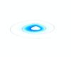 |
Fig. 1 Logscale view of the inner region of an accretion disk, having a hotter m = 1 spiral wave with a corotation radius of rc = 10 rISCO, seen at an inclination of i = 70°. |
Figure 1 shows, in logscale, a spiral with a corotation radius located at rc = 10 rISCO. It shows the spiral arm fading into the background disk following the power-law decrease of the amplitude as the spiral expands. Before it reaches the end of the disk, the spiral has fully faded. Most of the emission actually comes from the first two turns of the spiral, close to r = rc, and we only consider the full spiral for consistency.
4. Impact of frequency and inclination on the amplitude
We can now take advantage of our analytical model and test how the amplitude of the modulation that comes from the rotating spiral behaves with respect to the position of the corotation radius, namely the frequency and the inclination of the system. While it seems easy to obtain observational data in the first case (amplitude versus νQPO), the second case (amplitude versus inclination of the system) seems less attainable. Here we need to clarify that, even this first case is not as easily compared to observation as it seems. Indeed, we are trying to look at the impact of one parameter at a time, therefore no temporal evolution is taken into account. We are not “monitoring” the evolution of the instability as the inner edge of the disk moves but, instead, looking at the same spiral in different locations, meaning all the other parameters are frozen while we take snapshots with different inner edges of the disk.
To be able to compare the different lightcurves on the same plot we renormalize them with the time being t/T where T is the period of each modulation, and the flux being f/fmean, where fmean is the mean flux of each particular curve. This allows for an easier comparison of the shape of each lightcurve independantly of its total flux and period. For all models, we define the amplitude as  (5)where fmin and fmax are the extremal values of flux.
4.1. Origin of the modulation
In the case of a spiral, or any nonaxisymetrical structure orbiting in the disk, one would get a modulation as a combination of two effects. First, as the spiral orbits around the disk, its observed intensity is modulated by the beaming effect: this will be stronger on the approaching side and fainter on the receding side. In addition, the projected emitting area on the observer’s sky varies with time as the spiral rotates, which also creates a flux modulation. From this, it appears that the most important parameter of the spiral, as far as amplitude is concerned, is its temperature contrast with the disk (encoded in the γ parameter). The higher the contrast with the disk, the greater the amplitude of the modulation.
In Fig. 2 we show the renormalized lightcurves for three positions of the inner edge (and consequently of the spiral’s corotation radius) for a disk seen under an inclination of 20° (close to face-on). Several facts already appear on this plot. While all of the spirals have the same amplitude, γ, the amplitude increases as the corotation radius is further away in the disk.
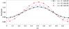 |
Fig. 2 Renormalized light curves obtained for the same spiral with three values of the inner edge of the disk and associated corotation radii. Here the system is viewed at an inclination i = 20° and the black dots represent rc = 4rISCO, blue triangles rc = 10rISCO and red squares rc = 20rISCO. |
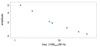 |
Fig. 3 Evolution of the amplitude of the modulation as function of the QPO frequency, meaning Ω(rc = 2 rin), for an inclination i = 20°. |
This can easily be understood as follows. Given the temperature profile in Eq. (1), it is straightforward to obtain that the ratio between the maximum temperature along the spiral (i.e., at the corotation radius r = rc) and the temperature at the inner edge is Tspi/Tin = (1 + γ)2/ 2 with γ = 2.2 in our case. It is then easy to compute the corresponding ratio of blackbody emission Bν(Tspi) /Bν(Tin) as a function of the value of the inner radius. This ratio is a strongly increasing function of the inner radius. As a consequence, the spiral dominates more and more the inner regions of the disk as the inner radius increases. Thus, at similar spiral parameters, the amplitude increases with a receding disk. It is important to note that this is valid for similar spiral parameters and that, for widely varying spiral parameters, the amplitude behavior with respect to the inner edge of the disk could be reversed. On the same note, if we relax the constraint on the corotation rc = 2rin1, we can see for the same rc and spiral parameters, the modulated part of the flux is constant while, changing the position of the inner edge of the disk changes the unmodulated part of the flux, hence impacting the total rms amplitude of the modulation.
Another interesting point is that, at low inclination, the modulation closely resembles a sine function. It takes a Fourier decomposition to see the presence of small amplitude harmonics and is often limited to the first few harmonics (more about this in Sect. 5). Those also become stronger similarly to the amplitude when the inner edge of the disk is further away from the ISCO.
4.2. Impact of QPO frequency on the amplitude
Following the observation from Fig. 2. that the same spiral has a stronger amplitude as it is further away in the disk, we can plot the evolution of the amplitude of the modulation created by the same-parameter spirals as a function of the couple (rin, rc = 2 rin). With the parameters we fixed, we get an approximate 3% amplitude at a frequency of 10 Hz for the low inclination (i = 20°) case.
As we can see in Fig. 3, we follow a wide range of frequencies and see a steady increase in the amplitude as the frequency gets lower. This is in part linked to the fact that we are keeping the inner egde of the disk and the corotation radius in a locked ratio of rc = 2rin. Indeed, as the frequency increases it means that the inner edge of the disk gets closer to the last stable orbit, hence gets hotter and emits more in the observation band. As a consequence the modulation amplitude over the total emission is lower.
Here we need to be cautious, since this plot is done for the same spiral parameters but looking at different frequencies, meaning that it does not represent an evolution of the spiral responsible for the modulation. In the case of a temporal evolution, such as the one would get in a full MHD simulation and/or a full outburst, the spiral would also change (e.g., its amplitude) hence it would influence the precise shape of this plot. Nevertheless, it shows a strong propensity of the amplitude to decrease with frequency.
4.3. Amplitude dependence on inclination
One parameter that can change a lot, both the beaming effect and the projected emitting surface (and thus, the modulation) is the inclination at which the system is observed. Using observation alone this is not something that can easily be studied. However, Motta et al. (2015) show one of the first statistical studies demonstrating that higher-inclination systems tend to have a higher amplitude for the QPO than is the case for lower-inclination systems. It is therefore interesting to determine how the amplitude in an almost edge-on system (inclination 70°) and an almost face-on system (inclination 20°) would compare for exactly the same spiral parameters. For this reason we focus on the ratio between amplitudes at different inclinations and not their actual value.
Figure 4 shows the evolution of the ratio of the amplitude at inclination 70° over the amplitude at inclination 20° as a function of the position of the structure in the disk, namely rc, which is related to the frequency through the mass of the central object. Indeed, as in observation, one cannot observe the same system at different inclinations, it seems easier to produce a plot that could be scaled to the different masses of the objects.
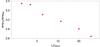 |
Fig. 4 Evolution of the ratio of the amplitude at inclination 70° over the amplitude at inclination 20° as a function of the position of the structure given in units of the ISCO radius. |
While high inclination system always have a higher amplitude than low inclination system for the same physical parameters, we see than the ratio is dependant on the frequency of the modulation, linked to the position of the co-rotation radius. We see that the ratio decreases from ~3.5 for small rc, which translates to a higher frequency, to ~2.5 for larger rc, meaning a lower frequency. Indeed, this is related to the fact that the flux modulation is, in particular, due to the beaming factor. The flux will be boosted when the hottest parts of the spiral are on the approaching side of the disk, while the flux will be deboosted when these hottest parts are on the receding side. This boosting is a strong function of inclination: it will be bigger for close to edge-on views because the emitter will then be traveling almost exactly towards the observer. Furthermore, as we get far from the blackhole, the effect of the beaming will decrease, and will thus be less important for lower QPO frequencies (higher rc).
Figure 4 is impossible to compare directly with the results of Motta et al. (2015) since these authors average several sources, hence different blackhole masses, which in turn mean the same QPO frequencies do not correspond to the same distance in the disk, and to different inclinations and different times of their outburst evolution. On the contrary, here we look at the amplitude dependence on inclination for exactly the same system at different QPO frequencies, which is clearly not what happens in an outburst, since the source evolves dynamically. Nevertheless, it is already interesting to see that the same system, under the same conditions, does indeed have a different amplitude, depending on the inclination of the system, and that this difference evolves, depending on the position of the spiral in the disk.
5. Case of the pulse profile in high-inclination systems
While the previous section focused on the amplitude of the QPO, there is more to QPOs than just a frequency and an amplitude. Indeed, here we have access to the exact pulse profile. This allows us to study the more direct impact of inclination on the lightcurve.
5.1. Shape of the pulse
In Fig. 5, we show one period of three pulse profiles for three different locations of the spiral, as seen from an inclination of 70°. We have chosen the same position/frequency as in Fig. 2 so that it is easier to compare both cases. The main difference with the 20° inclination case is that, at high inclination, the detailed shape of the pulse is clearly not sinusoidal. This implies that any Fourier decomposition will contain more than one frequency, even when the initial signal in our model only has one. This effect comes from Doppler boosting and the varying apparent area of the spiral on the observer’s sky, and it gets stronger with inclination. We explore how this should be visible on the PDS in the next section.
However, it is worth mentioning another possible way of detecting this change in the shape of the pulse profile, even without having access to its details. Indeed, in Fig. 5 we see that for high-inclination systems, the lightcurves are not symmetrical with respect to the mean values. While this is only a few % and hardly detectable all the time, we may find some high-inclination systems that have a strong QPO around a few Hz in a steady enough observation in which we can try to assess the time spent above and below the mean value. Perhaps this would be worth investigating in, for example, the Plateau state of GRS 1915+105? While the resolution needed to look at it on a pulse timescale is beyond the capacity of past and present satellites, it would be an interesting new observable to differentiate between models for future missions.
5.2. Impact on the PDS
As seen in the previous section, the shape of the pulse profile departs more and more from a sinusoid as the inclination of the system increases from almost face-on to almost edge-on. When looking at it in the Fourier space, this departure translates into more harmonics that might be more easily detectable than a difference in the pulse profile.
To compute the power density spectrum, we extended our lightcurve to 20 orbits and added a 1 /f noise. Also, as we are interested in comparing the extent of the harmonic structure with respect to inclination, we re-normalized the amplitude of the fundamental peak in each case to 1. This allows us to compare only the relative strength of the different peaks.
In the case of a QPO frequency of about 2.5 Hz (hence a corotation radius of 20 rISCO), we already have a first harmonic present even at the inclination of 20°, while the pulse profile looks sinusoidal (see Fig. 2.).In the case of a close to edge-on view, we get a much richer and stronger harmonic content. Indeed, we have not one, as in the close to face-on view, but several additional and stronger peaks, while the simulation we ran had one mode present (one-arm spiral). This behavior of richer harmonic content for high-inclination systems does not seem to depend on the frequency of the modulation, though it would be easier to detect for higher amplitude fundamentals, hence smaller frequencies.
However, care must be taken when interpreting this result since instabilities that give rise to spiral waves in a disk tend to have more than one mode and therefore the original signal could be more complex than the case with only one mode that is presented here. The different modes are in a close to harmonic relationship and could therefore lead to harmonic peaks in the PDS. Nevertheless, these instabilities also tend to have such a degree of competition between modes (more as a transition from one to another) and it should not be difficult to detect this.
6. Conclusion
In this paper we looked at a simplified version of the spiral formed by accretion ejection instability and studied the lightcurves that are observable from this type of system. Our main goal was to study how the amplitude of the observed lightcurve depends not only on the frequency of the QPO, but also on its inclination, with respect to the observer.
Our model predicts that, for a similar spiral structure, at a given frequency, the amplitude is strongly dependent on inclination and increases at high inclination. Using parameters in agreement with both numerical simulations and observations, our simple model is able to produce amplitudes that differ by an amount of ~2.5−3.5 for high-inclination (70°) with respect to low-inclination (20°) sources. Thus it is in agreement with therecent study of Motta et al. (2015), which shows higher amplitudes from high-inclination sources, although it is not possible to directly compare the actual amplitude ratio predicted by our simulations with observations, since we do not know if the observed sources were in a state that is similar to our model.
Another interesting point raised by our ability to produce detailed lightcurves is how the pulse profile of these QPO changes with frequency and inclination. It becomes less and less sinusoidal as the source inclination increases. This translates into a richer harmonic content in the power spectrum. While there is no statistically significant proof that high-inclination sources have a significantly higher harmonic content than low inclination sources, it is coherent with the data gathered in Motta et al. (2015, priv. comm.). This would be worth exploring in more detail, especially if other QPO models have distinct predictions.
Acknowledgments
P.V. acknowledges financial support from the UnivEarthS Labex program at Sorbonne Paris Cité (ANR-10-LABX- 0023 and ANR-11-IDEX-0005-02). F.H.V. acknowledges financial support by the Polish NCN grant 2013/09/B/ST9/00060. Computing was partly done using the Division Informatique de l’Observatoire (DIO) HPC facilities from Observatoire de Paris (http://dio.obspm.fr/Calcul/) and at the FACe (François Arago Centre) in Paris.
References
- Cabanac, C., Henri, G., Petrucci, P.-O., et al. 2010, MNRAS, 404, 738 [NASA ADS] [CrossRef] [Google Scholar]
- Chakrabarti, S. K., & Manickam, S. G. 2000, ApJ, 531, L41 [NASA ADS] [CrossRef] [PubMed] [Google Scholar]
- Done, C., Gierliński, M., & Kubota, A. 2007, A&ARv, 15, 1 [NASA ADS] [CrossRef] [EDP Sciences] [Google Scholar]
- Ingram, A., Done, C., & Fragile, P. C. 2009, MNRAS, 397, L101 [NASA ADS] [CrossRef] [Google Scholar]
- Kalamkar, M., Casella, P., Uttley, P., et al. 2015, MNRAS, submitted [arxiv: 1510.08907] [Google Scholar]
- Mikles, V. J., Varniere, P., Eikenberry, S. S., Rodriguez, J., & Rothstein, D. 2009, ApJ, 694, L132 [NASA ADS] [CrossRef] [Google Scholar]
- Motch, C., Ricketts, M. J., Page, C. G., Ilovaisky, S. A., & Chevalier, C. 1983, A&A, 119, 171 [NASA ADS] [Google Scholar]
- Motta, S. E., Casella, P., Henze, M., et al. 2015, MNRAS, 447, 2059 [NASA ADS] [CrossRef] [Google Scholar]
- Nixon, C., & Salvesen, G. 2014, MNRAS, 437, 3994 [NASA ADS] [CrossRef] [Google Scholar]
- O’Neill, S. M., Reynolds, C. S., Miller, M. C., & Sorathia, K. A. 2011, ApJ, 736, 107 [NASA ADS] [CrossRef] [Google Scholar]
- Remillard, R. A., & McClintock, J. E. 2006, ARA&A, 44, 49 [NASA ADS] [CrossRef] [Google Scholar]
- Rodriguez, J., Varnière, P., Tagger, M., & Durouchoux, P. 2002, A&A, 387, 487 [NASA ADS] [CrossRef] [EDP Sciences] [Google Scholar]
- Schnittman, J. D., Homan, J., & Miller, J. M. 2006, ApJ, 642, 420 [NASA ADS] [CrossRef] [Google Scholar]
- Stella, L., & Vietri, M. 1998, ApJ, 492, L59 [NASA ADS] [CrossRef] [Google Scholar]
- Tagger, M., & Pellat, R. 1999, A&A, 349, 1003 [NASA ADS] [Google Scholar]
- Tagger, M., Varnière, P., Rodriguez, J., & Pellat, R. 2004, ApJ, 607, 410 [NASA ADS] [CrossRef] [Google Scholar]
- Titarchuk, L., & Fiorito, R. 2004, ApJ, 612, 988 [NASA ADS] [CrossRef] [Google Scholar]
- Varnière, P., & Blackman, E. G. 2005, New A, 11, 43 [NASA ADS] [CrossRef] [Google Scholar]
- Varnière, P., & Tagger, M. 2002, A&A, 394, 329 [NASA ADS] [CrossRef] [EDP Sciences] [Google Scholar]
- Varnière, P., Rodriguez, J., & Tagger, M. 2002, A&A, 387, 497 [NASA ADS] [CrossRef] [EDP Sciences] [Google Scholar]
- Varniere, P., Tagger, M., & Rodriguez, J. 2011, A&A, 525, A87 [NASA ADS] [CrossRef] [EDP Sciences] [Google Scholar]
- Varniere, P., Tagger, M., & Rodriguez, J. 2012, A&A, 545, A40 [NASA ADS] [CrossRef] [EDP Sciences] [Google Scholar]
- Veledina, A., Poutanen, J., & Ingram, A. 2013, ApJ, 778, 165 [NASA ADS] [CrossRef] [Google Scholar]
- Veledina, A., Revnivtsev, M. G., Durant, M., Gandhi, P., & Poutanen, J. 2015, MNRAS, 454, 2855 [NASA ADS] [CrossRef] [Google Scholar]
- Vincent, F. H., Paumard, T., Gourgoulhon, E., & Perrin, G. 2011, Class. Quant. Grav., 28, 225011 [NASA ADS] [CrossRef] [Google Scholar]
All Figures
|
Fig. 1 Logscale view of the inner region of an accretion disk, having a hotter m = 1 spiral wave with a corotation radius of rc = 10 rISCO, seen at an inclination of i = 70°. |
| In the text | |
|
Fig. 2 Renormalized light curves obtained for the same spiral with three values of the inner edge of the disk and associated corotation radii. Here the system is viewed at an inclination i = 20° and the black dots represent rc = 4rISCO, blue triangles rc = 10rISCO and red squares rc = 20rISCO. |
| In the text | |
|
Fig. 3 Evolution of the amplitude of the modulation as function of the QPO frequency, meaning Ω(rc = 2 rin), for an inclination i = 20°. |
| In the text | |
|
Fig. 4 Evolution of the ratio of the amplitude at inclination 70° over the amplitude at inclination 20° as a function of the position of the structure given in units of the ISCO radius. |
| In the text | |
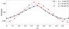 |
Fig. 5 Same as Fig. 2 for an inclination of 70°. |
| In the text | |
Current usage metrics show cumulative count of Article Views (full-text article views including HTML views, PDF and ePub downloads, according to the available data) and Abstracts Views on Vision4Press platform.
Data correspond to usage on the plateform after 2015. The current usage metrics is available 48-96 hours after online publication and is updated daily on week days.
Initial download of the metrics may take a while.