| Issue |
A&A
Volume 591, July 2016
|
|
|---|---|---|
| Article Number | A60 | |
| Number of page(s) | 11 | |
| Section | Astrophysical processes | |
| DOI | https://doi.org/10.1051/0004-6361/201526799 | |
| Published online | 13 June 2016 | |
Master equation theory applied to the redistribution of polarized radiation in the weak radiation field limit
IV. Application to the second solar spectrum of the Na i D1 and D2 lines
LESIA, Observatoire de Paris, PSL Research University, CNRS, Sorbonne Universités, UPMC Univ. Paris 06, Univ. Paris Diderot, Sorbonne Paris Cité, 5 place Jules Janssen, 92190 Meudon, France
e-mail: v.bommier@obspm.fr
Received: 20 June 2015
Accepted: 11 April 2016
Context. The spectrum of the linear polarization, which is formed by scattering and observed on the solar disk close to the limb, is very different from the intensity spectrum and thus able to provide new information, in particular about anisotropies in the solar surface plasma and magnetic fields. In addition, a large number of lines show far wing polarization structures assigned to partial redistribution (PRD), which we prefer to denote as Rayleigh/Raman scattering. The two-level or two-term atom approximation without any lower level polarization is insufficient for many lines.
Aims. In the previous paper of this series, we presented our theory generalized to the multilevel and multiline atom and comprised of statistical equilibrium equations for the atomic density matrix elements and radiative transfer equation for the polarized radiation. The present paper is devoted to applying this theory to model the second solar spectrum of the Na i D1 and D2 lines.
Methods. The solution method is iterative, of the lambda-iteration type. The usual acceleration techniques were considered or even applied, but we found these to be unsuccessful, in particular because of nonlinearity or large number of quantities determining the radiation at each depth.
Results. The observed spectrum is qualitatively reproduced in line center, but the convergence is yet to be reached in the far wings and the observed spectrum is not totally reproduced there.
Conclusions. We need to investigate noniterative resolution methods. The other limitation lies in the one-dimensional (1D) atmosphere model, which is unable to reproduce the intermittent matter structure formed of small loops or spicules in the chromosphere. This modeling is rough, but the computing time in the presence of hyperfine structure and PRD prevents us from envisaging a three-dimensional (3D) model at this instant.
Key words: atomic processes / line: formation / line: profiles / magnetic fields / polarization / radiative transfer
© ESO, 2016
1. Introduction
The aim of this paper is to present a numerical model describing of the so-called second solar spectrum (Stenflo & Keller 1997) of the Na i D1 and D2 lines, making use of the out of local thermal equilibrium (non-LTE) theory for scattering polarization emitted by a multilevel and multiline atom (Bommier 2016). The second solar spectrum is the spectrum of the linear polarization observed on the disk but close to the solar limb. This spectrum reveals a rich structure that is very different from the intensity spectrum and thus likely to provide new information about the medium and, in particular, about its anisotropies and magnetic field via, in particular, the Hanle effect. The Na i D1 and D2 lines linear polarization spectrum presents a particularly rich structure with two polarization far wings on both sides of the polarizable D2 line and also polarization antisymmetrical wings on both sides of the unpolarizable D1 line. Interference between the two upper state wave functions acts as the origin of an envelope of the global polarization profile, as analyzed for the first time by Stenflo (1980) for the Ca ii H and K lines as well as for Na i D1 and D2.
The beautiful linear polarization spectrum of this doublet has been observed several times. It was the cover illustration of the proceedings of an international workshop held in St Petersburg, Russia on 8−12 May 1995, which was reprinted from Fig. 4 of the first paper of this volume (Stenflo 1996). This observation was carried out with ZIMPOL I operating at the Mc Math telescope in April 1995. Later on, the data treatment was reviewed and the spectrum was republished in Fig. 2 of Stenflo & Keller (1997). On this spectrum, a net linear positive polarization peak is clearly visible at the line center of D1. The polarization direction reference (positive polarization) is the direction of the solar limb. This peak represents a formidable challenge for physics because the D1 line is unpolarizable as it has an upper level kinetic momentum J = 1/2, that is too small. Linear scattering polarization reflects the existence of atomic alignment (see for instance Sect 2.3 of Bommier 1996, for definitions) created by the anisotropy of the incident radiation, which may exist only if J ≥ 1. Therefore there were detailed investigations regarding this peak. It was later observed at the Mc Math telescope in March 1998 by Stenflo et al. (2000) at different distances from the solar limb. On the contrary, the net linear polarization in D1 was not observed by Bommier & Molodij (2002), who report observations performed with the THÉMIS telescope in August–September 2000. We repeated these observations several times with THÉMIS and never detected any net linear polarization in D1.
From the theoretical point of view, Casini & Manso Sainz (2005) took all the coherences and interferences into account, but this was for an optically thin model (single scattering) and no global net linear polarization resulted in D1. On the other hand, Landi degl’Innocenti (1998) successfully reproduced the observed spectrum from a metalevel-based theory, except for the net linear polarization peak in D1. Although Landi Degl’Innocenti did not resolve the full, coupled non-LTE problem describing the line formation, he built a successful theoretical spectrum by assuming the presence of alignment in the lower hyperfine levels of the line, computing the resulting linear polarization of the scattered radiation, and integrating it along the line of sight. In the absence of collisions, the metalevel theory for the two-term atom leads to a similar formalism with respect to that recently presented by Casini et al. (2014). Recently, Stenflo (2015) pointed out the possibility that the lower level Zeeman coherences, or interferences between the lower level Zeeman substate wave functions, may play a role in D1 polarization. However, in these two models the lower level alignment or coherences are a priori introduced but not obtained as a solution to the statistical equilibrium for the atomic density matrix.
The aim of the present work is to study partial redistribution (PRD) effects in the Na i D line profiles. In the previous paper of this series (Bommier 2016), we found that PRD, or frequency coherence, results from two different physical mechanisms: first, the Rayleigh/Raman scattering, which induces frequency coherence in the atomic reference frame; and second, Doppler coherence, which relates absorbed and emitted frequencies by an atom of given velocity v, in the laboratory reference frame. The two mechanisms are different, but the relative importance of the coherent phenomenon is governed by related collisional rates. The collisions that weight the PRD are the elastic collisions with hydrogen atoms, in stellar atmopsheres. Rayleigh/Raman scattering is non-negligible when these collisional rates are not larger than radiative rates. Doppler coherence occurs if no collision modifies the atomic velocity during scattering. As shown in Bommier (2016), the velocity-changing collisions form a subclass of the elastic collisions, and, consequently, their rate is very small if the rate of elastic collisions is not large (with respect to the radiative rates). Orders of magnitude are given in Bommier (2016), where we have shown that, in this case, the statistical equilibrium equations have to be resolved for each atomic velocity class. The code we present below is built into this frame. Velocity-independent statistical equilibrium equations in their usual form would not really be self-consistent because this would correspond to high velocity-changing collision rates and, therefore, to very high elastic collisions rates and, in that case, PRD and polarization would become negligible.
In this paper, we present a solution to the full non-LTE problem, by simultaneaously solving the statistical equilibrium equations for the atomic density matrix and the radiative transfer in an iterative manner. In Sect. 2, we describe the physical model we used for the Na atom and for the atmosphere and continuum besides the lines. In Sect. 3 , we describe our code structure. The convergence and acceleration methods are described in Sect. 4. The results are then presented in Sect. 5 and compared with results without hyperfine structure. We conclude in Sect. 6.
2. Physical model
2.1. The model atom
The model atom is represented in Fig. 1 of Kerkeni & Bommier (2002). The level quantum numbers and hyperfine intervals values are given in this figure. Nearly all the density matrix off-diagonal elements are taken into account, connecting all the |n = 3,L,S = 1/2,J,F,M⟩ levels to the |n = 3,L,S = 1/2,J′,F′,M′⟩ levels (only n,L,S are the same on both sides). This results in 640 elements for the atomic density matrix, 64 of which lie in the lower term 32S1/2. When the hyperfine structure is neglected, by artificially assuming a zero nuclear spin I = 0 in place of the real nuclear spin I = 3/2, as we do for some calculations presented below, this element matrix number reduces to 40, 4 of which belong to the lower term. The effect of the transition from the Zeeman effect to the Paschen-Back effect on the level energy differences and proper wavevector components is taken into account as described in Bommier (1980).
The global spontaneous emission probability A(n = 3,L = 1,S = 1/2 → n = 3,L = 0,S = 1/2), which we later denote as A(α2L2S → α1L1S), is taken from the NIST database (old standards) at 6.29 × 10⁷ s-1.
The inelastic collision rates were computed following the method described in Bommier & Sahal-Bréchot (1991) for electron-atom collisions. Nearly at the height where D1 and D2 are formed (see below), i.e., at h = 912 km, where the temperature is T = 5755 K, the electron density Ne = 1.62 × 1011 cm-3 following the VALC quiet atmosphere model (Vernazza et al. 1981), the neutral hydrogen density NHI = 6.63 × 1013 cm-3, the excitation collision probability C(32S1/2 → 32P1/2) is 1.40 × 10² s-1 and C(32S1/2 → 32P3/2) is twice 2.80 × 10² s-1, whereas both de-excitation collision probabilities C(32P1/2 → 32S1/2) and C(32P3/2 → 32S1/2) are 2.98 × 10⁴ s-1, leading to a coefficient for radiative transfer ϵ = C/A of 0.5 × 10⁻³. For the height of the temperature minimum where the D lines begin to form, i.e. at h = 503 km, where the temperature is T = 4400 K, the electron density Ne = 3.04 × 1011 cm-3, the neutral hydrogen density NHI = 2.65 × 1015 cm-3, the excitation collision probability is C(32S1/2 → 32P1/2) is 2.60 × 10² s-1 and C(32S1/2 → 32P3/2) is twice 5.20 × 10² s-1, whereas both de-excitation collision probabilities C(32P1/2 → 32S1/2) and C(32P3/2 → 32S1/2) are 1.99 × 10⁵ s-1, leading to a coefficient for radiative transfer ϵ = C/A of 3 × 10⁻³.
The elastic or quasi-elastic collision rates are those of Kerkeni & Bommier (2002) for the collisions with neutral hydrogen atoms.
For the line widths, as a first step, the interference terms as described in Sahal-Bréchot & Bommier (2014) and recalled in Bommier (2016) were neglected.
The collisional transitions C(32P1/2 ↔ 32P3/2) are fully taken into account. The existence of those transitions between the two fine structure upper levels prevents from any analytical solution to the statistical equilibrium equations. The numerical solution is the only possibility.
2.2. Continuum contribution
The continuum absorption coefficient was evaluated, as in the MALIP code of Landi Degl’Innocenti (1976), by including H− bound-free, H− free-free, neutral hydrogen atom opacity, Rayleigh scattering on H atoms and Thompson scattering on free electrons. This continuum contribution η(c) was added to the line absorption coefficient ηI, which is the diagonal element of the absorption matrix. In this paper, we considered that the continuum polarization is not so well known, in particular the contribution of the Rayleigh scattering on neutral hydrogen, thus we preferred to ignore the continuum polarization. In this respect, and because each process has to be complemented by its opposite process, the contribution of the continuum absorption processes to the emissivity was considered unpolarized and added to the line emissivity εI by assuming LTE as ![\begin{equation} \varepsilon ^{(c)}=\eta ^{(c)}\frac{2h\nu ^{3}}{c^{2}}\frac{1}{\exp \left[h\nu /kT-1\right] }\cdot \end{equation}](/articles/aa/full_html/2016/07/aa26799-15/aa26799-15-eq46.png) (1)
(1)
2.3. Abundance of the atom
The neutral sodium abundance was taken from the subroutine ATMDATb by A.D. Wittmann (Göttingen 1975, by courtesy of IAC). The sodium abundance is 1.91 × 10⁻⁶ times the hydrogen abundance (Grevesse 1984; Thevenin 1989). The partition function for the neutral atom and the two first ions were taken from the subroutine, and the Saha ionization equilibrium was considered to derive the neutral sodium abundance, to which the density matrix was finally normalized for each depth. In order to allow for departures from Saha’s law, the incident radiation temperature was fixed at 5100 K for h> 150 km, where the model electron temperature reached this value, and was set equal to the model electron temperature for h< 150 km.
2.4. Atmosphere model
We used the Maltby et al. quiet sun photospheric reference model (Maltby et al. 1986), extrapolated downward beyond −70 km to −450 km below the τ5000 = 1 level (courtesy of IAC). This model is very close to the VAL-C model of Vernazza et al. (1981) with a deeper extension. We first considered only the photosphere and chromosphere contributions, and we stopped the model at h = 1810 km before the sharp temperature increase that introduces the transition region. This is our 61-point model, but we obtained line intensity profiles with reversal in their center, as visible in Figs. 6 and 12 presented in Sect. 5 below. This reversal in line center is due to the temperature increase with height in the chromosphere.
Such a reversal reflecting the temperature increase was regularly obtained by previous LTE calculations. An example of such reversed profiles from LTE model can be seen in Fig. 6 of Bruls et al. (1992). These authors also present a non-LTE computation, which does not show any reversal in the Na i D line profile. Their model is much richer in atomic levels than ours because it contains all the Na i levels up to n = 7, plus the Na ii continuum, i.e., it is comprised of 17 bound levels plus continuum. Although these authors conclude that “in very first approximation the resonance lines are well described by two-level resonance scattering alone”, the absence of reversal in their non-LTE Na i D line profile is probably due to the large number of upper bound levels included in the statistical equilibrium, and accounting for the Na ii ion first level. However, their theoretical non-LTE profile, though not reversed, is clearly deeper than the observed profile, as is visible for instance in the second solar spectrum atlas (Gandorfer 2000), or in Fig. 7 of Uitenbroek & Bruls (1992), who employ nearly the same atomic model.
The recent adaptation of this model, proposed by Leenaarts et al. (2010) and Rutten et al. (2011), consists in resuming all the Na i levels higher than those connecting the D lines to a single artificial level with well-adapted transition, ionization, and recombination probabilities to model the “photon suction” population flow that tends to populate the Na i ground level from the ion via the upper levels. In the following, we develop an alternative method to model the observed Na i line profile.
Other investigators have generated more recent non-LTE models that take polarization into account. As with our model, these models include fewer bound levels than the model by Bruls et al. (1992) because they are two-term models. Instead, Belluzzi & Trujillo Bueno (2013) for Na i and Anusha et al. (2010) for Ca i resonance line, apply the MCO (also known as FAL-X) atmosphere model of Avrett (1995). Smitha et al. (2013), who study Ba ii resonance line, elaborated on an even cooler atmosphere model than FAL-X. The FAL-X atmosphere model, already known to “give a good fit to the full range of mean CO line profiles, but conflic[ting] with other observations of average quiet regions” (Avrett 1995), is characterized by the fact that the temperature minimum occurs much higher than in VAL-C, at about 1000 km for FAL-X instead of 500 km for VAL-C. The atmosphere model that is cooler than FAL-X is also found to be better for fitting the observed center-to-limb behavior of the Ca i resonance line (Supriya et al. 2014). However, Faurobert et al. (2009) do not find any significant difference between using FAL-C and FAL-X for their model describing the Ba ii D2 line polarization near the solar limb. Their model atom is two-term also, with the addition of the metastable level in between for Ba ii. We note that all of these authors (except Faurobert et al. 2009) plot only Q/I behaviors but not pure intensity profiles.
We first evaluated the LTE line formation height of the Na i D lines, under the hypotheses previously described in Sects. 2.2 and 2.3, as follows. To obtain this preliminary result, the line center optical depth grid was scaled to the continuum optical depth grid using the respective absorption coefficients and assuming Saha-Boltzmann populations. The continuum optical depth grid was that provided with the atmospheric model and the transfer equation was not explicitly solved again. The height of formation of the line center was then determined as follows. Given the grid of line center optical depths, the height of formation of the line center is that for which the optical depth along the line of sight is unity (Eddington-Barbier approximation), i.e., that for which τ/μ = 1, where τ is the line center optical depth along the vertical and μ the cosine of the heliocentric angle θ (here supposed to be 0). We thus obtained quiet sun LTE line center formation heights of 533 km for Na I D1 and 604 km for Na I D2 above the τ5000 = 1 level. These heights are just above the temperature minimum of VAL-C and in good agreement with Fig. 6 of Bruls et al. (1992).
It is thus obtained that the Na i D lines when considered in LTE form just above the temperature minimum of the VAL-C model, but much below the temperature minimum of FAL-X. It may be concluded that using FAL-X would avoid the temperature minimum being included in the line formation depth range. Following the previously cited authors, we tried the FAL-X model and also the similar FCHHT models by Fontenla et al. (20091; thanks to K.N. Nagendra). We, however, also obtained a reversal in the intensity of our Na i D line profiles possibly because their temperature minimum is steeper as it is higher in the atmosphere or because of the much higher formation heights we obtain in non-LTE (see Fig. 9). We were, in addition, mainly unsatisfied that the FAL-X model corresponds to a cooler medium than the average quiet sun we were studying. We then rather investigated another idea, as follows.
Chromosphere images, taken in the Hα line out of disk center (thanks to an image acquired by Luc Rouppe van der Voort and Michiel Van Noort at the Swedish Solar Telescope (SST) on 4 October 2005, and shown by M. Carlsson at a THÉMIS workshop at Meudon Observatory on 19−21 May 2010), show that the atmosphere becomes intermittent above a certain height, i.e., it is comprised of small matter loops or spicules separated by much more void atmosphere. Atmosphere models, however, are built from spectral line analysis because the lines are formed where the matter is. Thus we think that the model reflects only a part of the space above a certain height. In other words, above a certain height there is mainly no matter along the line of sight. The problem is to determine this height. Our guess is that this height is the VAL-C temperature minimum height. We thus limited our model to the temperature minimum height h = 503 km. Thus, the reversal in line center disappeared and the Na i D1 and D2 intensity line profile was obtained in a much better agreement with the observations as visible in Figs. 5 and 10 in Sect. 5 below. This is our 48-point model.
We know that in the full VAL-C 61-point model, there are points well above h = 503 km, where the contribution function in the Na i D lines is not negligible at all, as visible in Fig. 9. As a consequence, the line center optical depth is high at h = 503 km in the full model. By cutting our atmosphere model at h = 503 km, we do not perform a questionable approximation by suppressing non-negligible contributions. However, we want to built a new 1D model that takes into account as much as possible, in the 1D frame, the fact that it seems the chromosphere is made of intermittent matter. Because our model is only 1D, it is unfortunately thus unable to take into account intermittent matter under the form of loops or spicules. Building a 3D model capable of this, on the theory presented below, would certainly be the best way to proceed, but this is not possible with present computers.
Similar models were considered in the past. Bruls et al. (1992) also consider the HOLMUL model (Holweger & Mueller 1974) in which there is no temperature minimum and no reversal in the line profiles computed within the LTE hypothesis. In this model, the temperature is assumed to decrease indefinitely with height. Considering that such a model was not used anymore and also considering the intermittent nature of the chromosphere matter, as revealed by recent images such as those of the SST cited above, we thus preferred to consider a model limited to the photosphere. This model is very close to the T5780 model (Edvardsson et al. 1993) used by Carlsson et al. (1992) and Carlsson et al. (1994).
3. Code structure
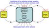 |
Fig. 1 Flow chart of the new code XTAT, resolving both statistical equilibrium and radiative transfer equations for a multilevel-multiline atom, including the redistribution, polarization, and magnetic field. |
The code is built about the statistical equilibrium code developed following Bommier (1980). This code does not use the tensorial algebra for developing the atomic density matrix, which is developed over the dyadic basis instead. The reason is that the code is aimed to be valid under the incomplete Paschen-Back conditions (or the analogous conditions for the hyperfine structure). As already explained in Bommier (1980), in this case the number of possibly non-zero matrix elements developed on the tensorial basis is not reduced with respect to the number of elements when the matrix is projected onto the dyadic basis and the transformation of the equations into the tensorial basis is a supplementary effort leading to more complex equations.
The novelty of the present formalism is that the density matrix now depends on the atomic velocity, and that the statistical equilibrium has to be resolved for each atomic velocity class. It is assumed that the different velocity classes are not coupled, which is valid provided that the velocity changing collisions remain weak, which is expected in the solar atmosphere. We have 640 density matrix elements for each velocity class, leading to a 640 × 640 system of linear equations to be resolved. The number of elementary velocities is 48 in our computation, and introducing couplings would instead lead to a 48 × 48 × 640 × 640 system, which is too large for the present computers. In Sect. 3.2 below, we describe how the velocity vector is discretized and how the numerical integrations are performed. The statistical equilibrium is resolved for each velocity class and then the contribution of this velocity class to the radiative transfer equation coefficients is computed, which is finally integrated over the atomic velocities. Then, the radiative transfer equation is integrated along each internal ray path to evaluate the radiation incident on each internal level of the atmosphere, which is assumed to be plane parallel. The code is 1D. Once this incident radiation is computed, the statistical equilibrium equations for the atomic density matrix may be solved again; this is the next iteration step. We have thus developed an iterative resolution of the coupled statistical equilibrium and radiative transfer equations, which is of the lambda-iteration type. This is known to require acceleration techniques for convergence, the effect of which is described in Sect. 4.
The flow-chart of the total iterative code is presented in Fig. 1. The code name is XTAT, for “statistical equilibrium”.
3.1. Initialization and boundary conditions
For the calculations presented in this paper, the density matrix was initialized as an “ultracold” atom, i.e., with all sublevels of the lower term 32S1/2 equally populated and the populations and coherences of all sublevels of the upper terms 32P1/2 and 32P3/2 set to zero. A different initialization was attempted with the sublevel populations given by the Boltzmann law and all coherences (off-diagonal elements) set to zero. Generally, in non-LTE the excited level populations are smaller than the Boltzmann populations, but larger than zero, so that these two initialization schemes represent opposite starting conditions with respect to the final result. On trial cases, the same final results were reached from these two opposite starting conditions, thus validating this initialization.
An incident radiation was assumed to be present below the atmosphere. The intensity radiation was assumed to be given by the Planck function taken at the electron temperature of the lower point of the atmosphere. However, this radiation was assumed to be anisotropic by applying the diffusion approximation (Milahas 1978, p. 51, Eq. (2−90a)).
3.2. Integrations
3.2.1. Radiative transfer equation integration
The radiative transfer equation was integrated along each internal line of sight, following the short characteristics method renewed by Ibgui et al. (2013). As mentioned by these authors, Taylor expansions up to the third order were used instead for optical depth differences smaller than 5 × 10⁻².
In the case of polarized radiative transfer, absorption of the Stokes parameters is described by an absorption matrix. However, in a first step, no magnetic field was assumed in our calculation, thus resulting in a diagonal absorption matrix with diagonal element ηI. The lower level alignment is also ignored for this, which is very small (Kerkeni & Bommier 2002). Thus, in a first step no matrix inversion was required. This could be implemented in the future for modeling the presence of a magnetic field, in particular applying matricial techniques developed by Bommier & Landi Degl’Innocenti (1996).
3.2.2. Numerical integrations over velocities or frequencies and directions
We were limited to rather small numbers of moduli and angles owing to lack of sufficient computer time. All the integrations were performed by applying Gauss-type integration methods with abscissae and weights (see for instance Press et al. 1989). We considered six velocity moduli. The integration on these moduli for the radiative transfer equation coefficients, was performed by applying the generalized Gauss-Hermite integration, which is adapted to integrate functions proportional to v2exp(−v2), as is the Maxwellian velocity distribution function. However, the generalized Gauss-Hermite integral assumes that the integral limits extend from −∞ to + ∞, thus introducing unphysical negative velocity moduli. However, the Doppler effect induced by such moduli is not yet unphysical; in the Doppler effect expression, a negative velocity modulus corresponds to a velocity of same absolute modulus but opposite direction. We considered two inclinations and four azimuths for the directions, velocities, and radiation, and we applied the usual Gauss-Legendre method for computing the corresponding integrals. The Gauss-Legendre abscissae for the azimuth integration are not found to be equally spaced between 0 and 2π, but we found that the introduction of the negative velocity moduli fortunately compensates for this inequality. In the end, this leads to much better accuracy than applying the usual trapezoidal integration, which is known to be poorly convergent. We obtain these results with trials on larger numbers of integration abscissae, which we were later obliged to reduce for the final computation. By considering an even velocity modulus number, six, we avoided the zero velocity, which is without any direction and could have raised problems for the direction integrals.
Frequency integration along the line profile is present in the statistical equilibrium equation coeffcients for the atomic density matrix. Because these equations are to be resolved for each atomic velocity class, this profile is the Lorentz profile, whose width is given by the sum of the two connected level inverse lifetimes, plus an eventual interference term, which is of the same order of magnitude (see Sect. 3.4 of Bommier 2016). Under solar atmosphere conditions, the natural and collisional width are very small with respect to the width of the solar line under study. This implies a difficulty in defining enough close together frequency abscissae that are able to recover each Lorentz profile and also spread over the whole solar line profile. Instead, we neglect the variation of the solar line spectrum along the Lorentz profile, which we replace by a delta function in the calculation.
An analogous difficulty appears when integrating the radiative transfer equation coefficients on the velocity distribution. For each velocity, the absorption and emission coefficients are also frequency-dependent along a Lorentz profile. The number of velocities in our computation, however, is much too small to sufficiently cover all the Lorentz profiles in the velocity distribution function integration because the Lorentz profile widths are small with respect to the Doppler width. We instead used Voigt profiles with Doppler width taken at the conditions of the atmosphere upper limit in the radiative transfer equation coefficient computation to compensate for this deficiency. We applied this rough approximation to all the Φba profiles of the coefficients (see Sect 3.3 of Bommier 2016). For the second term of the emissivity  where a Φca profile appears (with c = a in the case of the Na i D lines), this profile has been approximated by a delta function, assuming that in the case of the Na i D lines, the lower levels are infinitely sharp (the broadening effect of the radiative absorption is neglected).
3.3. Parallelization
Our XTAT code was parallelized in the hybrid MPI and OpenMP scheme. The MPI parallelization was applied to the depth discretization in the 1D atmosphere because the incident radiation is computed at each depth as an initial condition for solving the statistical equilibrium equation at this depth and then evaluating the radiative transfer equation coefficients, which are then gathered from the different depths and broadcasted to each node for recomputing the incident radiation by integrating the radiative transfer equation.
Our atmosphere model is 48 or 61 depths large. We first expand this grid into 256 equally spaced grid points by applying a cubic spline interpolation. These 256 depths are each treated by 256 computer nodes running in parallel and coupled with the MPI software.
At each depth, the loops on velocities, for statistical equilibrium resolution for each atomic velocity and for the velocity integration for each radiative transfer equation coefficients, are treated as an OpenMP loop, with shared access to the unique radiative transfer equation coefficient table stored in each node (shared memory). There are a priori three loops on velocity moduli, inclinations, and azimuths. These three loops are merged into a single loop, which is OpenMP parallelized, for the statistical equilibrium resolution and for each radiative transfer equation coefficient calculation. The code was run in the Blue-Gene/Q machine of the IDRIS center in Orsay (France), which is a massively parallel computer. Each node has 16 cores, and each core can support four different threads, a feature that we used. Thus the OpenMP loop on the 6 × 2 × 4 velocities was spread on the 64 threads of each node.
The computing time was on the order of 12 h for one iteration step, which is on the order of 50 000 h run in total by the 4096 cores used at a time.
4. Convergence and acceleration
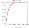 |
Fig. 2 Convergence of the D2 line center intensity, as a function of the iteration step number for the atmosphere model limited at the temperature minimum (48-point model), and neglecting the hyperfine structure and PRD for a quicker computation. |
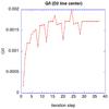 |
Fig. 3 Convergence of the D2 line center polarization as a function of the iteration step number, for the atmosphere model limited at the temperature minimum (48-point model). |
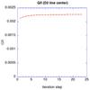 |
Fig. 4 Convergence of the D2 line center polarization as a function of the iteration step number, for the atmosphere model not limited at the temperature minimum (61-point model). |
The iterative method outlined in Fig. 1 is of the lambda-iteration type. This kind of method is known to slowly converge. More precisely, the number of iteration steps required for convergence is on the order of the largest inverse collisional to radiative ratio 1 /ϵ of the problem under study. As stated above, we have ϵ ≈ 10-3, so that the number of steps required to get convergence would be on the order of one thousand. This is what we obtained, for convergence of the intensity at line center. We experienced this convergence in the CRD case (i.e. by ignoring the order-4 second term of the emissivity) and without hyperfine structure (by artificially putting I = 0 for the nuclear spin). In this case, the computations are much quicker and were performed in the local computing center MESOPSL. The convergence is plotted in Fig. 2.
However we are interested in the line center polarization, which is not the intensity itself, but the ratio of Stokes parameters Q/I; we obtained that the convergence of this ratio behaves very differently with respect to the convergence of the intensity. In Fig. 3, which is computed with the 48-point model atmosphere, it can be seen that the line center polarization convergence is correctly reached from 15 steps. This is also largely the case for Fig. 4 computed with the 61-point model atmosphere. The physical explanation lies in the fact that the polarization (the ratio of Stokes parameters) is not sensitive to the same physical parameters as the intensity (the Stokes parameters themselves). The polarization reflects the radiation anisotropy in the medium, but not the radiation itself.
However, this does not prevent us from examining the effect of the different acceleration methods proposed in the literature.
4.0.1. Preconditioning
A series of methods have been developed under the name of preconditioning. This consists in letting unresolved, in the radiative transfer integration for computing the incident radiation, the population of the point under interest itself, and to introduce it as an unknown in the statistical equilibrium equation to be resolved. This procedure, which was described by Rybicki & Hummer (1991, 1992) for a multilevel atom, could obviously be generalized to polarization and Zeeman sublevels, but the implementation would be a rather hard work. In addition, we observed that we solve the statistical equilibrium equation for each atomic velocity class. We have 6 × 2 × 4 = 48 velocities in our computation and we would precondition only one of these 48 velocities at a time, which is a small ratio. Rybicki & Hummer (1992, p. 211) state that “the preconditioning of some [several] terms may have little effect on the convergence rate”, which we understood also as the more levels are involved, the less efficient the method. We prepared a simpler code with only one radiation frequency submitted to Rayleigh scattering to investigate this point. Numerical integrations were performed on the radiation directions and the preconditioning was performed one direction only at a time. We observed that in such a case the acceleration is inefficient, so that we finally did not apply this method to our full code.
Uitenbroek (1989) developed a method for taking PRD effects into account in multilevel NLTE modeling based on the redistribution functions by Hubený et al. (1983). This formalism does not contradict ours because Eq. (10) of Uitenbroek (1989) with the emissivity comprised of two contributions, is the same as ours for a two-level atom (Bommier 1997a). In contrast, our approach is more self-consistent. We renewed the formulation by showing that the statistical equilibrium equations have to be resolved for each atomic velocity class. Our approach with the coupled resolution of radiative transfer and statistical equilibrium does not use any redistribution function. These functions are products of scattering modeling on a two-level atom or even a three-level atom in the case of Raman scattering, where the scattering initial and final levels are different. These functions are first derived in the atomic frame (Omont et al. 1972) for an atom of given velocity. The average on atomic velocities is performed later, thus there is no contradiction with our approach, but the redistribution functions are two- or three-level atom tools, so that their inclusion in multilevel non-LTE modeling is less self-consistent than our approach. Uitenbroek (2001) successfully applied full preconditioning (i.e., preconditioning of all the atomic levels at a given depth at a time) for convergence acceleration, but in an unpolarized and angle-averaged formalism, which much reduced the number of independent quantities determining each radiation frequency. Thus it can be understood that preconditioning was efficient for Uitenbroek (2001). Miller-Ricci & Uitenbroek (2002) also considered the cross redistribution (XRD), which is the Raman scattering with different initial and final levels for the coherent scattering, which we considered as well. Our method, with the velocity-dependent atomic density matrix in the statistical equilibrium equations, is more self-consistent.
4.0.2. Ng acceleration
The other series of method is called Ng acceleration. We followed its description by Olson et al. (1986) for application. The method was applied to each radiative transfer equation coefficient εI...V,ηI...V,ρQ...V. As recommended by Olson et al. (1986), we applied weights. We applied the same weight for all the Stokes parameters of a series, i.e. we applied  for all εI...V, and
  for all ηI...V and ρQ...V in contrast to Faurobert-Scholl et al. (1997), who applied weight to the intensity coefficients (i.e. those with index I) but no weight to the others. We think that all the coefficients are scaled by the intensity coefficient, which can be used as a normalization.
Figure 3 shows that the result of this acceleration technique seems to be random. As recommended by Olson et al. (1986), the technique was applied after three steps of normal iteration. This technique is an extrapolation based on the assumption that the system has a linear behavior. This is the case for the two-level atom system and Figs. 6 and 7 of Faurobert-Scholl et al. (1997) show that in this case the acceleration is very efficient. But ours is not the two-level case. In the two-level case, there is no resolution of the statistical equilibrium equation because there is only one equation that is resolved as soon as it is written, whereas in the multilevel case the solution to the statistical equilibrium system of equations is highly nonlinear in function of the coefficients of the equations. We assign this nonlinearity to be at origin of the random behavior of the acceleration as visible each of four steps of Fig. 3. Once observed the random behavior of the result, we preferred to abandon this acceleration method for the last iteration steps of the calculation with the 48-point model atmosphere reported in Fig. 3. For the calculation with the 61-point model atmosphere, which was performed later, we did not apply the method.
4.0.3. Convergence in the line wings
The convergence in the line wings is much slower, and was not reached in the results presented in this paper. As stated above, we developed a smaller test code with only one radiation frequency submitted to Rayleigh scattering to investigate this convergence. This situation approaches that of the line far wings. At each atmosphere depth the integration on the radiation directions was performed numerically. Not only did we not reach convergence with a much larger number of iteration steps, but we observed a very slow propagation of the radiation through the atmosphere along depth. This is the case even though the diffusion approximation of Milahas (1978, p. 51, Eq. (2− was introduced, which takes into account the radiation anisotropy at large depths and gives an average propagation directed upward. We also observed that the presence of a LTE contribution to the radiation introduced by adding an ϵBν contribution (Planck function times an artificial collisional to radiative de-excitation ratio), together with weighting the Rayleigh scattering with (1−ϵ; same ϵ), does not permit us to reach the convergence. We think that methods other than lambda-iteration have to be developed for this multilevel problem to reach convergence in the far wings. We decided, however, to publish the present results as a working step.
Other authors developed iterative resolution methods for non-LTE radiative transfer taking partial redistribution (PRD) into account. Sampoorna et al. (2010) assumed axial symmetry about the vertical of the 1D atmosphere, however. This method was later applied by Belluzzi & Trujillo Bueno (2012, 2013), Belluzzi et al. (2012). As a result of this assumption, there is no integral on azimuths. Aiming to introduce a magnetic field not necessarily vertical or random in the model, we did not perform this assumption. As a consequence, we have azimuth as a variable and we have to perform integrations on this variable. On the other hand, Nagendra et al. (2002) developed a solution technique in three steps: starting from an unpolarized PRD solution, the polarization is first added but angular averaged, and the angular dependence is introduced in the third step. This paper introduces a nonvertical magnetic field in the model, following the redistribution functions of Bommier (1997b) in the presence of a magnetic field. All these methods are however strongly limited to two-level or two-term model atom. In the present paper, our multilevel theory is able to take into account the presence of any magnetic field, but for the first calculation presented in this paper, a zero magnetic field was assumed.
5. Results
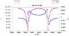 |
Fig. 5 Emergent intensity and linear polarization parallel to the solar limb for the atmosphere model limited at the temperature minimum (48-point model). The number of iterations steps is 37. The limb distance is set at 4.1 arcsec (μ = cosθ = 0.092) for comparison with the observations by Bommier & Molodij (2002). |
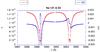 |
Fig. 6 Emergent intensity and linear polarization parallel to the solar limb for the atmosphere model not limited at the temperature minimum (61-point model). The number of iterations steps is 23. The limb distance is set at 4.1 arcsec (μ = cosθ = 0.092) for comparison with the observations by Bommier & Molodij (2002). |
The computed Na i D1 and D2 second solar spectrum is presented in Fig. 5 for the 48-point atmosphere model, which is limited to the temperature minimum, corresponding to the maximum atltitude at which we expect the atmosphere to be continuous. A qualitative but good agreement is visible in line centers with the observations for D1 and D2, except that the net linear polarization peak in D1 is not retrieved. As obtained by Casini & Manso Sainz (2005) and Landi degl’Innocenti (1998), D1 is globally antisymmetrical without any net linear polarization. Interestingly, a sharp structure appears in the very center of D1 that is very analogous to what was observed by Bommier & Molodij (2002, Figs. 2, 3). The effect of a line-of-sight velocity gradient, which is able to destroy profile symmetries, will be investigated in future work.
In the wing, convergence is not reached. A wing peak in the polarization profile is visible in the red wing of D2, analogous to the observations, but the similar peak of the observations in the blue wing is absent from the calculated profile and the bumps in the far wings of the blue and red sides of D1 are also absent from the calculated profile.
Figure 6 reports the result for the 61-point atmosphere model, which is the same atmosphere without any limitation to temperature minimum. The whole chromosphere (ignoring its intermittency) is included up to the basis of the transition region. In this case, it is visible in the figure that the line intensity profiles show a reversal at center that we assign to the presence of the temperature increase above the temperature minimum in the model atmosphere.
5.1. Contribution functions and formation heights
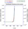 |
Fig. 7 Contribution functions for Stokes I et Q at line center for the atmosphere model limited at the temperature minimum (48-point model). The maximum height of the model is h = 503 km. The plot is zoomed to about this value. |
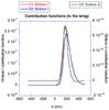 |
Fig. 8 Contribution functions for Stokes I et Q in the far wing for the atmosphere model limited at the temperature minimum (48-point model). The maximum height of the model is h = 503 km. The wing frequency is that of the polarization maximum in the red wing of D2 and the analogous frequency in the red wing of D1. |
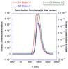 |
Fig. 9 Contribution functions for Stokes I et Q at line center for the atmosphere model not limited at the temperature minimum (61-point model). The D1 line center Stokes I contribution function reaches a maximum at 6.9 × 10⁻⁸ for the height h = 888 km. The D2 line center Stokes I contribution function reaches a maximum at 5.3 × 10⁻⁸ for the height h = 968 km. The D2 line center Stokes Q contribution function reaches a maximum at 1.18 × 10⁻¹⁰ for the same height h = 968 km. |
The contribution functions we present here are numerical contribution functions, given by 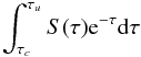 (2)for the contribution of the interval between points u and c, which results in numerical form (short characteristics method) as
 ![\begin{equation} \left[\alpha {\rm S}_{u}+\beta {\rm S}_{c}+\alpha ^{\prime }\left. \frac{\mathrm{d}S}{ \mathrm{d}\tau }\right\vert _{u}+\beta ^{\prime }\left. \frac{\mathrm{d}S}{ \mathrm{d}\tau }\right\vert _{c}\right] \mathrm{e}^{-\tau _{c}}, \end{equation}](/articles/aa/full_html/2016/07/aa26799-15/aa26799-15-eq102.png) (3)following Eq. (14a) of Ibgui et al. (2013), and where τc (resp. τu) is the optical depth at point c (resp. u). The contribution function is assigned to point c (see Fig. 1 of Ibgui et al. (2013) for point definition). All the atmosphere points are equidistant. The source function S is given by εI/ηI for intensity Stokes I and εQ/ηI for polarization Stokes Q.
(3)following Eq. (14a) of Ibgui et al. (2013), and where τc (resp. τu) is the optical depth at point c (resp. u). The contribution function is assigned to point c (see Fig. 1 of Ibgui et al. (2013) for point definition). All the atmosphere points are equidistant. The source function S is given by εI/ηI for intensity Stokes I and εQ/ηI for polarization Stokes Q.
Our atmosphere model was finally comprised of 256 equally spaced grid points and we plot each depth contribution to the emergent intensity I in D1 and D2, and Stokes Q of the polarizable D2. Figure 7 gives the contribution functions in the line center for the 48-point model atmosphere, which is limited to the temperature minimum. In this case, the line centers are not completely formed at the height where the model is cut in a rough manner resulting from the inadequate 1D adopted structure to account for the matter-intermittent structure of the chromosphere. Along with the lack of 3D modeling, this can explain why the line center theoretical polarization only matches the observations qualitatively.
The contribution function in the far wings, with the same atmosphere model, is given in Fig. 8. The maximum D1 intensity I formation height is 181 km, whereas the maximum formation height for D2 is 192 km for I and 170 km for Q. All these altitudes are then found very close together.
Figure 9 gives the contribution functions for the more complete 61-point model atmosphere. The figure shows that the maximum D1 intensity I formation height is 888 km, whereas the maximum formation height for D2 I and Q is 968 km. The maximum formation height is the same for both D2 I and Q.
5.2. Results with fine structure only
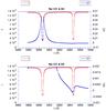 |
Fig. 10 Same as Fig. 5, but with fine structure only and without taking the hyperfine structure into account. The atmosphere model limited at the temperature minimum (48-point model). The number of iterations steps is 175. The lower plot is a zoom on the polarization scale to make the D1 polarization visible. |
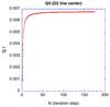 |
Fig. 11 Convergence of the D2 line center polarization as a function of the iteration step number in the case of Fig. 10 (48-point model). |
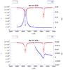 |
Fig. 12 Same as Fig. 6, but with fine structure only and without taking the hyperfine structure into account. The atmosphere model is not limited at the temperature minimum (61-point model). The number of iteration steps is 158. The lower plot is a zoom on the polarization scale to make the D1 polarization visible. |
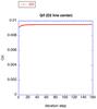 |
Fig. 13 Convergence of the D2 line center polarization as a function of the iteration step number, in the case of Fig. 12 (61-point model). |
For comparison, we show in Figs. 10−13 what the results would be in the absence of hyperfine structure for the two 48-point and 61-point models. To do this, we arbitrarily assumed a zero nuclear spin I = 0 in place of the real nuclear spin I = 3/2. Figures 10 and 12 show that the line polarization far wings are much stronger than in the hyperfine structure case, but are now too strong with respect to the observations. However, as mentioned in Sect. 4.0.3, the convergence is probably not reached there. This reveals, however, that the method is potentially capable of partial redistribution and far wings modeling.
As in the hyperfine structure case, accounting for the temperature increase above the temperature minimum leads to a reversal in the intensity profile, as shown in Fig. 12, which is not present when the atmosphere model is limited to the temperature minimum as in Fig. 10. The convergence of the polarization at line center given in Figs. 11 and 13 is analogous to that of the hyperfine structure case.
5.3. Velocity distribution in the excited states
The Na i global velocity distribution function f(v) (i.e. ignoring the internal state) has been assumed to be Maxwellian. The level velocity distribution in the (αJM) level is  (4)The density matrix ρ(v,t) was normalized to the neutral sodium abundance as defined in Sect. 2.3. As the lower term total population is much larger than the upper term population, the lower level velocity distribution function is found to be very close to the Mawxellian. This is not the case for the upper level velocity distribution function, however. At the temperature minimum altitude h = 503 km (in the 48-point model atmosphere), we obtain a departure of 5% from the Maxwellian in the excited levels. Higher in the atmosphere, i.e., in the chromosphere, at h = 970 km and h = 1810 km (in the 61-point model atmosphere), the departure reaches 20%. We measure this departure as the standard deviation, normalized to the average value, of the ratio between the upper and lower level populations as a function of the atomic velocity. This non-negligible departure confirms the necessity of resolving the statistical equilibrium equations for each velocity class.
6. Conclusion
We have presented a model describing the linear polarization of the Na i D1 and D2 lines as observed on the solar disk close to the limb, as the first application of a multilevel general theory of radiation scattering presented in the preceding paper of this series (Bommier 2016) . This theory aims to describe both coherent (or Rayleigh/Raman) scattering and incoherent (or resonant) scattering, wich are responsible for far wings and line core polarization, respectively. Accounting for coherent scattering is often referred to as the partial redistribution effect (PRD). Our theory was developed in the frame of the atomic density matrix formalism. The principles and main steps of the development are those of Bommier (1997a) and are based on overcoming of the Markov (or short-memory) approximation. This improvement enables us to account for the past processes as a line-broadening mechanism. In Bommier (2016), we recalled the main steps and principle of our improved method and, in particular, how we expressed this improvement as a series development, whose summation is known, thus leading to an unperturbative summed final result. In the first paper of this series, Bommier (1997a), we provided the final equations, statistical equilibrium and radiative transfer, for a two-level atom with unpolarized lower level. In Bommier (2016), we presented the general equations for the case of a multilevel atom.
The present paper is an application of this theory to the model describing the second solar spectrum of the Na i D1 and D2 lines. The solution method is iterative of the lambda-iteration type. The method is not accelerated by the usual techniques developed for this purpose due to, in particular, the nonlinearity of the statistical equilibrium of a multilevel atom with respect to the two-level or two-term atom without lower level polarization. This is also as a result of the large number of quantities that determine the radiation at each depth because we did not assume any symmetry for our problem, with the aim of introducing a nonvertical magnetic field in future works. Thus, numerical azimuths are present in the integrations. Also, we have shown in Bommier (2016) that the statistical equilibrium has to be resolved for each atomic velocity class. Thus, each level population (or inter-level coherence) is not a single number, but a distribution in function of the atomic velocities that is discretized for computation. Thus this large number of independent quantities makes the usual technique of preconditioning inefficient.
We find that the convergence is yet to be reached in the line far wings, so that their observed shape is not reproduced in that region. The resolution of this problem will probably lie in finding a noniterative solution method, or applying a Monte-Carlo method, which is an ambitious objective for a future work. Alternatively, we could take advantage of the polarization degree remaining weak so that iteration could be first performed ignoring polarization, which would reduce the number of unknowns. Once the convergence is reached without polarization, the polarization could be introduced and convergence expected in a few steps. In addition, to improve convergence, less than 256 depth points could be assumed in the first step. The atmosphere would be first discretized on a coarse grid and later iterpolated to a finer grid after convergence.
In addition, a 1D atmosphere model was assumed and this is probably seriously inconvenient for those lines that are formed in the chromosphere because the chromosphere is probably a matter-discontinuous medium comprised of small loops or spicules. The computing time in the presence of hyperfine structure and PRD, however, prevents us from envisaging a 3D model. In this respect, we limited the atmosphere model to the continuous part of the atmosphere, which we assigned to be limited to the temperature minimum level. This rough structure of our atmosphere model is probably the reason why the line center polarization profiles are only reproduced somewhat qualitatively. However, a central sharp structure is obtained in the center of D1, as in the observations by Bommier & Molodij (2002). The polarization profile of D1 is found globally antisymmetric. No net linear polarization is obtained in D1, as obtained by Casini & Manso Sainz (2005) and Landi degl’Innocenti (1998); this is in contrast to the observations by Stenflo (1996), Stenflo & Keller (1997), Stenflo et al. (2000) and in agreement with the observations of Bommier & Molodij (2002). Further investigation is envisaged concerning the effect of a line-of-sight atomic velocity gradient as a possible source of profile antisymmetry breaking.
Also available at http://vizier.cfa.harvard.edu/viz-bin/VizieR?-source=J/ApJ/707/482
Acknowledgments
This work was granted access to the HPC resources of MesoPSL financed by the Region Ile de France and the project Equip@Meso (reference ANR-10-EQPX-29-01) of the Investissements d’Avenir program supervised by the Agence Nationale pour la Recherche. Besides, this work was granted access to the HPC resources of IDRIS under the allocations 2014-i2015047205 and 2015-i2015047205 made by GENCI. The author is grateful to the referee, H. Uitenbroek, for helpful suggestions.
References
- Anusha, L. S., Nagendra, K. N., Stenflo, J. O., et al. 2010, ApJ, 718, 988 [NASA ADS] [CrossRef] [Google Scholar]
- Avrett, E. H. 1995, in Infrared Tools for Solar Astrophysics: What’s Next?, eds. J. R. Kuhn & M. J. Penn (Singapore: World Scientific), 303 [Google Scholar]
- Belluzzi, L., & Trujillo Bueno, J. 2012, ApJ, 750, L11 [NASA ADS] [CrossRef] [Google Scholar]
- Belluzzi, L., & Trujillo Bueno, J. 2013, ApJ, 774, L28 [NASA ADS] [CrossRef] [Google Scholar]
- Belluzzi, L., Trujillo Bueno, J., & Štěpán, J. 2012, ApJ, 755, L2 [NASA ADS] [CrossRef] [Google Scholar]
- Bommier, V. 1980, A&A, 87, 109 [NASA ADS] [Google Scholar]
- Bommier, V. 1996, Sol. Phys., 164, 29 [NASA ADS] [CrossRef] [Google Scholar]
- Bommier, V. 1997a, A&A, 328, 706 [NASA ADS] [Google Scholar]
- Bommier, V. 1997b, A&A, 328, 726 [NASA ADS] [Google Scholar]
- Bommier, V. 2016, A&A, 591, A59 [NASA ADS] [CrossRef] [EDP Sciences] [Google Scholar]
- Bommier, V., & Molodij, G. 2002, A&A, 381, 241 [NASA ADS] [CrossRef] [EDP Sciences] [Google Scholar]
- Bommier, V., & Sahal-Bréchot, S. 1991, Ann. Phys., 16, 555 [Google Scholar]
- Bommier, V., & Landi Degl’Innocenti, E. 1996, Sol. Phys., 164, 117 [NASA ADS] [CrossRef] [Google Scholar]
- Bruls, J. H. M. J., Rutten, R. J., & Shchukina, N. G. 1992, A&A, 265, 237 [NASA ADS] [Google Scholar]
- Carlsson, M., Rutten, R. J., & Shchukina, N. G. 1992, A&A, 253, 567 [NASA ADS] [Google Scholar]
- Carlsson, M., Rutten, R. J., Bruls, J. H. M. J., & Shchukina, N. G. 1994, A&A, 288 [Google Scholar]
- Casini, R., & Manso Sainz, R. 2005, ApJ, 624, 1025 [NASA ADS] [CrossRef] [Google Scholar]
- Casini, R., Landi Degl’Innocenti, M., Manso Sainz, R., Landi Degl’Innocenti, E., & Landolfi, M. 2014, ApJ, 791, 94 [NASA ADS] [CrossRef] [Google Scholar]
- Edvardsson, B., Andersen, J., Gustafsson, B., et al. 1993, A&A, 275, 101 [NASA ADS] [Google Scholar]
- Faurobert, M., Derouich, M., Bommier, V., & Arnaud, J. 2009, A&A, 493, 201 [NASA ADS] [CrossRef] [EDP Sciences] [Google Scholar]
- Faurobert-Scholl, M., Frisch, H., & Nagendra, K. N. 1997, A&A, 322, 896 [Google Scholar]
- Fontenla, J. M., Curdt, W., Haberreiter, M., Harder, J., & Tian, H. 2009, ApJ, 707, 482 [NASA ADS] [CrossRef] [Google Scholar]
- Gandorfer, A. 2000, The Second Solar Spectrum: A high spectral resolution polarimetric survey of scattering polarization at the solar limb in graphical representation, Volume I: 4625 Å to 6995 Å [Google Scholar]
- Grevesse, N. 1984, Phys. Scr. T, 8, 49 [Google Scholar]
- Holweger, H., & Mueller, E. A. 1974, Sol. Phys., 39, 19 [NASA ADS] [CrossRef] [Google Scholar]
- Hubený, I., Oxenius, J., & Simonneau, E. 1983, J. Quant. Spec. Rad. Trans., 29, 495 [Google Scholar]
- Ibgui, L., Hubeny, I., Lanz, T., & Stehlé, C. 2013, A&A, 549, A126 [NASA ADS] [CrossRef] [EDP Sciences] [Google Scholar]
- Kerkeni, B., & Bommier, V. 2002, A&A, 394, 707 [NASA ADS] [CrossRef] [EDP Sciences] [Google Scholar]
- Landi Degl’Innocenti, E. 1976, A&AS, 25, 379 [NASA ADS] [Google Scholar]
- Landi Degl’Innocenti, E. 1998, Nature, 392, 256 [NASA ADS] [CrossRef] [Google Scholar]
- Leenaarts, J., Rutten, R. J., Reardon, K., Carlsson, M., & Hansteen, V. 2010, ApJ, 709, 1362 [NASA ADS] [CrossRef] [Google Scholar]
- Maltby, P., Avrett, E. H., Carlsson, M., et al. 1986, ApJ, 306, 284 [Google Scholar]
- Milahas, D. 1978, Stellar Atmospheres, 2nd edn. (San Francisco: Freeman & Co) [Google Scholar]
- Miller-Ricci, E., & Uitenbroek, H. 2002, ApJ, 566, 500 [NASA ADS] [CrossRef] [Google Scholar]
- Nagendra, K. N., Frisch, H., & Faurobert, M. 2002, A&A, 395, 305 [NASA ADS] [CrossRef] [EDP Sciences] [Google Scholar]
- Olson, G. L., Auer, L. H., & Buchler, J. R. 1986,J. Quant. Spec. Rad. Trans., 35, 431 [Google Scholar]
- Omont, A., Smith, E. W., & Cooper, J. 1972, ApJ, 175, 185 [Google Scholar]
- Press, W. H., Flannery, B. P., Teukolsky, S. A., & Vetterling, W. T. 1989, Numerical Recipes (Cambridge University Press) [Google Scholar]
- Rutten, R. J., Leenaarts, J., Rouppe van der Voort, L. H. M., et al. 2011, A&A, 531, A17 [NASA ADS] [CrossRef] [EDP Sciences] [Google Scholar]
- Rybicki, G. B., & Hummer, D. G. 1991, A&A, 245, 171 [NASA ADS] [Google Scholar]
- Rybicki, G. B., & Hummer, D. G. 1992, A&A, 262, 209 [NASA ADS] [Google Scholar]
- Sahal-Bréchot, S., & Bommier, V. 2014, Adv. Space Res., 54, 1164 [NASA ADS] [CrossRef] [Google Scholar]
- Sampoorna, M., Trujillo Bueno, J., & Landi Degl’Innocenti, E. 2010, ApJ, 722, 1269 [NASA ADS] [CrossRef] [Google Scholar]
- Smitha, H. N., Nagendra, K. N., Stenflo, J. O., & Sampoorna, M. 2013, ApJ, 768, 163 [NASA ADS] [CrossRef] [Google Scholar]
- Stenflo, J. O. 1980, A&A, 84, 68 [NASA ADS] [Google Scholar]
- Stenflo, J. O. 1996, Sol. Phys., 164, 1 [NASA ADS] [CrossRef] [Google Scholar]
- Stenflo, J. O. 2015, ApJ, 801, 70 [NASA ADS] [CrossRef] [Google Scholar]
- Stenflo, J. O., & Keller, C. U. 1997, A&A, 321, 927 [NASA ADS] [Google Scholar]
- Stenflo, J. O., Keller, C. U., & Gandorfer, A. 2000, A&A, 355, 789 [NASA ADS] [Google Scholar]
- Supriya, H. D., Smitha, H. N., Nagendra, K. N., et al. 2014, ApJ, 793, 42 [NASA ADS] [CrossRef] [Google Scholar]
- Thevenin, F. 1989, A&AS, 77, 137 [NASA ADS] [Google Scholar]
- Uitenbroek, H. 1989, A&A, 213, 360 [NASA ADS] [Google Scholar]
- Uitenbroek, H. 2001, ApJ, 557, 389 [NASA ADS] [CrossRef] [Google Scholar]
- Uitenbroek, H., & Bruls, J. H. M. J. 1992, A&A, 265, 268 [NASA ADS] [Google Scholar]
- Vernazza, J. E., Avrett, E. H., & Loeser, R. 1981, ApJS, 45, 635 [NASA ADS] [CrossRef] [Google Scholar]
All Figures
|
Fig. 1 Flow chart of the new code XTAT, resolving both statistical equilibrium and radiative transfer equations for a multilevel-multiline atom, including the redistribution, polarization, and magnetic field. |
| In the text | |
|
Fig. 2 Convergence of the D2 line center intensity, as a function of the iteration step number for the atmosphere model limited at the temperature minimum (48-point model), and neglecting the hyperfine structure and PRD for a quicker computation. |
| In the text | |
|
Fig. 3 Convergence of the D2 line center polarization as a function of the iteration step number, for the atmosphere model limited at the temperature minimum (48-point model). |
| In the text | |
|
Fig. 4 Convergence of the D2 line center polarization as a function of the iteration step number, for the atmosphere model not limited at the temperature minimum (61-point model). |
| In the text | |
|
Fig. 5 Emergent intensity and linear polarization parallel to the solar limb for the atmosphere model limited at the temperature minimum (48-point model). The number of iterations steps is 37. The limb distance is set at 4.1 arcsec (μ = cosθ = 0.092) for comparison with the observations by Bommier & Molodij (2002). |
| In the text | |
|
Fig. 6 Emergent intensity and linear polarization parallel to the solar limb for the atmosphere model not limited at the temperature minimum (61-point model). The number of iterations steps is 23. The limb distance is set at 4.1 arcsec (μ = cosθ = 0.092) for comparison with the observations by Bommier & Molodij (2002). |
| In the text | |
|
Fig. 7 Contribution functions for Stokes I et Q at line center for the atmosphere model limited at the temperature minimum (48-point model). The maximum height of the model is h = 503 km. The plot is zoomed to about this value. |
| In the text | |
|
Fig. 8 Contribution functions for Stokes I et Q in the far wing for the atmosphere model limited at the temperature minimum (48-point model). The maximum height of the model is h = 503 km. The wing frequency is that of the polarization maximum in the red wing of D2 and the analogous frequency in the red wing of D1. |
| In the text | |
|
Fig. 9 Contribution functions for Stokes I et Q at line center for the atmosphere model not limited at the temperature minimum (61-point model). The D1 line center Stokes I contribution function reaches a maximum at 6.9 × 10⁻⁸ for the height h = 888 km. The D2 line center Stokes I contribution function reaches a maximum at 5.3 × 10⁻⁸ for the height h = 968 km. The D2 line center Stokes Q contribution function reaches a maximum at 1.18 × 10⁻¹⁰ for the same height h = 968 km. |
| In the text | |
|
Fig. 10 Same as Fig. 5, but with fine structure only and without taking the hyperfine structure into account. The atmosphere model limited at the temperature minimum (48-point model). The number of iterations steps is 175. The lower plot is a zoom on the polarization scale to make the D1 polarization visible. |
| In the text | |
|
Fig. 11 Convergence of the D2 line center polarization as a function of the iteration step number in the case of Fig. 10 (48-point model). |
| In the text | |
|
Fig. 12 Same as Fig. 6, but with fine structure only and without taking the hyperfine structure into account. The atmosphere model is not limited at the temperature minimum (61-point model). The number of iteration steps is 158. The lower plot is a zoom on the polarization scale to make the D1 polarization visible. |
| In the text | |
|
Fig. 13 Convergence of the D2 line center polarization as a function of the iteration step number, in the case of Fig. 12 (61-point model). |
| In the text | |
Current usage metrics show cumulative count of Article Views (full-text article views including HTML views, PDF and ePub downloads, according to the available data) and Abstracts Views on Vision4Press platform.
Data correspond to usage on the plateform after 2015. The current usage metrics is available 48-96 hours after online publication and is updated daily on week days.
Initial download of the metrics may take a while.