| Issue |
A&A
Volume 591, July 2016
|
|
|---|---|---|
| Article Number | A59 | |
| Number of page(s) | 13 | |
| Section | Astrophysical processes | |
| DOI | https://doi.org/10.1051/0004-6361/201526798 | |
| Published online | 13 June 2016 | |
Master equation theory applied to the redistribution of polarized radiation in the weak radiation field limit
III. Theory for the multilevel atom
LESIA, Observatoire de Paris, PSL Research University, CNRS, Sorbonne Universités, UPMC Univ. Paris 06, Univ. Paris Diderot, Sorbonne Paris Cité, 5 place Jules Janssen, 92190 Meudon, France
e-mail: V.Bommier@obspm.fr
Received: 20 June 2015
Accepted: 2 April 2016
Context. We discuss the case of lines formed by scattering, which comprises both coherent and incoherent scattering. Both processes contribute to form the line profiles in the so-called second solar spectrum, which is the spectrum of the linear polarization of such lines observed close to the solar limb. However, most of the lines cannot be simply modeled with a two-level or two-term atom model, and we present a generalized formalism for this purpose.
Aims. The aim is to obtain a formalism that is able to describe scattering in line centers (resonant scattering or incoherent scattering) and in far wings (Rayleigh/Raman scattering or coherent scattering) for a multilevel and multiline atom.
Methods. The method is designed to overcome the Markov approximation, which is often performed in the atom-photon interaction description. The method was already presented in the two first papers of this series, but the final equations of those papers were for a two-level atom.
Results. We present here the final equations generalized for the multilevel and multiline atom. We describe the main steps of the theoretical development, and, in particular, how we performed the series development to overcome the Markov approximation.
Conclusions. The statistical equilibrium equations for the atomic density matrix and the radiative transfer equation coefficients are obtained with line profiles. The Doppler redistribution is also taken into account because we show that the statistical equilibrium equations must be solved for each atomic velocity class.
Key words: atomic processes / line: formation / line: profiles / magnetic fields / polarization / radiative transfer
© ESO, 2016
1. Introduction
At the surface of the Sun and in the solar corona (infrared lines), for instance in prominences, spectral lines may be formed by radiative scattering. This is in particular the case for the so-called second solar spectrum (Stenflo & Keller 1997), which is the spectrum of the linear polarization observed on the disk but close to the solar limb. This spectrum reveals a rich structure that is very different from the intensity spectrum and is thus likely to reveal new information about the medium anisotropies and magnetic field via, in particular, the Hanle effect. Atlases of this spectrum are now available (Gandorfer 2000, 2002, 2005). Belluzzi & Landi Degl’Innocenti (2009) classified the line polarization profiles of the atlases into five classes. Their M class (divided into three subclasses M0, M1, and MS) concerns 30% of the lines and is characterized by far wings in polarization: this is probably due to coherent scattering as already demonstrated for a two-level atom by Faurobert (1987, 1988).
However, most of the solar lines require a multilevel model atom to be reproduced, in particular when lower level alignment is present (Manso Sainz & Trujillo Bueno 2003). A full statistical equilibrium has to be resolved in the modeling. Even if approximate multilevel solutions were achieved in the past (Faurobert et al. 2009; Sampoorna et al. 2013), and the two-level atom approach was successfully generalized to the two-term atom without lower term polarization (Smitha et al. 2011, 2012, 2013; Belluzzi & Trujillo Bueno 2014), there still lacks a general formalism that is able to handle the statistical equilibrium for the atomic density matrix, on the one hand, and the radiative transfer equation, on the other hand, together with a full accounting of what is generally called partial redistribution (PRD) and what we denote as both Rayleigh/Raman and resonant scatterings.
This paper introduces such a formalism as a generalization of our preceding papers Bommier (1997a,b). In Sect. 2 we discuss the main steps and characteristics of the derivation, and in Sect. 3 we present our generalized formalism. In Sect. 4, we show that for PRD studies, the statistical equilibrium equations have to be resolved for each atomic velocity class. The following paper of this series (Bommier 2016) is devoted to a numerical application of this formalism to the second solar spectrum of the Na i D1 and D2 lines.
2. Preliminary discussion
In this discussion, we aim to review the main steps and characteristics of the theory developed in Bommier (1997a,b), to clarify the physical meaning of the different terms of the equations and the calculation methodology.
In the usual statistical equilibrium equations, absorption and emission are independent processes. This is a consequence of the Markov approximation applied to the master equation that describes the evolution of the atom as a “small system” immersed in and interacting with the photon “bath”. The Markov approximation, also denoted as the “short-memory” approximation, consists in ignoring the “past history” of the atomic density matrix ρA(t′) with t′<t for evaluating ρA(t). Once the Markov approximation is performed, t′ = t is assumed in the master equation, which is the Schrödinger equation projected onto the atom subspace. We used it under its integral form, as given in Eq. (17) of Bommier (1997a). Accordingly, photon absorption and emission by the atom are independent processes and it is only beyond the Markov approximation that a relationship or a coherence can appear between these processes, as in the case of Rayleigh scattering.
2.1. Beyond the Markov approximation
In Bommier (1997a) we present a method we developed to overcome the Markov approximation. We first introduce the development of the Schrö dinger equation in terms of the nested commutators in Eq. (25) of Bommier (1997a). As we are interested only in the populations (diagonal terms) and Zeeman coherences (off-diagonal but low-frequency terms) of the atomic density matrix to derive the statistical equilibrium equations, non zero contribution only occur if the number of interaction potentials or of nested commutators is even. Thus, the lowest order of the integral equation is order-2, the next order is order-4, and so on. Applying the Markov approximation using t′ = t under the integral acts as a closure of the equation at a given order. The successive orders form then an infinite series of independent equations, which we call in French a suite. The aim is to evaluate the series limit at infinity, which then overcomes the Markov approximation. In Bommier (1997a), we show how we transform the series of independent equations into a series of added terms (a summation), as each element of the series is the sum of all the preceding terms. In French this is denoted as a série. We transform the limit into an infinite sum and the development then appears as a perturbation development. The transformation is obtained by adding all of the orders and by considering, for each order contribution, only those processes that are not already included in the preceding orders: we already took these into account. These contributions are called “new”, at each order, and the transformation of the series requires discarding the “non-new” contributions already brought by the lower orders. This elimination is already described in Bommier (1997a), but we include additional comments about this transformation here.
As noted at the beginning of Sect. 3.3 of Bommier (1997a), the transformation also resolves the problem of the initial conditions, which have to be defined precisely in the integral equation except at order-2. Reintroducing the order-2 in the higher orders as done in the transformation, exempts us from providing any initial conditions later on.
Before the transformation, each order is able to describe the atom-photon interaction independently, within the Markov approximation, which has to be done to “close” the equation at the given order. Each order delineates processes described by the same number of elementary interaction potentials. For instance, order-2 is comprised of photon absorptions or emissions. In the case of a two-level (or two-term) atom, order-4 comprises processes of the type “absorption followed by emission”, or “emission followed by absorption”. The processes of these two examples are represented in Fig. 1. The upper part of the figure contains the order-2 processes: absorption or emission. The lower part of the figure contains the first type of the order-4 processes: absorption followed by emission. The dots represent the initial and final atomic states, for an atom comprised of two levels a (lower) and b (upper). As a result of the process, the atom makes a transition from its initial state to its final state, both represented by dots. The transition is represented by two transition amplitudes drawn in bold lines with arrows. Absorption takes place during the time interval between the two up arrows, whereas emission takes place during the time interval between the two down arrows. In this respect the order-4 diagrams (1) and (2) differ from the order-4 diagrams (3) and (4). In (1) and (2), absorption occurs during the time interval τ3, whereas emission occurs during the time interval τ1, which is another independent time interval. Between τ3 and τ1 and during τ2, the atom stays in the upper level b. Thus, processes (1) and (2) are made of the two order-2 processes represented in the first line of Fig. 1, connected. They are thus “non-new”. On the contrary, absorption takes place during τ3 + τ2 in processes (3) and (4), whereas emission takes place during τ2 + τ1. During the common time interval τ2, absorption and emission simultaneously occur, leading to the possibility of a correlation between them. Contrary to diagrams (1) and (2), diagrams (3) and (4) cannot be split into two order-2 connected processes. They represent “new” processes. Collecting only the “new” processes of Fig. 1 consists in considering the two order-2 processes of the first row of the figure and diagrams (3) and (4) of the last row, and eliminating diagrams (1) and (2) of the intermediate row, which are “non-new”. Thus, contributions of order-2 and order-4 are gathered, transforming the suite of independent orders into a série (a sum of contributions of the different orders).
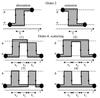 |
Fig. 1 Elementary processes and transition probabilities for the master equation developed at order-2 (upper part) and order-4 (lower part). At order-4, diagrams (1) and (2) are combinations of the order-2 elementary processes, whereas diagram (3) and (4) are not. |
The tranformation of the suite into the série is thus achieved by taking the contribution of each process in its native order, where it is “new”. Then, instead of considering all the processes of a given order and the suite of orders, this is replaced by the sum of the “new” contributions stemmed from all the lower orders. The problem then is to determine what are, for each order, the “new” and “non-new” contributions with respect to the lower orders. We found that the “non-new” contributions or processes may be identified by the following method. At a given order, we suspect some processes to be “non-new” and we write down the statistical equilibrium and radiative transfer equations considering only these processes of this order. The characteristics that are at the basis of the suspicion are described in Sect. 5.1 of Bommier (1997a). If we find that the statistical equilibrium and radiative transfer equation are unchanged with respect to their expression at the lower order, we conclude that there is nothing new there and that we successfully identified the “non-new” processes, which we can then eliminate in performing the transformation. We did that for order-4 with respect to order-2 (taking into account polarization), and then for order-6 (ignoring the polarization for simplicity, after we learned how to average it in order-4) with respect to order-4 and order-2. Indeed, some processes at order-6 are combinations of three order-2 processes, others are combinations of one order-4 and one order-2 process.
At order-4, a new term appeared in the emissivity, that we wrote under the form  (1)where ν is the outcoming photon frequency and Ω its propagation direction. We found that no additional term appeared in the emissivity at order-6. We tried some well-chosen order-8 contributions but all those and all the other “new” contributions of order-4 and order-6 to the radiative transfer or statistical equilibrium equations can be added to lower order contributions as a modification of their line profile. Another typical “new” term of this type is given by diagram (4) of Fig. 1. As a result, the general term of the profile series can then be written and the profile series may be added up, leading to a nonperturbative result. An initial profile of “nonzero” width had been first introduced and the addition yet broadens the profile. The initial width has to be discarded after the sum evaluation (see Sect. 3.4 below), which shows that the final result of overcoming the Markov approximation is twofold: first, the emissivity is comprised of the two contributions summarized in the above equation, and second, the line profile is properly included in the radiative transfer and statistical equilibrium equations.
The second term of the emissivity, ε(4)(ν,Ω), which originates from order-4, results from the diagram (3) of Fig. 1, where it is visible that there is a photon absorption, which takes place during τ3 + τ2, and a photon emission, which takes place during τ2 + τ1. Thus, there is a common time interval τ2, during which absorption and emission occur together, which permits a correlation between them such as the frequency coherence. It has to be noted that the absorption begins first. We show in Sect. 6.4 of Bommier (1997a) that in the case of an infinitely sharp lower level, and when the statistical equilibrium solution is reported in the emissivity to derive the redistribution functions, that the contribution of this order-4 term is of the form RII−RIII, and not only RII. In the atomic frame the redistribution functions are usually denoted as rII and rIII, whereas the notations RII and RIII are usually reserved for the laboratory frame redistribution functions. The rII redistribution function is the frequency-coherent redistribution function rII = δ(ν−ν′)φ(ν0−ν′), where ν and ν′ are respectively the outgoing and incoming photon frequencies, δ is the Dirac function, φ is the absorption line profile and ν0 the line center frequency, whereas rIII is the complete redistribution function rIII = φ(ν0−ν)φ(ν0−ν′). Therefore, it is yet the order-4 contribution that introduces scattering, and, in particular, frequency-coherent scattering or Rayleigh scattering. The lowest part of Fig. 1 shows that the upper level b is never “populated” during the process described by diagram (3) because the two transition amplitudes do not stay together in this level, contrary to the processes described by diagrams (1) and (2), where the upper level b is “populated” during τ2. Because level b is never populated during the Rayleigh scattering process, this naturally leads to the image of a “virtual” upper level in the Rayleigh scattering process. As the virtual level is infinitely sharp, this ensures the frequency coherence between incoming and outgoing frequencies in the Rayleigh scattering.
In the absence of collisions, the −rIII contribution originating from diagram (3) exactly compensates for that originating from diagrams (1) and (2) (or their order-2 equivalents), and as a result the scattering is entirely coherent in the far wings as well as in line center. However, absorption and emission are yet present in the statistical equilibrium equations and the upper level b is accordingly populated. rIII corresponds to the resonant scattering, which is described well by diagrams (1) and (2) of Fig. 1, and is comprised of absorption, which is followed by staying in the upper level and, in turn, followed by emission. At the line center, the virtual level joins the real level. Doppler broadening and transition to the laboratory frame should be considered also as described in Bommier (1997b), where, in the line center RII ≈ RIII, therefore, it is finally impossible to globally discriminate between coherent and incoherent scatterings in the line center. Our formalism is able to describe the full scattering, which we call Rayleigh/Raman scattering in the far wings (where the RIII contribution is negligible and where the scattering is then frequency coherent), and resonant scattering in the line centers.
Recently, Casini et al. (2014) presented a similar approach to describe the scattering. In a conference close to their paper publication (Meeting of the Working Group 2 of the COST Action MP 1104 “Polarization as a Tool to Study the Solar System and Beyond”, “Theory and Modeling of Polarization in Astrophysics”, Praha (Česká Republika), 5–8 May 2014), Casini reported that his theory was derived by developing the master equation at order-4 to repell the Markov approximation; however, he did not perform the above-described series transformation, in particular, to avoid having to discriminate between “new” and “non-new” contributions. He considered the whole order-4, but only this order. As we stated above, the Markov approximation is nevertheless required to close the equation, because it is not at infinite order. However, Bommier (1997a) had concluded that no new term in the emissivity appears at higher orders, only contributions to the line broadening. Therefore, in addition to his order-4 master equation, Casini introduced a line-broadening or “dressing the atom” formalism, which accounts for single photon absorption and emission. Thus, single photon absorption and emission are taken into account in the line broadening, but not as processes entering the statistical equilibrium equation. As for the atom “dressing”, we know this as the “dressed atom” approach the formalism describing an atom dressed by an intense laser field (Cohen-Tannoudji 1977; Cohen-Tannoudji & Reynaud 1977), whereas present astrophysical aplications are concerned with the limit of a weak radiation field (see next subsection).
The order-4 processes (in the case of a 2-level atom) are comprised neither of absorption nor emission, but of scattering, where emission and absorption are grouped in a single process (in the collisionless regime). The original, pure, order-4 statistical equilibrium equation results in being undetermined because the upper level can never be reached as the final state of a process starting from the lower level at least in the absence of collision, as we remarked above. Casini et al. (2014) concur at the end of their Sect. 2: “In the absence of collisions (i.e. at zero temperature), the process that populates the upper term by radiative absorption is inhibited in the limit of infinitely sharp lower levels”, so that “the upper levels can only be virtual”. In our approach, when we proceeded to the selection of the “non-new” contributions at order-4 with the method described above, the statistical equilibrium equation comprised of the “non-new” terms only was also undetermined, i.e., of the type 0 = 0, because the order-4 processes are all scattering (i.e., absorption and emission grouped in a single process), for the two-level (or two-term) atom. If we discard the vanishing coefficient on each side of the equation, however, we recover the lower order-2 equation, thus validating our selection of the “non-new” contributions. Thus, although “new” contributions are also found at order-4, we think that Casini et al. (2014) do not provide any statistical equilibrium equation because this results in being the undetermined type, at least in the absence of collisions because, as stated above, in the absence of collisions the upper level can never be reached as the final state of an order-4 process starting from the lower level.
If the development was made at order-6 instead, populating the upper level would be again possible because the elementary process, for instance, would be absorption that is followed by emission that is followed by absorption again, thus ending in the upper level. Statistical equilibrium equations would then be derived. The form of the statistical equilibrium equations would be the usual one, except for the order-6 line profile shapes. We generalize this discussion in Sect. 4.4 below.
We also state above that, at order-4, the initial conditions are explicitly included in the master equation. This is a difficulty, which we also resolved via our series transformation described above, because at the lowest order, order-2, this is not the case, and when this order is kept in the development, this avoids a difficulty with the initial conditions. Although Casini et al. (2014) state, in their Sect. 2, that the “initial conditions for the system’s density matrix are handled in a similar way” (similar to our method), this cannot be the case because our handling is a consequence of the series transformation we performed, which Casini et al. (2014) on the contrary, avoided carrying out.
It is important not to mix the two formalisms. It would be strongly inconsistent to envisage complementing the radiative transfer equation given by Casini et al. (2014) with our statistical equilibrium equation because Casini et al. (2014) did not provide this equation. Although their emissivity also includes two contributions as ours, the respective contributions are individually different from ours. The final result in terms of redistribution function is however in agreement with our results of Bommier (1997a,b). All occurs as if the statistical equilibrium, which is avoided in their order-4 approach, is at least already partly resolved (for a two-level or two-term atom) inside the radiative transfer equation itself, leading to different coefficients, but agreement on the final combined solution in terms of redistribution function.
2.2. The multiphoton Raman scattering
In order to generalize our formalism of Bommier (1997a,b) to a multilevel-multiline atom, we have to examine how the different terms represented in Fig. 1 have to be generalized. Single photon absorption or emission are unchanged and may occur between any levels provided that the line connecting them is permitted. Diagrams (1) and (2) are both simply a series of such single photon processes. Diagram (3) obviously generalizes into Raman scattering with final level c that is different from the initial level a.
In the general case, however, higher order Raman scattering is to be envisaged, involving several upper levels b,d,e,f... with associated or combined absorption and emission in intermediate lines. We denote such a general process as the “multiphoton Raman scattering”. In addition to this general process, multiphoton absorption or emission could also occur in a multilevel atom. However, we point out that it is well known that the transition probabilities associated with such multiphoton processes behave like powers of the average photon number per mode  (Grynberg & Cagnac 1977), and, as we discussed at the beginning of Sect. 2 of Bommier (1997a), visible lines at the surface of the Sun range in the weak radiation field regime with
  . Indeed, at the surface of the sun one has
  (2)where Trad is the incident radiation temperature, about 6000 K, and at λ = 600 nm. The condition may not be satisfied for some infrared and far-infrared lines, which may be also emitted by a multilevel atom, even if the condition is fulfilled for the lines of interest. Our formalism does presently not include terms in powers of . This will be the object of future investigations.
As a consequence, we presently consider multiphoton processes as negligible for our astrophysical purposes and, in this case, the generalization of our formalism only requires the generalization of the Rayleigh scattering term into the Raman scattering (with different initial and final levels), and the accounting for all the processes that able to reach or leave any level, upper or lower similarly. This is described in the next section. We also take induced emission into account.
3. Equations for the multilevel-multiline atom
3.1. Taking the Doppler redistribution into account
The quantum description of atom and radiation used here has to be complemented by a quantum description for the Doppler effect. Though the well-known frequency Doppler shift can also be derived in a quantum formulation using energy and momentum conservation (see for instance Louisell 1973; Loudon 1973), the Doppler effect has been introduced in the statistical equilibrium equation derivation based on quantum electrodynamics by Sahal-Brechot et al. (1998). We use the same notations as in the Sahal-Brechot et al. (1998) paper.
We denote with p the atomic momentum operator. p = mv in the non-relativistic limit, where m is the atomic mass and v is the atomic velocity.
The eigenstates of the translation Hamiltonian (to be added to the rest-frame atomic Hamiltonian)  (3)are the plane waves |p⟩. The eigenstates of the atomic Hamiltonian in the laboratory frame then take the form
  (4)where αJM are the quantum numbers characterizing the internal state ( α representing a group of numbers), whereas p characterizes the external state. For the atom, the atomic velocity is an external freedom degree. The elements of the atomic density matrix σ are of the form
  (5)If it is assumed that the atomic velocity does not change during the scattering process (see the discussion in Sect. 2.2 of Sahal-Brechot et al. 1998, and the discussion in the following Sect. 4.1) , the atomic velocity is conserved, and the total Hamiltonian is diagonal in |p⟩. Physically, this corresponds to the assumption that the time between two velocity-changing collisions is very long with respect to the level radiative lifetimes. Owing to the relative mass effect, only elastic collisions with particles with about same masses or higher masses than the radiating atom have to be considered. Under solar conditions, such collisional rates are very weak with respect to the radiative rates. Therefore, those terms of the atomic density matrix with p ≠ p′ are completely decoupled from those terms that have p = p′. We can thus define a reduced density matrix σ(v,t) through the equation
  (6)The diagonal element ⟨αJM|σ(v,t)|αJM⟩ is the joint probability of finding an atom with velocity v in the level αJM.
Following Sahal-Brechot et al. (1998), the Doppler effect is taken into account by replacing any angular frequency ω that appears in the line profiles by ω−k·v, where k is the radiation wavevector. In terms of frequencies, a frequency ν of a line profile has to be replaced by the Doppler shifted frequency 
 (7)where Ω denotes the radiation propagation direction.
In the following, we skip to the normalized density matrix ρ(v,t) defined by 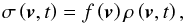 (8)where
  is the normalized atomic velocity distribution function (which is independent of the internal state of the atom).
In addition, we assume in the following that there is no coupling between the reduced density matrices σ(v,t) and σ(v′,t) relative to different velocities v and v′. The effect of velocity changing by collision is ignored or is assumed to be negligible (see the discussion below in Sect. 4). The statistical equilibrium equations introduced below have to be resolved for each velocity class.
3.2. Statistical equilibrium equations
We present below the generalization of the equations of Bommier (1997a,b) to the multilevel atom. These equations are derived from the formalism described above and are at the basis of the new code XTAT that we are developing for non-LTE polarized line formation with redistribution, and will be described in the next paper of this series (Bommier 2016). As in Bommier (1980), the statistical equilibrium equations for the multilevel atomic density matrix ρ are given by ![\begin{eqnarray} \dfrac{\mathrm{d}}{\mathrm{d}t}\ ^{\alpha _{1}J_{1}J_{1}^{\prime }}\rho _{M_{1}M_{1}^{\prime }}\left( \vec{r},\vec{v}\right) &= & -\dfrac{\mathrm{i}}{\hbar }\left[E\left( \alpha _{1}J_{1}M_{1}\right) -E\left( \alpha _{1}J_{1}^{\prime }M_{1}^{\prime }\right) \right] \ \nonumber\\[2mm] && \quad \times\, ^{\alpha _{1}J_{1}J_{1}^{\prime }}\rho _{M_{1}M_{1}^{\prime }}\left( \vec{r},\vec{v}\right) \nonumber\\[2mm] && \quad +\dsum\limits_{\alpha _{2}J_{2}J_{2}^{\prime }M_{2}M_{2}^{\prime }}\Gamma _{\alpha _{1}J_{1}J_{1}^{\prime }M_{1}M_{1}^{\prime }\leftarrow \alpha _{2}J_{2}J_{2}^{\prime }M_{2}M_{2}^{\prime }}\ \nonumber\\[2mm] && \quad \times\, ^{\alpha _{2}J_{2}J_{2}^{\prime }}\rho _{M_{2}M_{2}^{\prime }}\left( \vec{r},\vec{v}\right) \nonumber\\[2mm] && \quad -\dfrac{1}{2}\!\dsum\limits_{J"_{1}M"_{1}}\left\{ \dsum\limits_{\alpha _{2}J_{2}M_{2}}\Gamma _{\alpha _{2}J_{2}J_{2}M_{2}M_{2}\leftarrow \alpha _{1}J"_{1}J_{1}M"_{1}M_{1}}\ \right. \nonumber\\[2mm] && \quad \times\, ^{\alpha _{1}J"_{1}J_{1}^{\prime }}\rho _{M"_{1}M_{1}^{\prime }}\left( \vec{r},\vec{v}\right) \nonumber\\[2mm] && \quad +\dsum\limits_{\alpha _{2}J_{2}M_{2}}\Gamma _{\alpha _{2}J_{2}J_{2}M_{2}M_{2}\leftarrow \alpha _{1}J_{1}^{\prime }J"_{1}M_{1}^{\prime }M"_{1}} \nonumber\\[2mm] && \quad \times \left. ^{\alpha _{1}J_{1}J"_{1}}\rho _{M_{1}M"_{1}}\left( \vec{r},\vec{v}\right)\hspace*{-0.8cm}\phantom{\dsum\limits_{\alpha _{2}J_{2}M_{2}}} \right\} . \label{EqStat} \end{eqnarray}](/articles/aa/full_html/2016/07/aa26798-15/aa26798-15-eq67.png) (9)The energy difference accounts for Zeeman splitting, fine and hyperfine splittings (replacing L,S,J by J,I,F), and eventually incomplete Paschen-Back effect. In this last case, J is no longer a “good quantum number”, and there is no symmetry in the density matrix elements, so that there is no advantage to applying the irreducible tensor formalism because the number of nonzero elements is not reduced and the formalism is more complex. Therefore we preferred to apply the dyadic formalism. Here, the transition coefficients Γ have new expressions that include the line profile. The expression of these coefficients is different for spontaneous emission, induced emission and absorption. Introducing
(9)The energy difference accounts for Zeeman splitting, fine and hyperfine splittings (replacing L,S,J by J,I,F), and eventually incomplete Paschen-Back effect. In this last case, J is no longer a “good quantum number”, and there is no symmetry in the density matrix elements, so that there is no advantage to applying the irreducible tensor formalism because the number of nonzero elements is not reduced and the formalism is more complex. Therefore we preferred to apply the dyadic formalism. Here, the transition coefficients Γ have new expressions that include the line profile. The expression of these coefficients is different for spontaneous emission, induced emission and absorption. Introducing ![\begin{eqnarray} && X\left( \alpha _{2}J_{2}J_{2}^{\prime }\rightarrow \alpha _{1}J_{1}J_{1}^{\prime }\right) =\left( -1\right) ^{J_{1}^{\prime }-J_{1}+J_{2}^{\prime }-J_{2}} \nonumber\\[2mm] && \times \left[\left( 2J_{1}+1\right) \left( 2J_{2}+1\right) \left( 2J_{1}^{\prime }+1\right) \left( 2J_{2}^{\prime }+1\right) \right] ^{1/2} \nonumber\\[2mm] && \times \begin{Bmatrix} J_{1} & 1 & J_{2} \\ L_{2} & S & L_{1} \end{Bmatrix} \begin{Bmatrix} J_{1}^{\prime } & 1 & J_{2}^{\prime } \\ L_{2} & S & L_{1} \end{Bmatrix} \left( 2L_{2}+1\right), \end{eqnarray}](/articles/aa/full_html/2016/07/aa26798-15/aa26798-15-eq72.png) (10)the transition coefficients Γ can be expressed as follows. The collision effects may be added in these equations following the formalism developed in Bommier & Sahal-Bréchot (1991) for the inelastic collisions and in Kerkeni & Bommier (2002) for the elastic collisions, and reported below in Sect. 3.5. One has
(10)the transition coefficients Γ can be expressed as follows. The collision effects may be added in these equations following the formalism developed in Bommier & Sahal-Bréchot (1991) for the inelastic collisions and in Kerkeni & Bommier (2002) for the elastic collisions, and reported below in Sect. 3.5. One has


![\begin{eqnarray} \Gamma _{\alpha _{1}J_{1}J_{1}^{\prime }M_{1}M_{1}^{\prime }\leftarrow \alpha _{2}J_{2}J_{2}^{\prime }M_{2}M_{2}^{\prime }}^{\mathrm{sp} }&=& X\left( \alpha _{2}J_{2}J_{2}^{\prime }\rightarrow \alpha _{1}J_{1}J_{1}^{\prime }\right) \left( -1\right) ^{M_{1}-M_{1}^{\prime }} \nonumber\\[2mm] && \quad\times A\left( \alpha _{2}L_{2}S\rightarrow \alpha _{1}L_{1}S\right) \nonumber\\[2mm] &&\quad \times \left( \begin{array}{ccc} J_{1} & 1 & J_{2} \\ -M_{1} & -p & M_{2} \end{array} \right) \nonumber\\[2mm] &&\quad \times \left( \begin{array}{ccc} J_{1}^{\prime } & 1 & J_{2}^{\prime } \\ -M_{1}^{\prime } & -p & M_{2}^{\prime } \end{array} \right) , \label{spontaneous} \end{eqnarray}](/articles/aa/full_html/2016/07/aa26798-15/aa26798-15-eq75.png)
![\begin{eqnarray} \Gamma _{\alpha _{1}J_{1}J_{1}^{\prime }M_{1}M_{1}^{\prime }\leftarrow \alpha _{2}J_{2}J_{2}^{\prime }M_{2}M_{2}^{\prime }}^{\mathrm{ind }}&=& X\left( \alpha _{2}J_{2}J_{2}^{\prime }\rightarrow \alpha _{1}J_{1}J_{1}^{\prime }\right) \nonumber\\[2mm] && \quad\times 3B\left( \alpha _{2}L_{2}S\rightarrow \alpha _{1}L_{1}S\right) \nonumber\\[2mm] && \quad\times \dint \mathrm{d}\nu \doint \dfrac{\mathrm{d}\vec{\Omega}}{ 4\pi }\left( -1\right) ^{M_{1}-M_{1}^{\prime }}J_{-p-p^{\prime }}\left( \tilde{\nu}\right) \nonumber\\[2mm] && \quad\times \left( \! \! \begin{array}{ccc} J_{1} & 1 & J_{2} \\ -M_{1} & -p^{\prime } & M_{2} \end{array} \! \!\right) \nonumber\\[2mm] && \quad\times \left( \! \! \begin{array}{ccc} J_{1}^{\prime } & 1 & J_{2}^{\prime } \\ -M_{1}^{\prime } & -p & M_{2}^{\prime } \end{array} \! \!\right) \nonumber\\[2mm] && \quad\times \left[\dfrac{1}{2}\Phi _{ba}^{\ast }\left( \nu _{\alpha _{2}J_{2}^{\prime }M_{2}^{\prime },\alpha _{1}J_{1}^{\prime }M_{1}^{\prime }}-\tilde{\nu}\right) \right. \nonumber\\ && \quad+\left. \dfrac{1}{2}\Phi _{ba}\left( \nu _{\alpha _{2}J_{2}M_{2},\alpha _{1}J_{1}M_{1}}-\tilde{\nu}\right) \right] , \end{eqnarray}](/articles/aa/full_html/2016/07/aa26798-15/aa26798-15-eq76.png)
![\begin{eqnarray} \Gamma _{\alpha _{1}J_{1}J_{1}^{\prime }M_{1}M_{1}^{\prime }\leftarrow \alpha _{2}J_{2}J_{2}^{\prime }M_{2}M_{2}^{\prime }}^{\mathrm{abs }}\!&=& X\left( \alpha _{2}J_{2}J_{2}^{\prime }\rightarrow \alpha _{1}J_{1}J_{1}^{\prime }\right) \nonumber\\ &&\quad \times 3B\left( \alpha _{2}L_{2}S\rightarrow \alpha _{1}L_{1}S\right) \nonumber\\ &&\quad \times\!\! \!\dint\!\! \mathrm{d}\nu \!\doint\! \dfrac{\mathrm{d}\vec{\Omega}}{ 4\pi }\!\left( -1\right) ^{M_{1}-M_{1}^{\prime }+p+p^{\prime }}\!\!J_{-p-p^{\prime }}\left( \tilde{\nu}\right) \nonumber\\ &&\quad \times \left( \! \! \begin{array}{ccc} J_{1} & 1 & J_{2} \\ -M_{1} & p & M_{2} \end{array} \! \!\right) \nonumber\\ &&\quad \times \left( \! \! \begin{array}{ccc} J_{1}^{\prime } & 1 & J_{2}^{\prime } \\ -M_{1}^{\prime } & p^{\prime } & M_{2}^{\prime } \end{array} \! \!\right) \nonumber\\ && \quad\times \left[\dfrac{1}{2}\Phi _{ba}\left( \nu _{\alpha _{1}J_{1}^{\prime }M_{1}^{\prime },\alpha _{2}J_{2}^{\prime }M_{2}^{\prime }}-\tilde{\nu}\right) \right. \nonumber\\ && \quad+\left. \dfrac{1}{2}\Phi _{ba}^{\ast }\left( \nu _{\alpha _{1}J_{1}M_{1},\alpha _{2}J_{2}M_{2}}-\tilde{\nu}\right) \right] , \end{eqnarray}](/articles/aa/full_html/2016/07/aa26798-15/aa26798-15-eq77.png)
In principle, there are also imaginary contributions to the statistical equilibrium equations, comprised of level shift terms, as shown in Eqs. (34)–(35) of Bommier & Sahal-Brechot (1978). The δ (Dirac delta) and P (Cauchy principal value) functions of these equations, issued from an order-2 development, have to be replaced by the real and imaginary part of the complex Lorentz profile of Eq. (22) below. The real part is an absorption profile and the imaginary part is a dispersion profile. For the practical applications we considered, all within the weak radiation field limit, we estimated that the level shift effect due to the atom-photon interaction is very small with respect to all the frequencies at play, which is also the case for all the Zeeman sublevels and, thereby, we have ignored this effect.
3.3. Radiative transfer equation
It is well known (see for instance Landi Degl’Innocenti & Landolfi 2004, p. 350) that the polarized radiative transfer equation takes the form 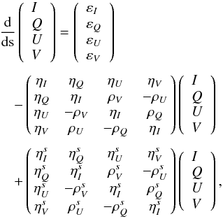 (14)where (I,Q,U,V) are the Stokes parameters, which may alternatively be referred to by the four indices
  , respectively. The εs are the emissivities and the ηs the absorption coefficients (ρs for the magneto-optical effects), and the upper s index stands for “stimulated emission”. These coefficients are related to the atomic density matrix elements. Following the method developed in Bommier (1997a,b), these coefficients for the multilevel-multiline atom are as follows:
-
for emission, the emissivity is the sum of thespontaneous emission contribution denoted asε(2), issued from order-2, and of a Rayleigh (or Raman) scattering term denoted as ε(4), issued from order-4. For order-2, one has
![\begin{eqnarray} \varepsilon _{i}^{\left( 2\right) }\left( \vec{r},\nu ,\vec{\Omega} \right) &=&\dfrac{h\nu }{4\pi }\mathcal{N} \times \dsum\limits_{\alpha _{1}J_{1}J_{1}^{\prime }M_{1}M_{1}^{\prime }\alpha _{2}J_{2}M_{2}} \nonumber\\ &&\quad\times \dint \mathrm{d}^{3}\vec{v}f\left( \vec{v}\right) \ ^{\alpha _{1}J_{1}J_{1}^{\prime }}\rho _{M_{1}M_{1}^{\prime }}\left( \vec{r},\vec{v} \right) \nonumber\\ && \quad\times \mathcal{T}_{-p-p^{\prime }}\left( i,\vec{\Omega}\right) 3A\left( \alpha _{1}L_{1}S\rightarrow \alpha _{2}L_{2}S\right) \nonumber\\ &&\quad \times X\left( \alpha _{1}J_{1}J_{1}^{\prime }\rightarrow \alpha _{2}J_{2}J_{2}\right) \nonumber\\ && \quad\times \left( \! \! \begin{array}{ccc} J_{2} & 1 & J_{1} \\ -M_{2} & -p^{\prime } & M_{1} \end{array} \! \!\right) \left(\! \! \begin{array}{ccc} J_{2} & 1 & J_{1}^{\prime } \\ -M_{2} & -p & M_{1}^{\prime } \end{array} \! \!\right) \nonumber\\ && \quad\times \left[\dfrac{1}{2}\Phi _{ba}\left( \nu _{\alpha _{1}J_{1}^{\prime }M_{1}^{\prime },\alpha _{2}J_{2}M_{2}}-\tilde{\nu}\right) \right. \nonumber\\ && \quad+\left. \dfrac{1}{2}\Phi _{ba}^{\ast }\left( \nu _{\alpha _{1}J_{1}M_{1},\alpha _{2}J_{2}M_{2}}-\tilde{\nu}\right) \right] , \end{eqnarray}](/articles/aa/full_html/2016/07/aa26798-15/aa26798-15-eq87.png) (15)where
(15)where  is the atom density. In the derivation of Bommier (1997a), which is 2-level, the order-4 term describes the Rayleigh scattering, a process starting from the lower level a, passing by the upper b level but not really populating it, and returning to the lower level a. Here we are interested in multilevel atom. In addition to Rayleigh scattering, Raman scattering may occur. The Raman scattering process starts from an initial level a or J1M1 (or eventually from a coherence between J1M1 and
  ), passes by an upper b level denoted as J2M2 or
  (they may be different because they correspond to two different scattering amplitudes, as already stated), and returns to a third level c denoted as J3M3 (only one level for closure). The expression of
  given below fully accounts for this Raman scattering, which is a generalization of Rayleigh scattering. Rigorously, other new terms in the emissivity appear at higher orders of the development, involving more than three levels, such as absorption from a to b, emission from b to c ≠ a, reabsorption from c to d ≠ b, and re-emission from d to e ≠ a,c, where all these processes are correlated. However, all these new terms would involve more than one scattered photon. These terms would correspond to multiphoton Rayleigh/Raman processes, which are not well known, and are very probably negligible in weak radiation fields. We neglect terms of this type and we then get for the second emissivity contribution
 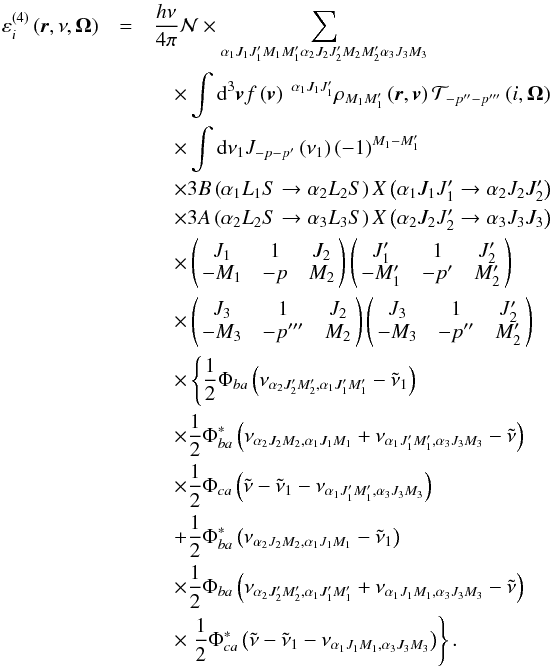 (16)When the a and c levels belong to the ground level of the atom, the width of Φca is zero (neglecting the broadening by radiative absorption) and Φca may be replaced by the δ Dirac function, which makes the frequency conservation appear in a more clear manner.
 -
for absorption, one has for the absorption coefficients
![\begin{eqnarray} \eta _{i}\left( \vec{r},\nu ,\vec{\Omega}\right) &=&\dfrac{h\nu }{ 4\pi }\mathcal{N} \times \dsum\limits_{\alpha _{1}J_{1}J_{1}^{\prime }M_{1}M_{1}^{\prime }\alpha _{2}J_{2}M_{2}}\nonumber\\ &&\quad \times \dint \mathrm{d}^{3}\vec{v}f\left( \vec{v}\right) \ ^{\alpha _{1}J_{1}J_{1}^{\prime }}\rho _{M_{1}M_{1}^{\prime }}\left( \vec{r},\vec{v} \right)\nonumber\\ &&\quad \times \mathcal{T}_{-p-p^{\prime }}\left( i,\vec{\Omega}\right) \left( -1\right) ^{M_{1}-M_{1}^{\prime }} 3B\left( \alpha _{1}L_{1}S\!\rightarrow\! \alpha _{2}L_{2}S\right)\nonumber\\ &&\quad \times X\left( \alpha _{1}J_{1}J_{1}^{\prime }\rightarrow \alpha _{2}J_{2}J_{2}\right)\nonumber\\ &&\quad \times \left(\! \! \begin{array}{ccc} J_{1} & 1 & J_{2} \\ -M_{1} & -p & M_{2} \end{array} \! \!\right) \left( \! \! \begin{array}{ccc} J_{1}^{\prime } & 1 & J_{2} \\ -M_{1}^{\prime } & -p^{\prime } & M_{2} \end{array} \! \!\right)\nonumber\\ &&\quad \times \left[\dfrac{1}{2}\Phi _{ba}\left( \nu _{\alpha _{2}J_{2}M_{2},\alpha _{1}J_{1}M_{1}}-\tilde{\nu}\right) \right.\nonumber\\ &&\quad +\left. \dfrac{1}{2}\Phi _{ba}^{\ast }\left( \nu _{\alpha _{2}J_{2}M_{2},\alpha _{1}J_{1}^{\prime }M_{1}^{\prime }}-\tilde{\nu}\right) \right] , \end{eqnarray}](/articles/aa/full_html/2016/07/aa26798-15/aa26798-15-eq102.png) (17)and one has for the magneto-optical effects
(17)and one has for the magneto-optical effects ![\begin{eqnarray} \rho _{i}\left( \vec{r},\nu ,\vec{\Omega}\right) &=&\dfrac{h\nu }{ 4\pi }\mathcal{N} \times \dsum\limits_{\alpha _{1}J_{1}J_{1}^{\prime }M_{1}M_{1}^{\prime }\alpha _{2}J_{2}M_{2}}\nonumber\\ &&\quad\times\dint \mathrm{d}^{3}\vec{v}f\left( \vec{v}\right) \ ^{\alpha _{1}J_{1}J_{1}^{\prime }}\rho _{M_{1}M_{1}^{\prime }}\left( \vec{r},\vec{v} \right)\nonumber\\ &&\quad \times \mathcal{T}_{-p-p^{\prime }}\left( i,\vec{\Omega}\right) \left( -1\right) ^{M_{1}-M_{1}^{\prime }}\nonumber\\ &&\quad \times 3B\left( \alpha _{1}L_{1}S\rightarrow \alpha _{2}L_{2}S\right)\nonumber\\ &&\quad \times X\left( \alpha _{1}J_{1}J_{1}^{\prime }\rightarrow \alpha _{2}J_{2}J_{2}\right)\nonumber\\ &&\quad \times \left(\! \! \begin{array}{ccc} J_{1} & 1 & J_{2} \\ -M_{1} & -p & M_{2} \end{array} \! \!\right)\nonumber\\ &&\quad \times \left( \! \! \begin{array}{ccc} J_{1}^{\prime } & 1 & J_{2} \\ -M_{1}^{\prime } & -p^{\prime } & M_{2} \! \!\end{array} \right)\nonumber\\ &&\quad \times \left( -\mathrm{i}\right) \left[\dfrac{1}{2}\Phi _{ba}\left( \nu _{\alpha _{2}J_{2}M_{2},\alpha _{1}J_{1}M_{1}}-\tilde{\nu} \right) \right.\nonumber\\ &&\quad -\left. \dfrac{1}{2}\Phi _{ba}^{\ast }\left( \nu _{\alpha _{2}J_{2}M_{2},\alpha _{1}J_{1}^{\prime }M_{1}^{\prime }}-\tilde{\nu}\right) \right] . \end{eqnarray}](/articles/aa/full_html/2016/07/aa26798-15/aa26798-15-eq103.png) (18)
(18) -
for stimulated emission, one has for the emission coefficients
![\begin{eqnarray} \eta _{i}^{s}\left( \vec{r},\nu ,\vec{\Omega}\right) &=&\dfrac{h\nu }{ 4\pi }\mathcal{N} \dsum\limits_{\alpha _{1}J_{1}J_{1}^{\prime }M_{1}M_{1}^{\prime }\alpha _{2}J_{2}M_{2}} \nonumber\\ &&\quad \times\dint \mathrm{d}^{3}\vec{v}f\left( \vec{v}\right) \ ^{\alpha _{1}J_{1}J_{1}^{\prime }}\rho _{M_{1}M_{1}^{\prime }}\left( \vec{r},\vec{v} \right) \nonumber\\ &&\quad \times \mathcal{T}_{-p-p^{\prime }}\left( i,\vec{\Omega}\right) \nonumber\\ &&\quad \times 3B\left( \alpha _{1}L_{1}S\rightarrow \alpha _{2}L_{2}S\right) \nonumber\\ &&\quad \times X\left( \alpha _{1}J_{1}J_{1}^{\prime }\rightarrow \alpha _{2}J_{2}J_{2}\right) \nonumber\\ &&\quad \times \left( \! \! \begin{array}{ccc} J_{1} & 1 & J_{2} \\ -M_{1} & p^{\prime } & M_{2} \end{array} \! \!\right) \nonumber\\ &&\quad \times \left( \! \! \begin{array}{ccc} J_{1}^{\prime } & 1 & J_{2} \\ -M_{1}^{\prime } & p & M_{2} \end{array} \! \!\right) \nonumber\\ &&\quad \times \left[\dfrac{1}{2}\Phi _{ba}\left( \nu _{\alpha _{1}J_{1}^{\prime }M_{1}^{\prime },\alpha _{2}J_{2}M_{2}}-\tilde{\nu}\right) \right. \nonumber\\ &&\quad +\left. \dfrac{1}{2}\Phi _{ba}^{\ast }\left( \nu _{\alpha _{1}J_{1}M_{1},\alpha _{2}J_{2}M_{2}}-\tilde{\nu}\right) \right] , \end{eqnarray}](/articles/aa/full_html/2016/07/aa26798-15/aa26798-15-eq104.png) (19)and for the magneto-optical effects
(19)and for the magneto-optical effects ![\begin{eqnarray} \rho _{i}^{s}\left( \vec{r},\nu ,\vec{\Omega}\right) &=&\dfrac{h\nu }{ 4\pi }\mathcal{N} \dsum\limits_{\alpha _{1}J_{1}J_{1}^{\prime }M_{1}M_{1}^{\prime }\alpha _{2}J_{2}M_{2}} \nonumber\\ &&\quad \times \dint \mathrm{d}^{3}\vec{v}f\left( \vec{v}\right) \ ^{\alpha _{1}J_{1}J_{1}^{\prime }}\rho _{M_{1}M_{1}^{\prime }}\left( \vec{r},\vec{v} \right) \nonumber\\ &&\quad \times \mathcal{T}_{-p-p^{\prime }}\left( i,\vec{\Omega}\right) \nonumber\\ &&\quad \times 3B\left( \alpha _{1}L_{1}S\rightarrow \alpha _{2}L_{2}S\right) \nonumber\\ &&\quad \times X\left( \alpha _{1}J_{1}J_{1}^{\prime }\rightarrow \alpha _{2}J_{2}J_{2}\right) \nonumber\\ &&\quad \times \left( \! \! \begin{array}{ccc} J_{1} & 1 & J_{2} \\ -M_{1} & p^{\prime } & M_{2} \end{array} \! \!\right) \nonumber\\ &&\quad \times \left( \! \! \begin{array}{ccc} J_{1}^{\prime } & 1 & J_{2} \\ -M_{1}^{\prime } & p & M_{2} \end{array} \! \!\right) \nonumber\\ &&\quad \times \left( -\mathrm{i}\right) \left[\dfrac{1}{2}\Phi _{ba}\left( \nu _{\alpha _{1}J_{1}^{\prime }M_{1}^{\prime },\alpha _{2}J_{2}M_{2}}-\tilde{\nu}\right) \right. \nonumber\\ &&\quad -\left. \dfrac{1}{2}\Phi _{ba}^{\ast }\left( \nu _{\alpha _{1}J_{1}M_{1},\alpha _{2}J_{2}M_{2}}-\tilde{\nu}\right) \right] . \end{eqnarray}](/articles/aa/full_html/2016/07/aa26798-15/aa26798-15-eq105.png) (20)
(20)
 , defined by Landi Degl’Innocenti & Landolfi (2004, p. 207)
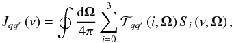 (21)where Si (i = 0,1,2,3) is one of the Stokes parameters, and Tqq′(i,Ω) is the spherical tensor for polarimetry defined and tabulated by Landi Degl’Innocenti & Landolfi (2004, Table 5.3 p. 206), which depends on the Stokes index i and on the direction of the incident radiation referred to by Ω.
3.4. Line profiles
The profile Φba is defined as in Eq. (63) of Bommier (1997a) (22)where ω = 2πν is the angular frequency, and γba and Δba are the width and shift coefficients defined Eqs. (16)–(19) of Omont et al. (1972). Subscripts a and b may correspond as well to two levels (α1L1S) and (α2L2S) connected by a permitted radiative transition, as to two levels that are not connected, such as the levels a (initial) and c (final) of the Raman scattering contribution to the emissivity, in Eq. (16) above. Rayleigh scattering is a particular case of the Raman scattering by considering a = c. Following Omont et al. (1972), in both cases of permitted or forbidden radiative transitions, one has
  (23)where 1/Γa (resp. 1/Γb) is the natural lifetime of level a (resp. b), and
  (24)is the collisional contribution (broadening and shift) averaged over the perturbers and S is the collision S-matrix of the individual collision (impact approximation), following Eq. (71) of Baranger (1958). When a = c , one has obviously
  (25)where
  (26)We define the elementary profile central frequency να2J2M2,α1J1M1 as
 ![\begin{equation} \nu _{\alpha _{2}J_{2}M_{2},\alpha _{1}J_{1}M_{1}}=\frac{1}{h}\left[E\left( \alpha _{2}J_{2}M_{2}\right) -E\left( \alpha _{1}J_{1}M_{1}\right) \right] \ . \end{equation}](/articles/aa/full_html/2016/07/aa26798-15/aa26798-15-eq127.png) (27)When a magnetic field is present, the Zeeman energy shift has to be taken into account here.
(27)When a magnetic field is present, the Zeeman energy shift has to be taken into account here.
In our development, each Zeeman component profile is centered at the exact frequency or wavelength of the component. A priori, the width could also depend on the Zeeman component. However, as described in Sect. 5.2 of Bommier (1997a), diagrams such as (4) of Fig. 1 are responsible for additional contributions to the profile that modify it. The series of modifications can be added up and broaden the profile. This series is proportional to the multiplet spontaneous emission probability because the dependence on the other quantum numbers (in particular the magnetic quantum numbers) is the same for the whole series so that it can be factorized, leading to the coefficients given above in Sect. 3. As a result of the sum, the profile is broadened by this multiplet spontaneous emission probability, which is independent of the magnetic quantum number. Besides, the profile is a consequence of the evolution operators, which take all of the other possible interactions into account during one atom-photon interaction, whereas our development also takes multiple atom-photon interactions into account by considering the higher orders.Thus these multiple atom-photon interactions are then counted twice, so that for the line broadening only one emission probability has to be finally retained instead of two. A more detailed discussion of this double counting can be found in Sect. 5.3, Eq. (83) of Bommier (1997a).
However, the atom also interacts with other systems, such as perturbers. These interactions are also responsible for line broadening. In principle, one should consider a development that mixes the different interactions, but this is carried out by the Baranger (1958) formalism as introduced by Omont et al. (1972) in the evolution operators. These results are described here.
Our development has shown that the radiative broadening of all the Zeeman components is the same. Similarly, in most cases the magnetic field effect is negligible during the collisions responsible for the collisional line broadening. This requires a small collision time with respect to the inverse Larmor frequency. Similarly, the hyperfine structure and even the fine structure can generally be neglected during the collision, at least in solar conditions. The fine or hyperfine components of a spectral line each accordingly have the same width and shift. The component collisional width and shift can be written as found in Sahal-Bréchot & Bommier (2014), ![\begin{eqnarray} \gamma _{ba}^{(c)}+\mathrm{i}\Delta _{ba} &=&N_{\mathrm{P} }\int_{0}^{\infty }vf(v)\mathrm{d}v\ \int_{0}^{\infty }2\pi \rho \mathrm{d}\rho\notag \\[-1.5mm] &&\quad\times \left[1-\sum_{M_{i}M_{i}^{\prime }M_{f}M_{f}^{\prime }\mu }(-1)^{2J_{f}+M_{f}+M_{f}^{\prime }}\right. \notag \\[-1.5mm] &&\quad\times \begin{pmatrix} J_{i} & 1 & J_{f} \\ -M_{i} & \mu & M_{f} \end{pmatrix} \begin{pmatrix} J_{i} & 1 & J_{f} \\ -M_{i}^{\prime } & \mu & M_{f}^{\prime } \end{pmatrix} \notag \\[-1.5mm] &&\quad\times \left\langle \alpha _{f}J_{f}M_{f}\right\vert S\left\vert \alpha _{f}J_{f}M_{f}^{\prime }\right\rangle ^{\ast } \left. \left\langle \alpha _{i}J_{i}M_{i}\right\vert S\left\vert \alpha _{i}J_{i}M_{i}^{\prime }\right\rangle \phantom{\sum_{M_{i}M_{i}^{\prime }M_{f}M_{f}^{\prime }\mu }}\hspace*{-1.4cm}\right] , \end{eqnarray}](/articles/aa/full_html/2016/07/aa26798-15/aa26798-15-eq128.png) (28)where NP is the perturber density, v the perturber velocity and ρ the perturber impact parameter. Considering the transition matrix T = 1−S, and given the unitarity of the S matrix SS† = 1, which leads to T + T† = TT†, for the width (double width) one has
(28)where NP is the perturber density, v the perturber velocity and ρ the perturber impact parameter. Considering the transition matrix T = 1−S, and given the unitarity of the S matrix SS† = 1, which leads to T + T† = TT†, for the width (double width) one has ![\begin{eqnarray} 2\gamma _{ba}^{(c)} &=&N_{\mathrm{P}}\int_{0}^{\infty }vf(v) \mathrm{d}v \label{interference}\notag \\ &&\quad\times \Bigg[\sum_{\alpha J}\sigma (\alpha _{i}J_{i}\rightarrow \alpha J)+\sum_{\alpha ^{\prime }J^{\prime }}\sigma (\alpha _{f}J_{f}\rightarrow \alpha ^{\prime }J^{\prime }) \notag \\ &&\quad-2\func{Re}\int_{0}^{\infty }2\pi \rho \mathrm{d}\rho \sum_{M_{i}M_{i}^{\prime }M_{f}M_{f}^{\prime }\mu }(-1)^{2J_{f}+M_{f}+M_{f}^{\prime }} \notag \\ &&\quad\times \begin{pmatrix} J_{i} & 1 & J_{f} \\ -M_{i} & \mu & M_{f} \end{pmatrix} \begin{pmatrix} J_{i} & 1 & J_{f} \\ -M_{i}^{\prime } & \mu & M_{f}^{\prime } \end{pmatrix} \notag \\ &&\quad\times \left\langle \alpha _{f}J_{f}M_{f}\right\vert T\left\vert \alpha _{f}J_{f}M_{f}^{\prime }\right\rangle ^{\ast } \notag \\ &&\quad\times \left\langle \alpha _{i}J_{i}M_{i}\right\vert T\left\vert \alpha _{i}J_{i}M_{i}^{\prime }\right\rangle \Bigg] , \end{eqnarray}](/articles/aa/full_html/2016/07/aa26798-15/aa26798-15-eq134.png) (29)where σ(αiJi → αJ) and σ(αfJf → α′J′) are inelastic transition cross sections from levels αiJi (line upper level) and αfJf (line lower level) to other levels αJ and α′J′ respectively. Elastic cross sections also have to be added for each level, respectively. In Eq. (29), the “interference term” mixes the effects of quasi-elastic transitions (i.e., between Zeeman sublevels) inside both upper and lower levels, as discussed by Sahal-Bréchot & Bommier (2014).
(29)where σ(αiJi → αJ) and σ(αfJf → α′J′) are inelastic transition cross sections from levels αiJi (line upper level) and αfJf (line lower level) to other levels αJ and α′J′ respectively. Elastic cross sections also have to be added for each level, respectively. In Eq. (29), the “interference term” mixes the effects of quasi-elastic transitions (i.e., between Zeeman sublevels) inside both upper and lower levels, as discussed by Sahal-Bréchot & Bommier (2014).
These expressions are written for certain (αJM) levels, but as stated above the widths and shifts are the same for all of the fine and hyperfine components of a given spectral line, so that these widths and shifts finally do not depend on the exact J quantum numbers. The sum over the magnetic quantum numbers M can be replaced by an angular average with integral over the perturber trajectory directions. Both approaches lead to the same result and to widths and shifts that are independent of the magnetic field and magnetic quantum number. This is an effect of the average on S-matrix elements to be performed as indicated in Eq. (24).
As indicated in Eq. (23), the radiative inverse lifetimes of both upper and lower levels have to be added to the collisional contribution obtain the line total half-half-width (half of the width at half height of the profile).
3.5. Collisional transitions
3.5.1. Inelastic collisions
Inelastic collisions are responsible for transitions between different levels (α,J,M), in particular with different J numbers. If both connected levels are also connected by a permitted radiative transition, the major collisional contribution is that due to collisions with electrons, at least in solar physics. We assume that the velocity distribution of the electrons is isotropic. As a consequence, the collisional transition rate is isotropic also as the spontaneous emission rate. The collisional transition coefficient takes the form of the coefficient of Eq. (11) above, where the spontaneous emission coefficient  is replaced by the collisional transition coefficient
  in excitation and in de-excitation. This analogy between inelastic collisional rates and radiative transition rates is moreover based on the fact that the electron-atom interaction, which is of dipolar electric nature, can be modeled by the second-order time dependent perturbation theory. When all close collisions are neglected, it is obtained that the cross section is proportional to the oscillator strength (Seaton 1962; Bommier & Sahal-Bréchot 1991). As a result, the similarity mentioned above follows. Finally, we also take the close collisions into account following the cutoff method proposed by Seaton (1962) and, in the end, the cross sections are not exactly proportional to the oscillator strength.
We note that one has 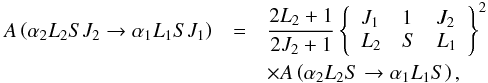 (30)which is analogous for the collisional transition coefficients.
3.5.2. Elastic or quasi-elastic collisions
We denote in this way those collisions responsible for transitions between the Zeeman sublevels of a given level. In solar physics, as these transitions are not of the permitted radiative type, the major contribution is that of collisions with neutral hydrogen atoms. The level may also be split into fine or hyperfine sublevels. The transitions induced between these sublevels are also possible and taken into account. To do this, we recommend the formalism by Kerkeni (2002, Eqs. (16)–(18)), who generalizes that of Omont (1977). In these papers, the collisional transition rates are expressed in irreducible tensorial components. They have to be transformed into the dyadic components used in the present paper, for instance, by applying the basis transformation coefficients given by Landi Degl’Innocenti & Landolfi (2004, p. 123)
3.6. Transition from the Zeeman effect to the Paschen-Back effect
To take the transition from the Zeeman effect to the Paschen-Back effect (or incomplete Paschen-Back effect) into account, see Sect. 3 of Bommier (1980), and in particular to its Eq. (34), which has to be applied to the statistical equilibrium Eq. (9) in this case, and similarly for the transfer equation coefficients.
4. Comprehensive discussion
4.1. Is the statistical equilibrium system of equations to be resolved for each atomic velocity class?
It has been shown in Sect. 3.1 that the atomic density matrix also depends on external freedom degrees like the atomic velocity. The first step in answering the question above is to compare the duration between two changes of atomic velocity and the level lifetimes. First, different causes of changing atomic velocity may be considered: collisions with photons, collisions with electrons and collisions with other atoms or ions (heavy particles). We refer here to the excellent discussion about these effects in Landi Degl’Innocenti & Landolfi (2004, Sect. 13.2, p. 691).
4.1.1. The different collision classes
First, the atomic velocity may change by the recoil effect when a photon is emitted or absorbed. Landi Degl’Innocenti & Landolfi (2004) evaluate the atomic recoil in a photon absorption or emission to be on the order of 1.4 cm s-1, for an iron atom of atomic mass 56 and in the visible range λ = 5000 Å, which should be compared to velocities on the order of some km s-1 that are typically found in stellar atmospheres. The atomic recoil due to atom-photon interaction can then be ignored as a cause of atomic velocity change.
Second, the effect of collisions between the atom under interest and electrons has to be considered. In stellar atmosphere, these collisions are found to be responsible for inelastic transitions, by a majority. By “inelastic”, we mean that the initial and final levels of the transition are also those of a permitted spectral line. In this case, the electron-atom interaction potential behaves in 1 /r2, where r is the atom-electron distance, whereas in the case of a neutral atom-neutral atom collision, the interaction potential would behave in 1 /r6. This difference in the interaction potentials results in the dominant effect of the electron-atom collisions, for those inelastic collisions populating the upper level, which may then de-excite by emitting a photon. Thus, those inelastic collisions are the source of some radiation in the atmosphere. They are responsible for the ϵ = CJ′J/AJ′J coefficient of the radiative transfer equation, where C (resp. A) is the collisional (resp. radiative) de-excitation probability from the upper J′ level toward the lower J level. In stellar chromospheres one has typically ϵ ≈ 10-3−10-4 and higher values in the deeper layers. With respect to the target atom, electrons are light particles. Landi Degl’Innocenti & Landolfi (2004) show that the recoil of the atom due to an electron-atom collision is on the order of Δv/v ≈ 3.1 × 10⁻³ for an iron atom of atomic mass 56. This recoil can then also be neglected.
Third, the collisions between two neutral atoms have to be examined as for the so-called elastic collisions, which connect for instance Zeeman sublevels of the same atomic level. When a magnetic field is present, the Zeeman sublevels split in energy and the collisional transitions between them become “weakly inelastic”. Transitions between fine or hyperfine structure levels also fall in the category of the weakly inelastic collisions, which in the following we simply denote as “elastic collisions”. All these transitions correspond to forbidden spectral lines. In the case of such transitions that are collisional, their probability is on the order of 10-8−10-9NH s-1, for those collisions with neutral hydrogen atoms of density NHexpressed in cm-3, whereas the probability is on the order of 10-6−10-7Ne s-1 for those collisions with electrons of density Ne, which is also expressed in cm-3. In the solar photosphere where typically NH ≈ 1017 cm-3 and Ne ≈ 1014 cm-3, the result is the dominant effect of the neutral hydrogen-neutral atom collisions in the category of those elastic collisions. In the radiative transfer, those collisions are responsible for the balance between coherent and incoherent scatterings, globally denoted as PRD (partial redistribution), as shown by Omont et al. (1972). We return to this point in more detail in Sect. 4.2.
One has then to examine if those elastic collisions could be also responsible for an atomic velocity change. The atom could eventually change velocity direction only, without the velocity modulus changing, but this would also be a velocity change. The quantitative evaluation would result from the examination of the differential cross sections. As such cross sections are rare, in the thermal energy range typical of stellar atmospheres, an approached evaluation was proposed by Landi Degl’Innocenti & Landolfi (2004) by considering that the cross section is rarely larger than  , where a0 is the Bohr radius, which is reasonable. This leads to a minimum value of NH> 1020 cm-3, for a time between two such collisions equal to the level lifetime, for a level inverse lifetime A = 107 s-1, which is typical for excited levels. It is thus seen that such velocity-changing collisions form a subclass of the class of elastic collisions. For hydrogen colliders, the interaction potential is longer ranged than for other neutral atoms that are heavier and, in contrast, the collisions that are responsible for the atomic velocity change correspond to short-range interactions. This is why the velocity-changing collisions are a subclass of the elastic collision class. For collisions with atoms that are heavier than hydrogen, their densities are so much lower than that of hydrogen, that the effect is weaker. Given the above order of magnitude, it can be seen that the velocity-changing collisions may be ignored in the solar atmosphere for excited levels, even if this is not the case for the elastic collisions that are responsible for the PRD.
4.1.2. The statistical equilibrium equations and velocity-changing collisions
Consequently, as mentioned in Sect. 3.1, the density matrix ensemble of elements σ(v,t) is completely decoupled from the density matrix ensemble of elements σ(v′,t) when v′ ≠ v, at least for excited state elements. If such a coupling was not negligible, a collisional term would appear in the statistical equilibrium equation of a population or coherence ⟨αJM|σ(v,t)|α′J′M′⟩, coupling it to elements of σ(v′,t) with transition probabilities associated with these velocity-changing collisions. Oxenius (1986, see Sect 2.2.1) denotes such a coupling term as a generalized Boltzmann term.
This coupling term is also described by Landi Degl’Innocenti & Landolfi (2004) and Cooper et al. (1982), where expressions for this term are found. Many collisions would occur in the level before de-excitation if it were large, i.e., when the time between two velocity-changing collisions was short with respect to the level lifetime. As a consequence, the level would be thermalized and the level velocity distribution would be Maxwellian. The level velocity distribution is ⟨αJM|σ(v,t)|αJM⟩. We have shown, on the contrary, that these collisions are very rare in the excited levels in the solar atmosphere. As a consequence, the level velocity distribution may not be Maxwellian, at least in the excited levels. In the ground level, these collisions can be non-negligible because the lifetime of this level is much longer. They thermalize the level and the velocity distribution in this level remains close to the Maxwellian. As an example, we performed a numerical solution of the velocity-dependent statistical equilibrium, which we present in the following paper of this series (Bommier 2016). We chose the pair of Na i D lines for our example. At the temperature minimum height, we obtain a departure of 5% from the Maxwellian, in the excited levels. Higher in the atmosphere, i.e. in the chromosphere, the departure reaches 20%. We measure this departure as the standard deviation, normalized to the average value, of the ratio between the upper and lower level populations, as a function of the atomic velocity.
However, usually the statistical equilibrium equations (SEE) do not take any velocity dependence into account. This is the case for the equations presented by Milahas (1978), but he acknowledges that complete redistribution is assumed both in the second chapter after Eqs. (2)–(15) and when he introduces the statistical equilibrium equations at the beginning of Sect. 5-4. This is velocity redistribution and this means that the velocity distribution is Maxwellian, regardless of the atomic internal state. In other words, this means that each excited level velocity distribution is Maxwellian. Thus, this assumes that the velocity-changing collision rate is high with respect to the de-excitation rates. As the velocity-changing collisions are a subclass of the elastic collisions, the elastic collision rate is yet higher, and as such higher than any other rate. Thus, the redistribution is complete, in the usual meaning of this term, i.e., including the frequency redistribution in the atomic reference frame. If the elastic collision rates are high, they also depolarize the atomic levels, i.e., they destroy the atomic alignment that is responsible for the linear polarization of emitted lines. No polarization would survive to such rates so that studying the polarization in such a scheme would be would not make sense.
On the other hand, PRD is generally studied for two-level atoms by applying redistribution functions (Hummer 1962), which are transformed from the atomic reference frame to the laboratory reference frame by assuming a given and unchanged atomic velocity v. Because the velocity remains unchanged during the scattering process, which corresponds to diagram (1), (2), or (3) of Fig. 1 in delineating scattering amplitudes, and because the upper level intervenes with its finite lifetime even for diagram (3), it is assumed that the atomic velocity does not change along this lifetime. In other words, considering the usual redistribution functions expressed in the laboratory frame as done in Milahas (1978), is simply solving the two-level atom statistical equilibrium for the given velocity class. In the case of a two-level atom, there is only one equation in the system of statistical equilibrium equations, so that the solution is immediate. It is performed for the velocity class under consideration in a way that the usual redistribution functions correspond to the SEE resolution for each velocity class, which is associated with a very low, velocity-changing collision rate. If one studies PRD, the elastic collision rate is not expected to be high in order for frequency coherence to survive. Accordingly, the velocity-changing collision rate is consistently very low because the velocity-changing collisions are a subclass of the elastic collisions. Belluzzi et al. (2013) verified the agreement between redistribution functions of Hummer (1962), and the redistribution function resulting from the resolution of the velocity-dependent SEE.
In studies of multilevel atoms, some authors, for example, Uitenbroek (1989, 2001), give part of their model using the high velocity-changing collision rates hypothesis for resolving the usual SEE, as described in Milahas (1978), and part of their model using the opposite hypothesis of very low velocity-changing collision rates for applying the usual redistribution functions even if these redistribution functions are a generalization to three-level atom, such as those functions developed by Hubený et al. (1983a). This usage of opposite hypotheses may question self-consistency, but the effect is probably detectable in very limited cases. As the atom ground level is, by far, the most populated in the weak radiation field limit, the velocity distribution in this level remains Maxwellian, as assumed in the usual SEE. Thus, when PRD is considered for resonance or other lines starting from the ground level, the model remains consistent. Differences may arise only for subordinate lines, when the velocity distribution in the line lower level departs from the Maxwellian velocity distribution, which can occur only in excited levels. We obtained departures from the Maxwellian velocity distribution function up to 20% in the above reported case of the upper levels of the Na i D lines. Indeed, studying PRD is consistent with the very low velocity-changing collision rates, consequently the statistical equilibrium equations should rather be resolved for each atomic velocity class for consistency, but the numerical application of this has so far not been successful.
Another case can be found where the velocity-dependent SEE reduce to the usual SEE: this is the case of the flat incident radiation spectrum. When the incident radiation does not vary with frequency, each absorption or induced emission transition probability in the SEE may be frequency integrated because the only remaining dependence is that of the absorption or induced emission profile, whose integral is unity. As the velocity dependence is also included in this profile, the velocity dependence disappears after the profile frequency integration. Accordingly, the SEE coefficients all become velocity independent and, consequently, the level population velocity distribution functions are all identical and then Maxwellian. The flat spectrum approximation is introduced by Landi Degl’Innocenti & Landolfi (2004, p. 257), for complete redistribution purposes, but is related to frequency redistribution (see the next subsection) and line profiles. If the incident radiation spectrum contains spectral lines, the approximation of the flat spectrum would consist in assuming a very large incident line width with respect to the absorption profile Doppler width. This is not the case, in practice, where the incident line width is on the order of a few Doppler widths. Thus, velocity-independent SEE and flat spectrum approximation do not correspond to practical stellar applications.
Interesting and related comments about the velocity redistribution can be found in Hubený et al. (1983b). They consider that “no elastic velocity-changing collisions occur during the time when the atom is excited (correlated re-emission)”, and that “the velocity of the atom is not affected by the interaction with perturber particles that leads to collision broadening of the atomic level”. As a consequence, “the ensemble of atoms that have velocities in an infinitesimal range d3v around the velocity v forms a group of atoms which can be considered independently of all the other atoms that have velocities outside this range”. They also mention the natural population phenomenon. As far as we understand this concept, a level is naturally populated, if the populating process is independent of the atomic velocity, such as the spontaneous emission or the absorption of a flat spectrum. Thus, natural populating processes do not modify the level population velocity distribution or copy this distribution from the lower (resp. upper) level to the upper (resp. lower) level. They comment as follows: “absorptions and stimulated emissions in spectral lines lead to deviations from natural population if the radiation intensity varies within the spectral line”.
4.2. Two different physical mechanisms, governed by nearly the same collisional condition, are responsible for PRD
Two different and independent physical mechanisms are responsible for the so-called redistribution. Sometimes, one considers redistribution in frequency in the atomic reference frame, on the one hand, and redistribution in velocity or Doppler redistribution in the laboratory reference frame, on the other hand. These two types of redistribution correspond to two distinct physical mechanisms. The first is based on the Rayleigh/Raman scattering, or coherent scattering, which is more important in the line far wings, and is ignored when one considers line absorption and emission forming the resonant scattering and described by transition probabilities. As for the transition amplitudes, the Rayleigh/Raman scattering is represented by diagram (3) of Fig. 1. The Rayleigh/Raman scattering is frequency coherent, i.e., the frequency of the scattered photon is in close relation with the frequency of the incident photon, taking an eventual change of internal atomic state for the Raman scattering into account. On the contrary, there is a priori no frequency coherence in the resonant scattering. The balance between these two scatterings has been studied by the pioneer work of Omont et al. (1972), who provide similar diagrams that are also based on a quantum mechanical approach.
Independently, the Doppler effect may be responsible for a relation between the frequency of the photon impinging an atom of velocity v, and that of the photon emitted in another direction by the same atom of velocity v. Accounting for the correlated Doppler effect is responsible for the Doppler redistribution. It is at the basis of the redistribution function calculation in the laboratory frame as reported by Milahas (1978) and of the scattering studied by Hubený et al. (1983b).
These two effects, Rayleigh/Raman scattering on the one hand and Doppler coherence on the other hand, are different and independent, but are both responsible for the redistribution in scattering. Their importance is governed by the same collisions: the so-called elastic collisions, which induce transitions between the Zeeman sublevels or fine or hyperfine structure levels, and are in the majority owing to collisions of the atom with neutral hydrogen in stellar atmospheres. Because of this similarity and similarities in the consequences, for instance, the fact that for complete redistribution the redistribution function is given or can be approximated by the product of incident and emitted frequency profiles, and also because both effects contribute to the redistribution function, the effect of interest is not always immediately clear when redistribution is in question. We found that the work by Cooper et al. (1982) takes both effects into account in a clear manner. In addition these authors introduce the eventual generalized Boltzmann term that couples atoms of different velocities.
These two effects are different and independent, but they are coupled in the redistribution by the fact that their importance is governed by the importance of the same collisions, which thus creates a link between them in redistribution.
4.3. The specificities of our formalism of the multilevel scattering
Our formalism presented in this paper takes both frequency and velocity redistributions into account. As our formalism is based on the Schrö dinger equation for the atom-radiation interaction, it does not make use of any redistribution function nor of different and specific absorption and emission profiles, as is usually done when studying PRD. They are in some ways replaced by the second term of the emissivity ε(4)(ν,Ω) as defined in Eq. (1), which is the contribution of taking the Rayleigh/Raman scattering into account. As for the Doppler coherence, it is taken into account by solving the statistical equilibrium equations for each atomic velocity class. The integration over atomic velocities is performed in each coefficient of the radiative transfer equation, which is then derived in the laboratory frame.
4.4. Comment on the common treatment of multilevel atom and scattering
Scattering and the multilevel atom are not easy to manage together. Ignoring for a moment the Zeeman sublevel structure and polarization, scattering does not modify the atomic state because a photon is absorbed and then or at the same time is re-emitted, so that the atomic state does not change when scattering is considered as a process as a whole. Studying scattering does then not easily incorporate the statistical equilibrium of the atomic levels, which assumes transitions between the levels. This is the reason why Casini et al. (2014) do not obtain any statistical equilibrium equation.
We consider a two-level atom and ignore Zeeman structure and polarization for a moment. Scattering does not change the atomic state. The lower level population is then unchanged by scattering, and, therefore, is determined by the initial conditions. In terms of the number of interaction Hamiltonians entering the process probability, it is an order-4 process as those studied by Casini et al. (2014). If one studies only order-2 processes on the contrary, those are separate and independent absorption and emission of a photon. In this case, there are transitions between the upper and lower levels. As a consequence, a statistical equilibrium equation may be written based on those transitions. It then appears that, similarly, the order-6 development of the Schrödinger equation would again lead to a possible statistical equilibrium equation because the order-6 process between two levels would result in a global transition between them as the initial and final states would be again different, but order-8 would not, and so on. Odd orders would then produce a statistical equilibrium equation, whereas even orders would not because in this case the atomic state would not change under the process. This behavior, which could induce some doubts about the possibility of convergence, has to be considered in the following general frame that the atom state is not measured by the observations. The retrieved information results from the photon analysis, but the atom state remains out of reach of the observation or experiment. In this paper, we have presented a solution to this problem by transforming the suite of orders into a perturbation série to be added up by taking each process in its “native” order. This has led to our model, which is no more than a model that gives us an account of the observed polarized radiation. It would be very difficult to build an alternative model for a multivel atom without any statistical equilibrium equation because complicate multilevel processes would have to be identified for which it is very difficult to write down a general expression.
5. Conclusions
In this paper, we have presented a generalized formalism that is able to account for both Rayleigh/Raman and resonant scatterings by a multilevel and multiline model atom. Thus, far wings and line cores are obtained for the spectral lines. The important new result is that the statistical equilibrium equations for the atomic density matrix elements have to be resolved for each atomic velocity class. In other words, there is one statistical equilibrium system of equations to resolve per atomic velocity. The radiative transfer equation coefficients are also provided, which include the integration of the atomic density matrix elements over the atomic velocity distribution function.
An example of the coupled resolution of both equations for non-LTE modeling is provided in the following paper of this series (Bommier 2016) for the case of the Na i D1 and D2 lines observed close to the solar limb in the second solar spectrum.
Acknowledgments
The author is grateful to the referee, H. Uitenbroek, for his review, and to N. Feautrier and S. Sahal-Bréchot for fruitful discussions.
References
- Baranger, M. 1958, Phys. Rev., 111, 494 [NASA ADS] [CrossRef] [MathSciNet] [Google Scholar]
- Belluzzi, L., & Landi Degl’Innocenti, E. 2009, A&A, 495, 577 [NASA ADS] [CrossRef] [EDP Sciences] [Google Scholar]
- Belluzzi, L., & Trujillo Bueno, J. 2014, A&A, 564, A16 [NASA ADS] [CrossRef] [EDP Sciences] [Google Scholar]
- Belluzzi, L., Landi Degl’Innocenti, E., & Trujillo Bueno, J. 2013, A&A, 552, A72 [NASA ADS] [CrossRef] [EDP Sciences] [Google Scholar]
- Bommier, V. 1997a, A&A, 328, 706 [NASA ADS] [Google Scholar]
- Bommier, V. 1997b, A&A, 328, 726 [NASA ADS] [Google Scholar]
- Bommier, V. 1980, A&A, 87, 109 [NASA ADS] [Google Scholar]
- Bommier, V. 2016, A&A, 591, A60 [NASA ADS] [CrossRef] [EDP Sciences] [Google Scholar]
- Bommier, V., & Sahal-Brechot, S. 1978, A&A, 69, 57 [NASA ADS] [Google Scholar]
- Bommier, V., & Sahal-Bréchot, S. 1991, Ann. Phys., 16, 555 [Google Scholar]
- Casini, R., Landi Degl’Innocenti, M., Manso Sainz, R., Landi Degl’Innocenti, E., & Landolfi, M. 2014, ApJ, 791, 94 [NASA ADS] [CrossRef] [Google Scholar]
- Cohen-Tannoudji, C. 1977, in Frontiers in Laser Spectroscopy, Les Houches, Session XXVII, 1975, eds. R. Balian, S. Haroche, & S. Liberman (North-Holland, Amsterdam), 3 [Google Scholar]
- Cohen-Tannoudji, C., & Reynaud, S. 1977, J. Phys. B At. Mol. Phys., 10, 345 [NASA ADS] [CrossRef] [Google Scholar]
- Cooper, J., Ballagh, R. J., Burnett, K., & Hummer, D. G. 1982, ApJ, 260, 299 [NASA ADS] [CrossRef] [Google Scholar]
- Faurobert, M. 1987, A&A, 178, 269 [NASA ADS] [Google Scholar]
- Faurobert, M. 1988, A&A, 194, 268 [NASA ADS] [Google Scholar]
- Faurobert, M., Derouich, M., Bommier, V., & Arnaud, J. 2009, A&A, 493, 201 [NASA ADS] [CrossRef] [EDP Sciences] [Google Scholar]
- Gandorfer, A. 2000, The Second Solar Spectrum: A high spectral resolution polarimetric survey of scattering polarization at the solar limb in graphical representation, Vol. I: 4625 Å to 6995 Å [Google Scholar]
- Gandorfer, A. 2002, The Second Solar Spectrum: A high spectral resolution polarimetric survey of scattering polarization at the solar limb in graphical representation, Vol. II: 3910 Å to 4630 Å [Google Scholar]
- Gandorfer, A. 2005, The Second Solar Spectrum: A high spectral resolution polarimetric survey of scattering polarization at the solar limb in graphical representation, Vol. III: 3160 Å to 3915 Å [Google Scholar]
- Grynberg, G., & Cagnac, B. 1977, Rep. Prog. Phys., 40, 791 [NASA ADS] [CrossRef] [Google Scholar]
- Hubený, I., Oxenius, J., & Simonneau, E. 1983a, J. Quant. Spec. Radiat. Transf., 29, 495 [NASA ADS] [CrossRef] [Google Scholar]
- Hubený, I., Oxenius, J., & Simonneau, E. 1983b, J. Quant. Spec. Radiat. Transf., 29, 477 [Google Scholar]
- Hummer, D. G. 1962, MNRAS, 125, 21 [NASA ADS] [CrossRef] [Google Scholar]
- Kerkeni, B. 2002, A&A, 390, 783 [Google Scholar]
- Kerkeni, B., & Bommier, V. 2002, A&A, 394, 707 [NASA ADS] [CrossRef] [EDP Sciences] [Google Scholar]
- Landi Degl’Innocenti, E., & Landolfi, M. 2004, Polarization in Spectral Lines (Kluwer Academic Publishers), Astrophys. Space Sci. Libr., 307 [Google Scholar]
- Loudon, R. 1973, The quantum theory of light (Oxford: Clarendon Press) [Google Scholar]
- Louisell, W. 1973, Quantum Statistical Properties of Radiation (New York: Wiley) [Google Scholar]
- Manso Sainz, R., & Trujillo Bueno, J. 2003, Phys. Rev. Lett., 91, 111102 [NASA ADS] [CrossRef] [Google Scholar]
- Milahas, D. 1978, Stellar Atmospheres, 2nd edn. (San Francisco: Freeman & Co) [Google Scholar]
- Omont, A. 1977, Prog. Quant. Electron., 5, 69 [Google Scholar]
- Omont, A., Smith, E. W., & Cooper, J. 1972, ApJ, 175, 185 [Google Scholar]
- Oxenius, J. 1986, Springer Series in Electrophysics, Vol. 20, Kinetic theory of Particles and Photons, Theoretical Foundations of Non-LTE Plasma Spectroscopy (Berlin: Springer-Verlag) [Google Scholar]
- Sahal-Bréchot, S., & Bommier, V. 2014, Adv. Space Res., 54, 1164 [NASA ADS] [CrossRef] [Google Scholar]
- Sahal-Brechot, S., Bommier, V., & Feautrier, N. 1998, A&A, 340, 579 [NASA ADS] [Google Scholar]
- Sampoorna, M., Nagendra, K. N., & Stenflo, J. O. 2013, ApJ, 770, 92 [NASA ADS] [CrossRef] [Google Scholar]
- Seaton, M. J. 1962, in Atomic and Molecular Processes, ed. D. R. Bates (New York: Academic Press) [Google Scholar]
- Smitha, H. N., Sampoorna, M., Nagendra, K. N., & Stenflo, J. O. 2011, ApJ, 733, 4 [NASA ADS] [CrossRef] [Google Scholar]
- Smitha, H. N., Sowmya, K., Nagendra, K. N., Sampoorna, M., & Stenflo, J. O. 2012, ApJ, 758, 112 [NASA ADS] [CrossRef] [Google Scholar]
- Smitha, H. N., Nagendra, K. N., Sampoorna, M., & Stenflo, J. O. 2013, J. Quant. Spec. Radiat. Transf., 115, 46 [NASA ADS] [CrossRef] [Google Scholar]
- Stenflo, J. O., & Keller, C. U. 1997, A&A, 321, 927 [NASA ADS] [Google Scholar]
- Uitenbroek, H. 1989, A&A, 213, 360 [NASA ADS] [Google Scholar]
- Uitenbroek, H. 2001, ApJ, 557, 389 [NASA ADS] [CrossRef] [Google Scholar]
All Figures
|
Fig. 1 Elementary processes and transition probabilities for the master equation developed at order-2 (upper part) and order-4 (lower part). At order-4, diagrams (1) and (2) are combinations of the order-2 elementary processes, whereas diagram (3) and (4) are not. |
| In the text | |
Current usage metrics show cumulative count of Article Views (full-text article views including HTML views, PDF and ePub downloads, according to the available data) and Abstracts Views on Vision4Press platform.
Data correspond to usage on the plateform after 2015. The current usage metrics is available 48-96 hours after online publication and is updated daily on week days.
Initial download of the metrics may take a while.