| Issue |
A&A
Volume 590, June 2016
|
|
|---|---|---|
| Article Number | A84 | |
| Number of page(s) | 6 | |
| Section | Planets and planetary systems | |
| DOI | https://doi.org/10.1051/0004-6361/201628334 | |
| Published online | 16 May 2016 | |
Chromatic line-profile tomography to reveal exoplanetary atmospheres: application to HD 189733b
INAF–Osservatorio Astronomico di Brera,
via E. Bianchi 46, 23807
Merate ( LC), Italy
e-mail:
francesco.borsa@brera.inaf.it
Received: 18 February 2016
Accepted: 25 March 2016
Context. Transmission spectroscopy can be used to constrain the properties of exoplanetary atmospheres. During a transit, the light blocked from the atmosphere of the planet leaves an imprint in the light coming from the star. This has been shown for many exoplanets with both photometry and spectroscopy, using different analysis methods.
Aims. We test chromatic line-profile tomography as a new tool to investigate exoplanetary atmospheres. The signal imprinted on the cross-correlation function (CCF) by a planet transiting its star is dependent on the planet-to-star radius ratio. We want to verify whether the precision reachable on the CCF obtained from a subset of the spectral orders of the HARPS spectrograph is high enough to determine the radius of a planet at different wavelengths.
Methods. We analyze HARPS archival data of three transits of HD 189733b. We divide the HARPS spectral range into seven broadbands, calculating for each band the ratio between the area of the out-of-transit CCF and the area of the signal imprinted by the planet on it during the full part of the transit. We take into account the effect of the limb darkening using the theoretical coefficients of a linear law. Averaging the results of three different transits allows us to obtain a good-quality broadband transmission spectrum of HD 189733b with a greater precision than that of the chromatic Rossiter McLaughlin effect.
Results. We proved that chromatic line-profile tomography is an interesting way to reveal broadband transmission spectra of exoplanets: our analysis of the atmosphere of HD 189733b is in agreement with other ground- and space-based observations. The independent analysis of different transits emphasizes the probability that stellar activity plays a role in the extracted transmission spectrum. Therefore, care should be taken when claiming that Rayleigh scattering is present in the atmosphere of exoplanets orbiting active stars using only one transit.
Key words: techniques: spectroscopic / planets and satellites: atmospheres / planetary systems
© ESO, 2016
1. Introduction
The number of discovered exoplanets has grown exponentially in recent years thanks to many ground- and space-based surveys that take advantage of different methods of detection (e.g., Wright & Gaudi 2013). The existence of exoplanets and their abundance in our galaxy has been firmly established, and now the attention of the scientific community is moving to exoplanet characterization and atmospheric content. During a planetary transit, a fraction of the light coming from the host star is filtered through the planet’s atmosphere, thus providing hints of its composition. The atmospheric depth at which the stellar light becomes extinct depends on the wavelength and atmospheric composition, and if an atom or molecule is present, the planet becomes opaque in the respective absorption band resulting in a larger obscured area. As a consequence, the eclipse appears deeper at the wavelength of the absorption band, yielding what appears to be a larger radius. The study of this effect, i.e., transmission spectroscopy, has been demonstrated to be a very successful technique for investigating exoplanetary atmospheres (Burrows 2014).
HD 189733b (Bouchy et al. 2005) represents the perfect science case for testing new methods aimed at identifying its transmission spectrum. The brightness of its host star (MV = 7.67) and the depth of its transit (>2%) allows us to reach a high signal-to-noise ratio (S/N). Its atmosphere at optical wavelengths has been explored with many different methods using primary transit, with both ground- and space-based observations. From Earth, Redfield et al. (2008) were the first to detect sodium absorption using the High Resolution Spectrograph on the Hobby-Eberly telescope. Later, Wyttenbach et al. (2015) were able to show the signal of atomic sodium and Louden & Wheatley (2015) retrieved the velocity of winds on both hemispheres of the planet with HARPS. With the same observations Di Gloria et al. (2015) probed the Rayleigh scattering slope by using the chromatic Rossiter-McLaughlin (RM) effect. McCullough et al. (2014) claimed that stellar activity is the main cause of the slope observed in the transmission spectrum. From space, Pont et al. (2008) with ACS and Sing et al. (2011) with STIS detected Rayleigh scattering using the Hubble Space Telescope (HST). Pont et al. (2013) presented a homogeneous reanalysis of the data and a global transmission spectrum from ultraviolet to infrared. Huitson et al. (2012) were able to detect and characterize sodium in the atmosphere.
Each surface element of a rotating star has a specific radial velocity. If there is a reduction of flux from a region, for example for the presence of a spot or for the obscuration by a transiting planet, the contribution to the stellar line-profile at this velocity will be affected, resulting in the presence of a bump in the line profile. As the transiting planet moves across the disk, this perturbation will move across the line profile because the radial velocity of the obscured zone is different. The analysis of this effect, called line-profile tomography, has been very useful for detecting the inclination of the orbital plane of the planet with respect to the stellar rotational axis (e.g., Collier Cameron et al. 2010a,b), for the confirmation of the presence of exoplanets (Hartman et al. 2015), and for the measurement of their nodal precession (Johnson et al. 2015). This has been done in particular for high Veqsini stars because for these stars it is more difficult to extract precise radial velocities and analyze the RM effect. Line-profile variation studies have also been widely used in the study of the stars themselves, with asteroseismology. The spectral lines of a pulsating variable show variable mean line profiles. By measuring the observed variations, it is possible to typify the excited modes by assigning the spherical wavenumbers (l,m) to each of them (e.g., Poretti et al. 2013).
To compare the atmospheric properties between different exoplanets and subsequently identifying possible subclasses, we need to observe as many exoplanetary atmospheres as possible. Given the difficulty of this kind of observations, any new method of investigation that can increase the sample is welcome. In this paper, we describe the chromatic line-profile tomography as a new method for obtaining broadband transmission spectroscopy of exoplanetary atmospheres. We test it by using the well-known case of the transiting exoplanet HD 189733b and by comparing the results with its transmission spectra obtained from other analyses.
2. HARPS data and choice of broadbands
As in previous atmospheric analyses of ground-based data of HD 189733b, we used the three full transits observed spectroscopically with HARPS available in the ESO archive and obtained under programs 072.C-0488(E), 079.C-0127(A), and 079.C-0828(A). An observations log, together with the number of exposures and exposure times for each transit, is available in Wyttenbach et al. (2015, see their Table 1).
HARPS (Mayor et al. 2003) is a fiber-fed echelle spectrograph composed of 72 orders in a range of wavelength from 378 nm to 691 nm and a resolving power R ≃ 115 000. The HARPS Data Reduction Software (DRS) estimates the radial velocities (RVs) of the targets by computing cross-correlation functions (CCFs, Baranne et al. 1996; Pepe et al. 2002) between a weighted line mask and the stellar spectrum for each order and then summing them together. To avoid contamination from the telluric lines, the masks do not have any reference lines in the wavelength ranges where the terrestrial atmospheric contribute is very large, which means that there is no CCF at all for three orders of the spectra (orders 89, 94, and 103).
The method we are testing here uses CCFs obtained from different subsets of orders. We chose to use the same division of orders as has been used by Di Gloria et al. (2015) in order to better check our results and the reliability of our method (see Table 1). After a first analysis, we considered that the use of the first nine orders (up to the Ca ii H&K spectral region) could led to unreliable results. The Ca ii H&K lines are, in fact, particularly variable in the case of active stars (such as HD 189733, Boisse et al. 2009), and are often used as tracers for the level of stellar activity (e.g., Borsa et al. 2015). The emission present in their core could thus influence the shape of the CCF. Moreover, the S/N of these orders is much lower than in the others for the star analyzed; this is due to the low efficiency of the instrument at these wavelengths and to the spectral type of the star (K1-K2, Bouchy et al. 2005). Stellar and transit parameters used during this analysis are listed in Table 2.
Wavelength ranges for the order groups considered, and the respective linear limb darkening coefficient used.
Stellar and transit parameters used in this work.
3. Chromatic line-profile tomography
The morphology of the CCF changes when a planet transits in front of the star: the Gaussian profile is no longer symmetric, and this asymmetry causes a systematic deviation when measuring the velocity centroid of the starlight. This effect – the Rossiter-McLaughlin effect – causes a spurious deviation of the RV measurements from the pure Keplerian motion, which is known to be an artifact of the asymmetry just described.
In the CCF, the missing light during the full part of the transit of a planet can be expressed with the formula (Eq. (9) in Collier Cameron et al. 2010a): 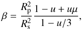 (1)where
  , with d the distance of the planet from the center of the star in stellar radius units, and u the coefficient of linear limb darkening. We note here that β depends on the planet-to-star radius ratio (Rp/Rs) (see Collier Cameron et al. 2010a, for details).
The limb darkening (LD) coefficients for the wavelength ranges of our chosen order groups, listed in Table 1, were calculated using the code LDTK (Parviainen & Aigrain 2015), which generates custom LD coefficients and the relative uncertainties with a library of PHOENIX-generated specific intensity spectra (Husser et al. 2013). We assumed here that both the mean line profile of the star and the shadow caused by the planet could be modeled with a Gaussian function.
3.1. Data analysis
We computed a separate analysis for each transit in order to be free from the systematics that arise from different nights of observations that can perturb the CCF shape (e.g., terrestrial atmospheric conditions). In addition, using this approach means that we can compare the transmission spectra obtained on different nights and investigate the possibility that stellar activity can influence the retrieval of the transmission spectrum. It has been suggested, in fact, that the Rayleigh scattering claimed in the planet’s atmosphere is just an artifact caused by stellar activity (McCullough et al. 2014).
As a first step, for each spectrum we computed the predicted RV of the host star relative to the pure Keplerian motion without the apparent deviation caused by the RM. To do this we computed a linear fit using the DRS-estimated RVs of the out-of-transit spectra, and used this line as our reference for the Keplerian motion of the star caused by the planet.
Then we applied our new procedure to each broadband chosen in Table 1. We extracted the CCFs relative to the orders of the broadband we analyzed from the CCF fits files generated by the HARPS DRS pipeline. These CCFs were then averaged and normalized, thus creating one CCF per spectrum for each broadband. The normalization was done in the same way for all the CCFs, with a linear fit between all the points with v< −15 km s-1 or v> 15 km s-1, thus including only the continuum in the fit. We also changed the limit value to 13 km s-1 and 17 km s-1 without significant differences in the final results. Hereafter, we refer to these CCFs relative to the group of orders. We created the reference CCF for the star (CCFref) by averaging all the CCFs of the out-of-transit spectra (Fig. 1), shifted for the relative RVs (as estimated from the pure Keplerian motion). No significant offset among different groups was detected (Fig. 1). We fitted the CCFref with a Gaussian function using the IDL function GAUSSFIT, and subsequently we calculated its area as  , where a and c are the height and the standard deviation of the Gaussian, respectively. The Spearman test did not detect any significant correlation between them. Hence, we also gave the errorbars for the area by propagating the errors on the a and c parameters obtained from the fits.
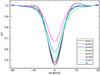 |
Fig. 1 Reference CCFs for the different groups of orders for the night Aug. 28, 2007. |
The CCFref was then subtracted from all the CCFs of every exposure. Special care was taken while normalizing the data inside the transit: the decrease in the photometric flux was taken into account (as in Cegla et al. 2016), using a transit model created with the formalism of Mandel & Agol (2002) and the transit parameters of Table 2. The data now show the typical Doppler shadow of the planet passing in front of the star (Fig. 2).
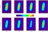 |
Fig. 2 Shadow of the planet over the stellar CCF for the night Aug. 28, 2007, in the different order groups (Table 1) and in the total HARPS passband. Top: left to right, shadow for the groups 1 to 4. Bottom: left to right, shadow for the groups 5 to 7, plus the total HARPS passband. The color scale, chosen for viewing ease, is the same in all the plots. |
From this point on we used only the data that are inside the full part of the transit. On each of the residual data we fitted a Gaussian profile, estimating its area in the same way as was done for Aref. We paid particular attention to check that the Gaussian profile was centered where the signal of the planet was expected. Because this signal was very low, in particular when using a small number of orders, this step was important in order to avoid that the Gaussian profile we were fitting was centered on a random noise bump instead of on the planetary one.
We then divided these areas for Aref, thus obtaining for each exposure inside the full part of the transit a value for the parameter β (see Eq. (1)). Because we knew a priori the position of the planet on the stellar disk and the limb darkening coefficients, we divided each β by the relative second term of Eq. (1). For each in-full-transit spectrum we then had an estimate of the ratio (Rp/Rs)2 (Fig. 3). We finally averaged these values taking as uncertainty their rms.
It is interesting to note that in a few cases the measurements show a clear linear trend as a function of the distance from the center of the star, probably because the given LD coefficient in use was not completely representative of the star at that moment at that wavelength. In fact, it has been demonstrated that the LD coefficients are also dependent on the particular situation of the star at the moment of observation (e.g., on the number and size of star spots, Csizmadia et al. 2013). In turn, this kind of analysis could be also useful to constrain the LD coefficients of the star.
We repeated the whole procedure for each broadband and for each transit. In this way we obtained one transmission spectrum per transit. Finally, we averaged the values of the same broadband, obtaining the final average transmission spectrum of HD 189733b (Table 3, Fig. 4).
Values of Rp/Rs for HD 189733b obtained in this work using the chromatic line-profile tomography technique.
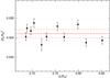 |
Fig. 3 Example of the values of (Rp/Rs)2 found for one broadband as a function of the distance of the planet from the center of the star (d). The red line represents the average (Rp/Rs)2 taken as the final value; the dashed lines define its uncertainties. |
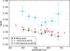 |
Fig. 4 Broadband transmission spectrum of HD 189733b as calculated with this method (black circles). For comparison, red triangles are HST observations by Pont et al. (2013) and light blue squares are measurements from Di Gloria et al. (2015) using the chromatic RM effect on the same dataset of this paper. The vertical shift is due to the different transit parameters used in the different papers. |
4. Discussion
Our Rp/Rs values derived with chromatic line-profile tomography are in good agreement with those reported by other analyses (Fig. 4). There is a decrease in Rp/Rs going toward longer wavelengths that closely matches the slope of the HST data of Pont et al. (2013). We did not take into account their correction for star spots since it is well inside our errorbars. Our uncertainties are of course larger than the ones obtained with HST, but one-half smaller than those obtained by Di Gloria et al. (2015) who analyzed the same dataset using a different analysis method. The uncertainties could be reduced by increasing the number of observed transits; this should be easier with ground-based observations than from space.
4.1. Comparison of single transit events
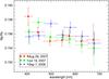 |
Fig. 5 Broadband transmission spectroscopy of HD 189733b calculated for the single transit events recorded with HARPS. Red circles refer to the transit of Aug. 28, 2007; green squares to Jul. 19, 2007; and blue triangles to Sep. 07, 2006. The wavelengths for the different transits are slightly shifted for graphic clarity. |
As mentioned before, the obtained transmission spectrum does not account for any kind of variation that arises from occulted and unocculted star spots. These can affect the CCF, modifying its shape in the same way as the transit of a planet does. As happens in a transit, star spots occulted by the planet during the transit can result in an underestimation of the planetary radius, while unocculted ones can lead to an overestimation; this effect is chromatic, and will thus be different depending on the wavelength. For this system, this effect has been largely analyzed by different authors who dispute that the slope seen in the transmission spectrum is due to Rayleigh scattering, to stellar activity, or both (Sing et al. 2011; Pont et al. 2013; Oshagh et al. 2014; McCullough et al. 2014). The detailed study of stellar activity is beyond the scope of the paper, but it is interesting to look at the results obtained in the independent analyses of the three different transits (Fig. 5). While the results at λ> 500 nm are in agreement, we note high variability in the blue part of the spectrum (λ< 500 nm). Given the high stability demonstrated by HARPS (e.g., Lovis et al. 2006), on the basis of our analysis we note that this variability could be due to different causes:
-
terrestrial atmosphere: variation in the observing conditions from night to night (e.g., variable seeing, weather) could induce subtle effects on the CCFs (e.g., Cosentino et al. 2014), thus influencing the results;
-
instrumental systematics: in the zone of lower S/N, due to both the spectral energy distribution of the star and the lower efficiency of the instrument, possible systematics could arise between different nights in the CCFs computation;
-
exoweather variability: the data are taken at different times, so in principle variations of planetary radius could be attributed to intrinsic variations in the atmosphere of the planet. This hypothesis is unlikely, however;
-
stellar activity: occulted and unocculted star spots affect this kind of measurements in a wavelength-dependent way. The number of spots on the stellar surface obviously changes with time, so their influence on the transmission spectrum can vary for each transit.
4.2. Sodium
The sodium D-lines (588.995 nm and 589.592 nm) have already been observed in the atmosphere of HD 189733b, in particular using the same dataset as used in this paper (e.g., Wyttenbach et al. 2015). By looking at Fig. 4, it is possible to see in our results a slight deviation from the decreasing radius toward longer wavelengths for the point relative to group 5, which matches in wavelength the variation given by the sodium doublet evident in the measurements from Pont et al. (2013). We note however that this deviation is not directly due to sodium: the sodium D-lines are in fact absent in the HARPS line masks and thus they do not contribute to the CCFs and to our analysis. In our opinion, it is also unlikely that the extended wings of planetary sodium absorption play a role in this slight increase.
5. Conclusions
We tested a new method for retrieving the broadband transmission spectrum of transiting exoplanets, proving that chromatic line-profile tomography during transit is a useful tool that provides insights on their atmospheres. We applied our method to existing high-quality high-resolution transit spectroscopic observations of HD 189733b, together with HD 209458b the most often studied exoplanet to date. The analysis of three transits observed with HARPS results in an averaged transmission spectrum that is in good agreement with the spectrum obtained from space (Pont et al. 2013), confirming that ground-based high-resolution spectrographs can be used to investigate the broadband transmission spectra of exoplanets.
Comparing the independent results from the three transits analyzed one by one, we can see a disagreement increasing toward the blue part of the spectrum. Even if we cannot completely exclude systematics, the most probable explanation is that stellar activity plays a role when extracting transmission spectra of exoplanets; therefore, care should be taken when using only one transit to claim Rayleigh scattering in the atmosphere of planets transiting active stars. Our technique matches the requirement to perform several observations at the same wavelength to quantify the effects of the stellar activity (Oshagh et al. 2014), with the advantage that it uses the entire optical spectrum to cross-check the results, which means that it is a valid alternative to multicolor photometry. With respect to the use of chromatic RM (Di Gloria et al. 2015), chromatic line-profile tomography has the advantage that it will be useful even in the case of planets transiting high Veqsini stars for which it is difficult to estimate precise RV values. The creation of a custom mask for the CCF estimation (e.g., Borsa et al. 2015) will help to further increase the precision of the results.
Future high-resolution spectrographs like ESPRESSO (Pepe et al. 2013) will provide a gain in the S/N, allowing us to use this method on fainter targets as well. Observation of as many planetary atmospheres as possible is needed for a comprehensive understanding of atmospheric properties, and any new technique can be useful for this scope.
Acknowledgments
We thank the referee for the careful reading of the manuscript and for the interesting checks suggested. Based on observations made with ESO Telescopes at the La Silla Paranal Observatory under programme IDs 072.C-0488(E), 079.C-0127(A) and 079.C-0828(A). F.B. acknowledges financial support from INAF through the “Progetti Premiali” funding scheme of the Italian Ministry of Education, University, and Research. M.R. acknowledges financial support from EU FP7 Collaborative Project SPACEINN: Exploitation of Space Data for Innovative Helio- and Asteroseismology.
References
- Baranne, A., Queloz, D., Mayor, M., et al. 1996, A&AS, 119, 373 [NASA ADS] [CrossRef] [EDP Sciences] [Google Scholar]
- Boisse, I., Moutou, C., Vidal-Madjar, A., et al. 2009, A&A, 495, 959 [NASA ADS] [CrossRef] [EDP Sciences] [Google Scholar]
- Borsa, F., Scandariato, G., Rainer, M., et al. 2015, A&A, 578, A64 [NASA ADS] [CrossRef] [EDP Sciences] [Google Scholar]
- Bouchy, F., Udry, S., Mayor, M., et al. 2005, A&A, 444, L15 [NASA ADS] [CrossRef] [EDP Sciences] [Google Scholar]
- Boyajian, T., von Braun, K., Feiden, G. A., et al. 2015, MNRAS, 447, 846 [NASA ADS] [CrossRef] [Google Scholar]
- Burrows, A. S. 2014, Nature, 513, 345 [NASA ADS] [CrossRef] [Google Scholar]
- Cegla, H. M., Lovis, C., Bourrier, V., et al. 2016, A&A, 588, A127 [NASA ADS] [CrossRef] [EDP Sciences] [Google Scholar]
- Collier Cameron, A., Bruce, V. A., Miller, G. R. M., et al. 2010a, MNRAS, 403, 151 [NASA ADS] [CrossRef] [Google Scholar]
- Collier Cameron, A., Guenther, E., Smalley, B., et al. 2010b, MNRAS, 407, 507 [NASA ADS] [CrossRef] [Google Scholar]
- Cosentino, R., Lovis, C., Pepe, F., et al. 2014, Proc. SPIE, 9147, 91478C [CrossRef] [Google Scholar]
- Csizmadia, S., Pasternacki, T., Dreyer, C., et al. 2013, A&A, 549, A9 [NASA ADS] [CrossRef] [EDP Sciences] [Google Scholar]
- Cutispoto, G., Pastori, L., Guerrero, A., et al. 2000, A&A, 364, 205 [NASA ADS] [Google Scholar]
- Di Gloria, E., Snellen, I. A. G., & Albrecht, S. 2015, A&A, 580, A84 [NASA ADS] [CrossRef] [EDP Sciences] [Google Scholar]
- Hartman, J. D., Bakos, G. Á., Buchhave, L. A., et al. 2015, AJ, 150, 197 [NASA ADS] [CrossRef] [Google Scholar]
- Huitson, C. M., Sing, D. K., Vidal-Madjar, A., et al. 2012, MNRAS, 422, 2477 [NASA ADS] [CrossRef] [Google Scholar]
- Husser, T.-O., Wende-von Berg, S., Dreizler, S., et al. 2013, A&A, 553, A6 [NASA ADS] [CrossRef] [EDP Sciences] [Google Scholar]
- Johnson, M. C., Cochran, W. D., Collier Cameron, A., & Bayliss, D. 2015, ApJ, 810, L23 [NASA ADS] [CrossRef] [Google Scholar]
- Louden, T., & Wheatley, P. J. 2015, ApJ, 814, L24 [NASA ADS] [CrossRef] [Google Scholar]
- Lovis, C., Pepe, F., Bouchy, F., et al. 2006, Proc. SPIE, 6269, 62690 [CrossRef] [Google Scholar]
- Mandel, K., & Agol, E. 2002, ApJ, 580, L171 [NASA ADS] [CrossRef] [Google Scholar]
- Mayor, M., Pepe, F., Queloz, D., et al. 2003, The Messenger, 114, 20 [NASA ADS] [Google Scholar]
- McCullough, P. R., Crouzet, N., Deming, D., & Madhusudhan, N. 2014, ApJ, 791, 55 [NASA ADS] [CrossRef] [Google Scholar]
- Oshagh, M., Santos, N. C., Ehrenreich, D., et al. 2014, A&A, 568, A99 [NASA ADS] [CrossRef] [EDP Sciences] [Google Scholar]
- Parviainen, H., & Aigrain, S. 2015, MNRAS, 453, 3821 [Google Scholar]
- Pepe, F., Mayor, M., Galland, F., et al. 2002, A&A, 388, 632 [NASA ADS] [CrossRef] [EDP Sciences] [Google Scholar]
- Pepe, F., Cristiani, S., Rebolo, R., et al. 2013, The Messenger, 153, 6 [NASA ADS] [Google Scholar]
- Pont, F., Knutson, H., Gilliland, R. L., Moutou, C., & Charbonneau, D. 2008, MNRAS, 385, 109 [NASA ADS] [CrossRef] [Google Scholar]
- Pont, F., Sing, D. K., Gibson, N. P., et al. 2013, MNRAS, 432, 2917 [NASA ADS] [CrossRef] [Google Scholar]
- Poretti, E., Rainer, M., Mantegazza, L., et al. 2013, in Stellar Pulsations: Impact of New Instrumentation and New Insights, Astrophys. Space Sci. Proc., 31, 39 [NASA ADS] [CrossRef] [Google Scholar]
- Redfield, S., Endl, M., Cochran, W. D., & Koesterke, L. 2008, ApJ, 673, L87 [NASA ADS] [CrossRef] [MathSciNet] [Google Scholar]
- Sing, D. K., Pont, F., Aigrain, S., et al. 2011, MNRAS, 416, 1443 [NASA ADS] [CrossRef] [Google Scholar]
- Strassmeier, K., Washuettl, A., Granzer, T., Scheck, M., Weber, M. 2000, A&AS, 142, 275 [NASA ADS] [CrossRef] [EDP Sciences] [Google Scholar]
- Torres, G., Winn, J. N., & Holman, M. J. 2008, ApJ, 677, 1324 [NASA ADS] [CrossRef] [Google Scholar]
- Triaud, A. H. M. J., Queloz, D., Bouchy, F., et al. 2009, A&A, 506, 377 [NASA ADS] [CrossRef] [EDP Sciences] [Google Scholar]
- Wright, J. T., & Gaudi, B. S. 2013, in Planets, Stars and Stellar Systems, Vol. 3: Solar and Stellar Planetary Systems (Springer), 489 [Google Scholar]
- Wyttenbach, A., Ehrenreich, D., Lovis, C., et al. 2015, A&A, 577, A62 [NASA ADS] [CrossRef] [EDP Sciences] [Google Scholar]
All Tables
Wavelength ranges for the order groups considered, and the respective linear limb darkening coefficient used.
Values of Rp/Rs for HD 189733b obtained in this work using the chromatic line-profile tomography technique.
All Figures
|
Fig. 1 Reference CCFs for the different groups of orders for the night Aug. 28, 2007. |
| In the text | |
|
Fig. 2 Shadow of the planet over the stellar CCF for the night Aug. 28, 2007, in the different order groups (Table 1) and in the total HARPS passband. Top: left to right, shadow for the groups 1 to 4. Bottom: left to right, shadow for the groups 5 to 7, plus the total HARPS passband. The color scale, chosen for viewing ease, is the same in all the plots. |
| In the text | |
|
Fig. 3 Example of the values of (Rp/Rs)2 found for one broadband as a function of the distance of the planet from the center of the star (d). The red line represents the average (Rp/Rs)2 taken as the final value; the dashed lines define its uncertainties. |
| In the text | |
|
Fig. 4 Broadband transmission spectrum of HD 189733b as calculated with this method (black circles). For comparison, red triangles are HST observations by Pont et al. (2013) and light blue squares are measurements from Di Gloria et al. (2015) using the chromatic RM effect on the same dataset of this paper. The vertical shift is due to the different transit parameters used in the different papers. |
| In the text | |
|
Fig. 5 Broadband transmission spectroscopy of HD 189733b calculated for the single transit events recorded with HARPS. Red circles refer to the transit of Aug. 28, 2007; green squares to Jul. 19, 2007; and blue triangles to Sep. 07, 2006. The wavelengths for the different transits are slightly shifted for graphic clarity. |
| In the text | |
Current usage metrics show cumulative count of Article Views (full-text article views including HTML views, PDF and ePub downloads, according to the available data) and Abstracts Views on Vision4Press platform.
Data correspond to usage on the plateform after 2015. The current usage metrics is available 48-96 hours after online publication and is updated daily on week days.
Initial download of the metrics may take a while.