| Issue |
A&A
Volume 590, June 2016
|
|
|---|---|---|
| Article Number | A64 | |
| Number of page(s) | 10 | |
| Section | Stellar structure and evolution | |
| DOI | https://doi.org/10.1051/0004-6361/201628181 | |
| Published online | 12 May 2016 | |
On the red giant branch mass loss in 47 Tucanae: Constraints from the horizontal branch morphology
1
Astrophysics Research Institute, Liverpool John Moores
University, IC2, Liverpool Science Park,
146 Brownlow
Hill,
Liverpool
L3 5RF,
UK
e-mail:
This email address is being protected from spambots. You need JavaScript enabled to view it.
2
INAF−Osservatorio
Astronomico di Teramo, via M. Maggini, 64100
Teramo,
Italy
e-mail: This email address is being protected from spambots. You need JavaScript enabled to view it.
, This email address is being protected from spambots. You need JavaScript enabled to view it.
3
Instituto de Astrofísica de Canarias, Calle via Lactea s/n, 38205, La Laguna, Tenerife, Spain
Received: 25 January 2016
Accepted: 10 April 2016
Abstract
We obtain stringent constraints on the actual efficiency of mass loss for red giant branch stars in the Galactic globular cluster 47 Tuc, by comparing synthetic modelling based on stellar evolution tracks with the observed distribution of stars along the horizontal branch in the colour-magnitude-diagram. We confirm that the observed, wedge-shaped distribution of the horizontal branch can only be reproduced by accounting for a range of initial He abundances, in agreement with inferences from the analysis of the main sequence, and a red giant branch mass loss with a small dispersion. We carefully investigated several possible sources of uncertainty that could affect the results of the horizontal branch modelling, stemming from uncertainties in both stellar model computations and cluster properties, such as heavy element abundances, reddening, and age. We determine a firm lower limit of ~0.17M⊙ for the mass lost by red giant branch stars, corresponding to horizontal branch stellar masses between ~0.65M⊙ and ~0.73M⊙ (the range driven by the range of initial helium abundances). We also derive that in this cluster the amount of mass lost along the asymptotic giant branch stars is comparable to the mass lost during the previous red giant branch phase. These results confirm, for this cluster, the disagreement between colour-magnitude-diagram analyses and inferences from recent studies of the dynamics of the cluster stars, which predict a much less efficient red giant branch mass loss. A comparison between the results from these two techniques applied to other clusters is required to gain more insights about the origin of this disagreement.
Key words: globular clusters: individual: 47 Tucanae / stars: evolution / stars: horizontal-branch / stars: low-mass / stars: mass-loss
© ESO, 2016
1. Introduction
Mass loss during the red giant branch (RGB) evolution of globular cluster (GC) stars has a generally negligible effect on their structure unless the RGB star is experiencing very high mass loss rates (Castellani & Castellani 1993). This mass loss is crucial, however, to interpreting the colour-magnitude-diagram (CMD) of the following horizontal branch (HB) phase, and affects the CMD and duration of the asymptotic giant branch (AGB) stage.
A comprehensive physical description of RGB mass loss processes is still lacking, and RGB mass loss rates are customarily parametrized in stellar evolution calculations by means of simple relations such as the Reimers formula (Reimers 1975) or, more recently, the Schröder & Cuntz (2005) formula. These prescriptions are essentially scaling relations between mass loss rates and global stellar parameters such as surface bolometric luminosity (L), gravity (g), effective temperature (Teff), and/or radius (R). The zero point of these scaling relations is typically set by a free parameter (η) that needs to be calibrated.
The more direct approach to study the mass loss in RGB stars is to detect outflow motions in the outer regions of the atmospheres, through the presence of asymmetries and coreshifts in chromospheric lines, (see e.g. Mauas et al. 2006; Vieytes et al. 2011), or detect the circumstellar envelopes at larger distances from the stars, for example through infrared dust emission (see e.g. Origlia et al. 2007, 2010; Boyer et al. 2010; Momany et al. 2012). Another traditional indicator of the efficiency of RGB mass loss is the CMD location and morphology of the HB of globular clusters, starting from the pioneering works by Iben & Rood (1970) and Rood (1973). Matching observed HBs with synthetic HB models traditionally requires that RGB stars lose a fraction of their initial mass with typical values of the order of ~0.2 M⊙ (see e.g. Lee et al. 1990; Catelan 1993; Salaris et al. 2007; di Criscienzo et al. 2010; Gratton et al. 2010; Dalessandro et al. 2013; McDonald & Zijlstra 2015, and references therein).
A very recent series of papers (Heyl et al. 2015b,a) has applied a completely different approach to estimate the mass lost by RGB stars in the Galactic GC 47 Tuc. Using HST images these authors determined the rate of diffusion of stars through the cluster core, using a sample of bright white dwarfs (WDs). They then compared the radial distribution of upper main sequence (MS), RGB, and HB stars, showing that they are nearly identical, even when only objects near the RGB tip are considered, whilst the radial distribution of young WDs is only slightly less concentrated than upper MS and RGB stars, indicating that there has been very little time for the young WDs to have diffused through the cluster since their progenitors lost mass. They estimated that most of the ~0.4 M⊙ that 47 Tuc stars lose between the end of the MS and the beginning of the WD sequence (the typical MS turn-off mass for 47 Tuc, as inferred from theoretical isochrones, is equal to ~0.9M⊙, whilst typical masses for bright WDs in GCs as determined from observations are ~0.53 M⊙, see Kalirai et al. 2009) is shed shortly before the start of the WD cooling. Quantitatively they estimated that mass loss greater than 0.2 M⊙ earlier than 20 Myr before the termination of the AGB can be excluded with 90% confidence and that mass loss larger than 0.2M⊙ during the RGB can be excluded at more than 4σ level. Also, a typical HB stellar mass of the order of ~0.65M⊙ is excluded by comparisons of the radial distribution of HB stars and ~0.65M⊙ MS stars.
Regarding more direct estimates of RGB mass loss in 47 Tuc, Origlia et al. (2007) derived that the total mass lost by individual RGB stars is ΔMRGB ~ 0.23 ± 0.07 M⊙ from the detection of their circumstellar envelopes by means of mid-IR photometry (see also Origlia et al. 2007; Boyer et al. 2010; Momany et al. 2012). This is in contrast with the Heyl et al. (2015a) result, but is consistent with published results from synthetic HB modelling, which require RGB stars to have lost typically more than 0.2 M⊙ (Salaris et al. 2007; di Criscienzo et al. 2010; Gratton et al. 2013). On the other hand, observations of the infrared excess around nearby RGB stars (not in GCs) led Groenewegen (2012) to determine a Reimers-like mass loss formula that when used in stellar model calculations predicts negligible mass loss for 47 Tuc RGB stars (Heyl et al. 2015a).
The Heyl et al. (2015a) result based on stellar dynamics clearly questions the accuracy of HB stellar models and/or their interpretation of HB morphologies. A solution for this discrepancy requires a robust assessment of the reliability of these two radically different techniques employed to determine the RGB mass loss of the cluster. To this purpose, we revisit in this paper the theoretical modelling of 47 Tuc HB, discussing various sources of potential uncertainties in synthetic models based on HB evolutionary tracks. Section 2 briefly describes our synthetic modelling and presents our baseline synthetic HB for this cluster with the estimated mean RGB mass loss (ΔMRGB). Section 3 discusses various potential sources of uncertainties in our baseline synthetic HB model and their impact on the estimated ΔMRGB. A critical discussion and conclusions close the paper.
2. The baseline synthetic HB model for 47 Tuc
We employed the accurate BVI cluster photometry by Bergbusch & Stetson (2009) in our analysis and selected stars between 400 and 900 arcsec of the cluster centre to minimize the effect of blending (see the discussion in Bergbusch & Stetson 2009) and field contamination. We present results for the HB modelling in the Johnson V − (B − V) CMD, but we verified that we reach the same conclusions when using the Johnson-Cousins V − (V − I) CMD instead. We also compared with our adopted photometry the V − (V − I) CMD of the cluster central region from the ACS survey of Galactic GCs, transformed from the equivalent HST ACS filters to the Johnson-Cousins system by Sarajedini et al. (2007). The HB morphology is the same in the ACS field with just an offset of about ~0.05 mag in the V magnitudes, as the ACS magnitudes are brighter.
The reddening estimates for 47 Tuc range between E(B − V) = 0.024 (Gratton et al. 2003) and E(B − V) = 0.055 (Gratton et al. 1997). Schlegel et al. (1998) reddening maps provide E(B − V) = 0.032, whilst the Harris (1996) catalogue of GC parameters reports E(B − V) = 0.04. The amount of differential reddening is negligible, E(B − V) varies around the cluster mean value by at most −0.007 mag and +0.009 mag, respectively, as recently determined by Marino et al. (2016) on a sample of stars taken from our adopted Bergbusch & Stetson (2009) photometry. As for the cluster chemical composition, Thompson et al. (2010) and Cordero et al. (2014) list a series of spectroscopic determinations of [Fe/H] and [α/Fe] for this cluster that can be summarized as [Fe/H] = −0.7 ± 0.1 and [α/Fe] = 0.3−0.4. The [Fe/H] measurements in a sample of 47 Tuc HB stars provide [Fe/H] = −0.76 ± 0.01 (rms = 0.06 dex), which is consistent with the range quoted above (Gratton et al. 2013).
In our baseline simulation of the cluster HB we assumed [Fe/H] = −0.70, [α/Fe] = 0.4 and E(B − V) = 0.024. We employed the lowest estimate of the cluster reddening because it leads to generally higher HB masses and, hence, minimizes the necessary RGB mass loss1.
Synthetic HB models were computed by employing HB tracks from the BaSTI stellar model library (Pietrinferni et al. 2004, 2006)2 and the code is fully described in Dalessandro et al. (2013). We made use of the BaSTI tracks for [Fe/H] = −0.7, [α/Fe] = 0.4 (corresponding to Z = 0.008), and varying Y.
Our calculations require the specification of four parameters, plus the cluster initial composition, age, and photometric error. Two of these parameters are related to the distribution of the initial He abundances among the cluster stars. We can choose between a Gaussian distribution with a mean value ⟨ Y ⟩ and spread σ(Y), and a uniform distribution with minimum value Ymin and range ΔY. The other two parameters are the mean value of the mass lost along the RGB, ΔMRGB, which for simplicity we assume to be the same for each Y, but can be made Y-dependent, and the spread around this mean value (σ(ΔMRGB)). The idea behind these types of simulations (see e.g. D’Antona et al. 2002; Gratton et al. 2010; Dalessandro et al. 2013; Milone et al. 2014, and references therein) is that the colour extension of the HB is driven mainly by the variation of Y rather than mass loss efficiency. A range of He abundances within individual clusters is expected theoretically given the well-established presence of CN, ONa, and MgAl abundance anti-correlations within single GCs (see Gratton et al. 2004). These abundance variations are most likely produced by high-temperature CNO cycling, hence one also expects He variations in addition to these anti-correlations.The actual amount of He variations depend on the nucleosynthetic site and the cluster chemical evolution (see e.g. Decressin et al. 2007; D’Ercole et al. 2010, for two different scenarios to explain the observed abundance patterns).
Indeed, studies of the optical CMDs of MS stars3 have disclosed the presence of ranges of initial He in several GCs (see e.g. Piotto et al. 2007; Milone et al. 2013; Nardiello et al. 2015, and references therein), including 47 Tuc (Milone et al. 2012). The synthetic HB modelling by di Criscienzo et al. (2010) and Gratton et al. (2013) also required a range of initial Y to reproduce the wedge-shaped HB in optical filters. On this issue, it may be worth recalling that in the past (see Dorman et al. 1989; Catelan & de Freitas Pacheco 1996) it was shown that at metallicities typical of 47 Tuc a wedge-shaped HB could be reproduced theoretically with a single but large initial Y of the order of Y ~ 0.30. With our synthetic HB calculations, we can obtain a shape roughly similar to that observed for Y = 0.34 and a negligible Y range (and ΔMRGB ~ 0.12 M⊙). However, the resulting distance modulus is ~0.3 mag too large compared to constraints from the cluster eclipsing binaries (see below) and, in addition, cluster R-parameter studies (see e.g. Cassisi et al. 2003; Salaris et al. 2004) exclude such high initial values of Y.
Finally, it is also important to mention that the observed CNONaMgAl abundance variations do not affect the stellar evolution tracks and isochrones as long as the CNO sum is unchanged (see e.g. Pietrinferni et al. 2009; Cassisi et al. 2013) as is generally true within the spectroscopic measurements errors with just a few exceptions. This justifies the use of standard α-enhanced models, only varying the initial He content.
To translate the RGB mass loss ΔMRGB into HB masses, we assume an age for the cluster that provides (from the theoretical isochrones) the initial value of the mass of the stars evolving at the tip of the RGB (denoted as RGB progenitor mass). Age estimates by Salaris & Weiss (2002), Gratton et al. (2003), Dotter et al. (2010), and VandenBerg et al. (2013) from CMD analyses provide a range between t = ~ 10.5 and t = ~ 12.5 Gyr, and for this simulation we assumed t = 11.5 Gyr, which corresponds to a RGB progenitor mass equal to 0.92 M⊙. Our assumed age is also consistent with the estimated value 11.25 ± 0.21(random) ± 0.85(systematic) Gyr by Thompson et al. (2010), based on theoretical mass-radius relations applied to the cluster eclipsing binary V69.
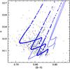 |
Fig. 1 Comparison between the observed HB of 47 Tuc (triangles) with synthetic CMDs calculated with ΔMRGB = 0.23 M⊙ and Y = 0.256, 0.270 and 0.286 (filled large circles), respectively, plus a simulation for ΔMRGB = 0.28 M⊙ and Y = 0.256 (dots). Two HB tracks corresponding to Y = 0.256, and masses M = 0.8 and 0.9 M⊙ (corresponding to ΔMRGB = 0.12 M⊙ and 0.02 M⊙, respectively) are shown as solid lines. All the tracks and synthetic CMDs are shifted by E(B − V) = 0.024 and (m − M)V = 13.40 (see text for details). |
Figure 1 displays a first test that shows clearly the need for a substantial mass loss and a range of initial Y values to match the location and morphology of the cluster HB. The three narrow synthetic sequences in the figure (filled circles) that overlap with the observed CMD were calculated for Y = 0.256 (the normal initial He for the chosen initial metallicity according to the ΔY/ ΔZ ~ 1.4 ratio employed in the BaSTI calculations, and a cosmological Y = 0.245) 0.270, and 0.286, respectively, ΔMRGB = 0.23, and a negligible Gaussian spread σ(ΔMRGB) = 0.001. The synthetic sequences were shifted in colour by applying the reference reddening E(B − V) = 0.024 and in magnitude by adding an apparent distance modulus (m − M)V = 13.40. This distance modulus is consistent with the estimates (m − M)V = 13.35 ± 0.08 (Thompson et al. 2010) and (m − M)V = 13.40 ± 0.07 (Kaluzny et al. 2007) from two eclipsing binaries in the cluster and has been chosen to match the bottom-right end of the observed HB with models calculated with the normal initial He.
The increase of initial He abundance at fixed mass loss moves the synthetic stars towards bluer colours and brighter magnitudes. This progressive shift in colours and magnitudes plus the increased extension of the blue loops in the synthetic populations reproduce well the wedge-shaped observed HB. For the reference age and metal composition, ΔMRGB = 0.23 M⊙ produces HB masses equal to 0.69, 0.66, and 0.63 M⊙ for Y = 0.256, 0.270, and 0.286, respectively (see also a similar discussion in Gratton et al. 2013). On the other hand, synthetic stars with Y = 0.256 and increased ΔMRGB = 0.28 M⊙ (dots) are displaced towards bluer colours but fainter magnitudes, confirming that the morphology of the cluster HB is driven by a range of Y rather than ΔMRGB.
We have shown also HB tracks for Y = 0.256 and masses equal to 0.8 and 0.9 M⊙ (in order of increasing colour and decreasing magnitude) that correspond to ΔMRGB = 0.12 M⊙ and 0.02 M⊙, respectively. These tracks are beyond the red edge of the observed HB and no variation of the adopted distance modulus can enforce an overlap with the data.
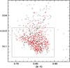 |
Fig. 2 Our baseline synthetic model for 47 Tuc HB (filled circles) compared to the observed HB (open triangles). The number of observed and synthetic stars within the box enclosing the observed HB is the same (see text for details). |
A full synthetic HB compared to the observed HB is shown in Fig. 2. For this complete simulation we had to assume a statistical distribution for the initial He abundances, which for simplicity we considered to be uniform. The range of Y values spans the interval 0.256−0.286 (Ymin = 0.256 and ΔY = 0.03) and ΔMRGB = 0.23 M⊙ as in Fig. 1 with a very small Gaussian spread of 0.005 M⊙. Photometric errors were assumed to be Gaussian with a mean value equal to 0.002 mag in both B and V magnitudes, as obtained from the photometric data. We restrict our comparison to the objects within the box highlighted in the CMD; the precise choice of the boundaries of the box is not crucial. The simulation contains a much larger number of stars than observed to minimize the Poisson error on the synthetic star counts, but for the sake of clarity we show a subset of synthetic objects that matches the number of observed stars. We considered the match to be satisfactory when the observed mean magnitude (⟨ V ⟩ HB = 14.07) and colour (⟨ (B − V)HB ⟩ = 0.80), plus the associated 1σ dispersions (0.04 mag in both cases) are reproduced within less than 0.005 mag, and the overall shape of the observed star counts as a function of both (B − V) and V is well reproduced. The mean (B − V) colour is matched for the assumed reddening E(B − V) = 0.024, and a distance modulus (m − M)V = 13.40 allows us to match the observed mean V magnitude as well.
Figure 3 shows the resulting histograms of observed and synthetic star counts as a function of V and (B − V); star counts from the synthetic CMD are rescaled to match the observed total number of HB stars. The agreement looks very good even with these simple assumptions about mass loss and He distribution.
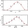 |
Fig. 3 Comparisons of synthetic (solid line) and observed (filled circles) star counts with Poisson error bars in V-magnitude (top panel: bin size equal to 0.04 mag) and (B − V) colour (bottom panel: bin size equal to 0.02 mag) bins, obtained from the data in Fig. 2 (see text for details). |
Figure 4 indicates mass and Y distributions as a function of the colour of the synthetic stars shown in Fig. 2. There is an obvious correlation with (B − V) for both mass and Y, as expected from the constant ΔMRGB (irrespective of Y) and very small σ(ΔMRGB) assumed in the simulation, which is blurred by the blue loops of the HB tracks (see Fig. 1). This is clear from the top panel, which shows how stars with a fixed mass are distributed over a large range of colours. Redder stars on the ZAHB are on average more massive and less He enriched than bluer objects; the typical mass for the stars with normal Y = 0.256 is ~0.69 M⊙ and decreases to ~0.63 M⊙ for Y = 0.286. The average mass along the synthetic HB is equal to 0.66 M⊙ with a 1σ dispersion of 0.017 M⊙. The exact values of these two quantities depend on the assumed distribution of initial Y, but obviously the mean mass cannot be outside the range 0.63−0.69 M⊙. A general trend of increasing Y with decreasing colour is also fully consistent with the observed trend of increasing Na towards bluer colours along the cluster HB (see Gratton et al. 2013).
We could have tried to enforce a priori the constraint of perfect statistical agreement between the theoretical and observed star counts. However, a perfect fit rests on the precise knowledge of the statistical distribution of ΔMRGB and the initial Y among the cluster stars. Owing to the current lack of firm theoretical and empirical guidance, this distribution may be extremely complicated and/or discontinuous. The constraints imposed on the matching synthetic HB are however sufficient to put strong constraints on ΔMRGB, which is the main parameter discussed in this work, and the range of initial Y, which determines the region of the CMD covered by the observed HB.
In fact, only the observed shape of the HB enables a good determination of both the ΔMRGB and Y range, when E(B − V), age and initial chemical composition are fixed, as can already be inferred from Fig. 1. In greater detail, Fig. 5 shows how changing these two parameters affects the shape and location of the synthetic HB. Variations of ΔMRGB around the reference value, keeping the reference Y distribution fixed, move the location of the synthetic HB along the direction from the top right corner of the CMD to the bottom left corner. At the same time, the HB gets compressed when ΔMRGB is reduced (shorter loops in the CMD of the HB tracks of larger mass) and stretched when ΔMRGB is increased. No change in the cluster distance modulus can bring into agreement any of these two synthetic CMDs with the observed HB. Variations of ΔY, keeping the reference ΔMRGB unchanged, stretch or compress the synthetic HB along the direction from the top left corner of the CMD to the bottom right corner. Also, in this case, variations of the cluster distance modulus do not compensate for the change of Y distribution.
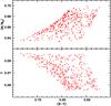 |
Fig. 4 Distribution of stellar mass (top panel) and initial Y values (bottom panel) as a function of the colour (B − V) for the stars in the synthetic CMD shown in Fig. 2. |
A decrease of ΔY to 0.025 and variations of ΔMRGB within less than 0.01 M⊙ do still allow a satisfactory fit to the observed HB, according to the criteria described above, but larger variations are clearly ruled out because the resulting synthetic HB would clearly have a different shape than observed. Values of ΔMRGB below 0.20 M⊙ are totally incompatible with the observed HB morphology and location in the CMD.
We also experimented with a mass loss that is linearly dependent on the initial Y distribution. Considering ΔMRGB = 0.23 M⊙ for the population with Ymin, a synthetic HB with ΔY = 0.03, and ΔMRGB increasing at most as 0.5 × ΔY provides a fit to the observations of comparable quality as the baseline simulation. This implies ΔMRGB is higher by just 0.015 M⊙ for the most He-rich component. Experiments with ΔMRGB decreasing with Y show that, at most, ΔMRGB can decrease as 0.15 × ΔY, implying a negligible decrease of the RGB mass loss as a function of Y.
As an additional test, we calculated a synthetic HB by considering the reference ΔMRGB = 0.230 ± 0.005 (Gaussian spread) for all Y, but with a different distribution of initial He abundances. We considered, in this case, 70% of the stars with a Gaussian distribution of initial Y characterized by mean value ⟨ Y ⟩ = 0.275 and spread σ(Y) = 0.007, and the remaining 30% with a very narrow Gaussian distribution with ⟨ Y ⟩ = 0.258 and spread σ(Y) = 0.0008. This choice stems from the results by Milone et al. (2012), who found a bimodal MS for this cluster, corresponding to ~0.02 difference in initial Y. The adopted distribution in our simulations has a difference of ~0.02 between the mean values of the two Gaussians and a total range ΔY = 0.03 that is needed to cover the V − (B − V) region occupied by observed HB completely. The 70/30 ratio again comes from the Milone et al. (2012) analysis of the number ratio between the two populations of different initial He as a function of the distance from the cluster centre. For the same distance modulus of our reference simulation, mean V and mean (B − V) of the observed HB are again matched within 0.01 mag, although star counts as a function of colour and magnitude are slightly less well reproduced.
The main point of this simulation is that a change of the initial Y distribution of the HB stars does not affect the ΔMRGB required to match the CMD location of the observed HB.
3. Analysis of the uncertainties
In the previous section we found that for the adopted reference [Fe/H] = −0.7, [α/Fe] = 0.4, E(B − V) = 0.024, t = 11.5 Gyr, our synthetic HB simulations require that RGB stars lose ΔMRGB = 0.23 M⊙ (and have a range of initial He abundances ΔY = 0.03) to match the observed location and morphology of the HB, corresponding to stellar masses in the range 0.63−0.69 M⊙. This value of ΔMRGB (and ΔY) is broadly in line with previous results based on synthetic HB modelling (di Criscienzo et al. 2010; Gratton et al. 2013), but in total disagreement with the conclusions by Heyl et al. (2015a) about RGB mass loss, based on cluster dynamics. The Heyl et al. (2015a) results specifically exclude HB masses of the order of 0.65 M⊙. In the following we discuss quantitatively how our reference estimate of ΔMRGB may be affected by a series of observational and theoretical uncertainties.
3.1. Cluster reddening, age, and chemical composition
The first obvious source of systematics is related to the range of reddening, chemical composition, and age estimates found in the literature. We analyzed these effects by varying one parameter at a time. In all these cases the value of ΔY required to reproduce the observations is unchanged compared to the baseline case.
Increasing E(B − V) (our baseline simulation has employed the lowest estimate of cluster reddening) tends to increase ΔMRGB. For example, assuming the widely employed value E(B − V) = 0.04, we obtain ΔMRGB = 0.24 M⊙, whilst we obtain ΔMRGB = 0.26 M⊙ for the upper limit E(B − V) = 0.055; that is we need lower masses to match the observed HB. As already mentioned, Marino et al. (2016) determined star-to-star variations around the mean reddening by at most −0.007 mag and +0.009 mag, respectively with mean variations that are smaller than these extreme values. This amount of differential reddening hardly affects the value of ΔMRGB, as detailed below.
To maximize this effect, we assume that the stars at the red edge of the observed HB all have a reddening that is 0.007 mag lower than the mean value. To compare with theory, their colours should then be increased by 0.007 mag, and their V magnitudes increased by ~0.02 mag, to reduce the observed HB to a single value of E(B − V), causing a decrease of ΔMRGB by just ~0.01 M⊙ in this extreme case. At the same time, assuming all stars along the blue edge of the wedge have a reddening 0.009 mag that is higher than the mean value, their colours should be decreased by the same amount and their V magnitudes also decreased by ~0.03 mag. This would require a negligible increase of ΔY and ΔMRGB increasing with Y as 0.6 ×ΔY.
As for the age, a variation by ±1 Gyr around the reference value causes a change of the RGB progenitor mass by about ±0.02 (lower mass for increasing age). The best-fit synthetic HB requires the same HB mass distribution as the baseline case, but ΔMRGB varies by about ±0.02 (decreased when the age increases) because of the change of the RGB progenitor mass.
We then considered the range of [Fe/H] estimates [Fe/H] = − 0.7 ± 0.1. Increasing [Fe/H] of the models tends to increase ΔMRGB for two reasons. First, because at fixed age the RGB progenitor mass increases by ~0.01 M⊙ for a 0.1 dex increase of [Fe/H] due to longer evolutionary timescales at fixed mass; second, HB tracks are redder so that for a fixed reddening, lower HB masses are required to match the observed HB location. If we consider [Fe/H] = − 0.6 –the approximate upper limit of the spectroscopic determinations, keeping everything else unchanged, the best-fit synthetic HB model has ΔY = 0.03, ΔMRGB = 0.28 M⊙, and (m − M)V = 13.35. When employing the approximate lower limit [Fe/H] = − 0.8, after interpolation in metallicity amongst the grid of BaSTI models, we obtain a best match for ΔY = 0.03, ΔMRGB=0.18 M⊙, and (m − M)V = 13.47. In these cases the mean mass of the synthetic HB stars varies by ~0.03 M⊙ (increases when [Fe/H] decreases) around the mean value of the baseline simulation.
If we decrease [α/Fe] from 0.4 dex to 0.3 dex, keeping [Fe/H] and all other parameters unchanged, after interpolations amongst our models we found that ΔMRGB decreases by just 0.01−0.02 M⊙ and (m − M)V increases by ~0.02 mag compared to our baseline simulation. The HB mean mass changes by less than the ΔMRGB because of the corresponding variation of the RGB progenitor mass, as for the case of changing [Fe/H]).
To summarize, variations of the cluster chemical composition, age, and reddening do not change the ΔMRGB much and, in particular, the typical HB stellar mass, compared to the results of the baseline simulation. In the following we discuss whether considering a number of uncertainties in the theoretical models can help solve or at least minimize the disagreement with inferences from cluster dynamics.
3.2. Bolometric corrections and colour transformations
To compare the output of stellar evolution calculations (L and Teff) with observed CMDs, the use of bolometric corrections (BCs) and colour-Teff relationships is essential. One way to proceed is to calculate grids of model atmospheres and synthetic spectra that are integrated under the appropriate filter transmission functions to get fluxes in a given passband, which are then suitably normalized to calculate BCs and colours (see e.g. Girardi et al. 2002; Casagrande & VandenBerg 2014, and references therein). Our adopted set of models employs theoretical BCs and colours calculated from ATLAS9 model atmospheres and spectra (see Pietrinferni et al. 2004, 2006, for details). We also tested the results from PHOENIX model atmosphere calculations employed by the Dartmouth stellar model library (Dotter et al. 2008), and found that at the relevant metallicities the HB tracks become systematically redder than with ATLAS9 results. This shift would cause lower HB masses from synthetic HB modelling, hence higher ΔMRGB at fixed age, reddening, and chemical composition.
An alternative approach is to employ empirical or semi-empirical results, when available. Worthey & Lee (2011) recently presented essentially empirical BCs and colour-Teff relationships in various broadband filters based on a collection of photometry for stars with known [Fe/H].
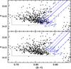 |
Fig. 6 HB evolutionary tracks for 0.7 (top panel) and 0.8 M⊙ (bottom panel), [Fe/H] = −0.7, [α/Fe] = 0.4, Y = 0.256 HB models shifted by E(B − V) = 0.024 and (m − M)V = 13.40, compared to the cluster HB. The dotted lines indicate BaSTI tracks with the adopted BaSTI BCs, and colour transformations, while the solid lines show the same tracks but employing the empirical Worthey & Lee (2011) BCs and colours. Dashed lines in each panel indicate the brightest and bluest, and the faintest and reddest extremes of the error range associated with Worthey & Lee (2011) transformations, respectively. |
Figure 6 shows representative 0.7 M⊙ and 0.8 M⊙ HB tracks with our adopted reference chemical composition and Y = 0.256, shifted by E(B − V) = 0.024 and (m − M)V = 13.40 as in our baseline simulation. The same tracks are displayed after applying BCs and colour transformations from Worthey & Lee (2011), using the routine provided by the authors. This routine also gives the errors associated with the computed BCs and colours, and we show in the figure the brightest/bluest and faintest/reddest limits of the area covered by these error bars, which are of about 0.05 mag in BCV and ~0.02 mag in (B − V).
It is clear from the figure that these transformations make the tracks redder (and very slightly fainter) than the reference BaSTI models, but within the empirical error bars ATLAS9 transformations (adopted in the BaSTI library) are consistent with Worthey & Lee (2011) results. There is not much room for a substantial increase of the typical HB mass when considering these empirical results. Masses above ~0.7 M⊙ along the HB are still clearly excluded.
To get more quantitative results, we calculated synthetic HB models for the reference chemical composition and reddening using Worthey & Lee (2011) results. We found a best match to the observed HB for ΔMRGB = 0.24 M⊙, which is very close to the result of our baseline simulation of Sect. 2, (m − M)V = 13.38; all of the other parameters are the same as in our reference simulation of Sect. 2. By employing the bluest colours allowed by the error bars on Worthey & Lee (2011) results to minimize the value of ΔMRGB and the HB masses needed by the HB simulations, we obtained ΔMRGB = 0.22 M⊙, and a mean HB mass equal to ~0.67 M⊙. Considering also the errors on BCV would simply shift the synthetic HB vertically by ±0.05 mag, implying an adjustment of the derived (m − M)V by the same amount, that is still within the errors of the eclipsing binary distance estimates.
3.3. Model calculation, input physics
Before the start of the HB phase, GC stars go through the violent core helium flash at the tip of the RGB. Until recently, only few calculations were able to calculate the evolution of stellar models through this event, and traditionally HB models (including the BaSTI models employed in our analysis) were computed by starting new sequences on the HB, where the initial structure is taken from that at the tip of the RGB. The underlying assumption of such methods, which are consistent with the results of stellar evolution calculations that follow the helium flash evolution, is that during the helium flash the internal (and surface) chemical structure is not altered significantly, apart from a small percentage of C produced in the He-core during the flash.
The technique employed in BaSTI models (denoted as Method 2 in the work by Serenelli & Weiss 2005) envisages that a model at the beginning of the core helium flash is employed as the starting model for the ZAHB calculation. The core mass and chemical profile of the initial pre-flash configuration are kept unchanged. The total mass of the ZAHB model is either preserved or reduced (to produce a set of ZAHB models of varying total mass) by rescaling the envelope mass. The new model on the ZAHB is then converged and relaxed for a certain amount of time (typically 1 Myr) to attain CNO equilibrium in the H-burning shell (see e.g. Cassisi & Salaris 2013) before being identified as the new ZAHB model. A 5% mass fraction of carbon is added to the He-core composition, guided by requirement that the energy needed for the expansion of the degenerate helium core must come from helium burning (Iben & Rood 1970).
VandenBerg et al. (2000) and, in greater detail Piersanti et al. (2004) and Serenelli & Weiss (2005), compared the ZAHB location and HB evolution of models whose RGB progenitor evolution was properly followed through the He-flash with results from our method described before. Especially for red HB models, as in the case of 47 Tuc HB, differences in Teff, L and time evolution turned out to be negligible.
As additional potential sources of uncertainty in the determination of ΔMRGB employing synthetic HB modelling, we considered the effect of uncertainties in the current input physics adopted in stellar model calculations. We considered first the effect on the He-core mass at the He-flash and how this affects the HB tracks, and then the effect on the HB evolution at fixed core mass.
Since the calculation of the BaSTI model database, two relevant physics inputs, i.e. the  reaction rate and the electron conduction opacities, have been the subjects of revised and improved determinations. The recent Cassisi et al. (2007) calculations of electron conduction opacities, larger than the Potekhin (1999) results used in the BaSTI calculations, cause a variation of the He-core mass at the He-flash (ΔMHec) by −0.006 M⊙, compared to our adopted HB models. On the other hand, the new Formicola et al. (2004) tabulations of the reaction rate, which is lower by a factor ~2 than the Angulo et al. (1999) rate used in our adopted model, induce an increase ΔMHec ~ 0.0025 M⊙ compared to the BaSTI calculations. The combined effect is a minor change ΔMHec ~ − 0.0035 M⊙ compared to the BaSTI models.
In addition, Valle et al. (2013) determined ΔMHec due to realistic uncertainties in the Formicola et al. (2004) reaction rate (±10%), the Cassisi et al. (2007) electron conduction opacities (±5%), plus the  (±3%) and 3α (±20%) reaction rates, neutrino emission rates (±4%), and the radiative opacities (±15%) used in the BaSTI models. If we simply add together the effect of these uncertainties plus the systematic effect of including fully efficient atomic diffusion in the pre-HB calculations4 that increase MHec by ~0.004 M⊙ (see Table 7.2 in Cassisi & Salaris 2013 and the ΔMHec ~ − 0.0035 M⊙ discussed before), we obtain a (conservative) variation ΔMHec ~ ± 0.01 M⊙ around the value obtained from the BaSTI calculations.
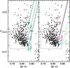 |
Fig. 7 As Fig. 6 but showing for the 0.8 M⊙ standard BaSTI track (solid line in both panels), the effect of changing the He-core mass at the He-flash by ±0.02 M⊙ (dashed lines in the left panel), the amount of He dredged to the surface by the first dredge up by δYFDU = ± 0.02 (dash-dotted lines in the left panel), the |
The left panel of Fig. 7 shows the effect of ΔMHec = ± 0.02 M⊙ on a 0.8 M⊙ HB track for the reference chemical composition Y = 0.256, [Fe/H] = − 0.7 and [α/Fe] = 0.4. To calculate this track, we varied the He-core mass by ±0.02 M⊙ around the value provided by the BaSTI models (MHec = 0.48 M⊙) and recalculated the HB evolution, as everything else was kept fixed. This variation is even larger than the estimates discussed before and takes two additional factors into account. First, there is a possible extra increase of MHec owing to the effect of rotation, as originally discussed by Castellani & Tornambe (1981) and Lee et al. (1994) in the context of synthetic HB modelling. Second, there is a potential additional decrease by ~0.008 M⊙ owing to the use of weak screening in the He-core during the whole RGB evolution, instead of the transition to intermediate and strong screening when appropriate, following the treatment by Graboske et al. (1973) as implemented in the BaSTI calculations.
It is clear from the figure that the expected shift in magnitude of the tracks (higher MHec corresponds to higher luminosity) is not accompanied by any major shift in colour. The ZAHB location is only very slightly redder for the lower core mass model and bluer for the higher core mass model and the extension of the loops in the CMD is only slightly altered. It may seem puzzling that such a large variation of MHec hardly affects the tracks. In fact HB tracks of a given total mass are generally sensitive to small variations of the He-core mass at the flash because of the changed efficiency of the H-burning shell due to the corresponding variation of the mass of the H-rich envelope. However, at this metallicity and for massive HB models, the efficiency of the burning shell is only weakly altered even by a ±0.02 M⊙ change of MHec because this corresponds to just a small percentage variation of the mass thickness of the envelope.
The same figure also shows the effect of arbitrarily altering the efficiency of the first dredge-up on the same 0.8 M⊙ HB track, keeping everything else unchanged. Our adopted BaSTI models predict an increase of the surface He mass fraction by 0.02 for the cluster RGB stars. This increased He abundance in the envelope impacts the efficiency of the H-burning shell during the HB phase. We tested a variation of the dredged-up He mass fraction δYFDU = ± 0.02 by recalculating HB models with this new envelope chemical abundance; the resulting tracks are simply shifted in luminosity (higher for increasing He abundance), but their colour location is unchanged.
We then considered the HB evolution of the same 0.8 M⊙ HB track keeping MHec fixed and varying the most relevant inputs one at a time as follows: for example the radiative opacities by ± 5%, the reaction rate from the Angulo et al. (1999) tabulations used in our adopted BaSTI models to the most updated Formicola et al. (2004) tabulations; the superadiabatic convection mixing length parameter by δαMLT = − 0.15, compared to the solar calibrated value (αml, ⊙ = 2.01) of the BaSTI calculations (see right panel of Fig. 7); and the  reaction rate (doubled and halved, respectively, as shown in the left panel of Fig. 7).
As already mentioned, the Formicola et al. (2004) rate is about a factor of two lower than the Angulo et al. (1999) result, i.e. a variation much larger than the error associated with this improved rate. Regarding the variation δαMLT = − 0.15 with respect to the solar calibrated value, this is what the fitting formulas by Magic et al. (2015), based on the results of a large grid of 3D radiation hydrodynamics simulations, predict for the surface gravity-effective temperature regime of the 0.8 M⊙ HB track and a metallicity [Fe/H] = − 0.5, which is close to the value adopted in our calculations. We consider this adopted δαMLT as a qualitative estimate of the uncertainty on the efficiency of superadiabatic convection in the envelope of red HB stars. Regardless of the precise estimate of δαMLT, Magic et al. (2015) simulations (a similar behaviour is also found in an analogous 3D hydro-calibration by Trampedach et al. 2014, at solar metallicity) predict that αMLT should decrease towards higher effective temperature and/or lower surface gravity compared to the solar values. As for the reaction rate, we consider both an increase and a decrease by a factor of two with respect to the reference rate adopted in the BaSTI calculations (Kunz et al. 2001), along the lines of the analysis by Gai (2013) regarding the current uncertainties on this reaction rate.
It is clear from the figure that the variation of the opacity, in which higher opacity corresponds to lower luminosities, and reaction rate essentially alter only the brightness of the model and not the colour, as for the case of varying MHec and YFDU. The variation of the reaction rate alters only very marginally the extension of the bluewards loop in the CMD (more extended loop for an increase of the reaction rate). The variation of the mixing length obviously affects the model colours, but the decrease of αMLT predicted by the hydro-simulations makes the model redder, thus decreasing the mass of the HB models, hence increasing the RGB mass loss, needed to match the observed HB5.
Finally, we considered the effect of the treatment of core mixing during the HB phase. As is well known and was discussed recently again by, for example Gabriel et al. (2014) and Constantino et al. (2015), the treatment of convective boundaries during core helium burning is still an open question in stellar evolution calculations and is handled in different ways by different stellar evolution codes. Recent advances in asteroseismic observations and techniques (Bossini et al. 2015; Constantino et al. 2015) are starting to add very direct observational constraints to the core mixing process during the central He-burning phase, which coupled with theoretical inferences and indications from star counts in Galactic globular clusters (see e.g. Caputo et al. 1989; Gabriel et al. 2014; Cassisi et al. 2003, and references therein), make a strong case for the core mixed region to be extended beyond the Schwarzschild border. Questions exist however about the treatment of this extended mixing. The details do not affect the ZAHB location of the models, but can potentially modify the extension of the loops in the CMD and have some relevance for the determination of the mass range of the cluster HB population.
Our adopted BaSTI HB models include semi-convection in the core (see Castellani et al. 1971b,a, 1985) with the suppression of the breathing pulses in the last phases of central He-burning with the technique by Caputo et al. (1989), following the observational constraints discussed by Cassisi et al. (2003). Constantino et al. (2016) calculated and compared HB models with different treatment of core mixing beyond the Schwarzschild border and, in their Fig. 7, they compare HB tracks for a 0.83 M⊙, [Fe/H] = −1, initial Y = 0.245; this comparison is not very different from the case discussed in this section. Tracks with two different types of overshooting and with semi-convection are almost indistinguishable; one of these types of overshooting, the maximal overshoot case, reproduces best the asteroseismic constraints, as discussed by Constantino et al. (2015).
As a conclusion, none of the items on the large list of uncertainties discussed in this section appears to be able to shift onto the observed HB substantially more massive HB tracks compared to the baseline simulation.
4. Discussion and conclusions
In the previous sections we investigated in detail the constraints posed by the CMD of HB stars on the RGB mass loss in the Galactic globular cluster 47 Tuc using synthetic HB modelling. We confirm the results by di Criscienzo et al. (2010) and Gratton et al. (2013) about the need for a range of initial He abundances (we find ΔY = 0.03) to reproduce the observed HB morphology properly. This abundance range is broadly consistent with the range inferred from the analysis of the cluster MS. For the values of age (11.5 Gyr), metal content ([Fe/H] = − 0.7 and [α/Fe] = 0.4), and reddening (E(B − V) = 0.024) adopted in our baseline simulation, a total mass loss of individual RGB stars ΔMRGB = 0.23 M⊙ (with a very small dispersion) independent of Y is required to reproduce the observed HB location and morphology. This value for ΔMRGB is consistent with the estimates by Origlia et al. (2007) from mid-IR photometry and the results by di Criscienzo et al. (2010) and Gratton et al. (2013) from similar synthetic HB modelling. The mean mass of the synthetic HB stars in this simulation is equal to 0.66 M⊙.
To assess the robustness of this estimate of ΔMRGB and the HB masses, we then considered several possible sources of uncertainty that could affect the HB modelling, stemming from uncertainties in both cluster parameters and model calculations. Uncertainties in the cluster reddening, age, and [Fe/H] have the largest effect on the derived ΔMRGB. Considering an age of 12.5 Gyr, which is approximately the upper limit consistent with current estimates, [Fe/H] = −0.8, which is the lower limit of spectroscopic estimates, and the lowest reddening estimate E(B − V) = 0.024 could potentially lead to ΔMRGB< 0.20 M⊙. Younger ages, higher metallicities, and reddenings, within the range of current estimates, can however increase the estimated ΔMRGB up to ~0.30 M⊙. A fraction of this range of ΔMRGB values is due to the variation of the RGB progenitor mass with age and initial chemical composition, so that the actual variation of the typical HB masses is smaller than the full range of ΔMRGB.
There is however the additional constraint posed by the observed colour of the RGB that can be considered. As we show in the following, this narrows the range of ΔMRGB and HB masses allowed by the analysis of the cluster CMD. The upper panel of Fig. 8 shows the synthetic CMDs of our baseline simulation described in Sect. 2 ([Fe/H] = − 0.7, [α/Fe] = 0.4, E(B − V) = 0.024, age t = 11.5 Gyr, ΔY = 0.03, ΔMRGB = 0.23 M⊙, (m − M)V = 13.40) together with the corresponding RGB isochrone (also from the BaSTI models, using the reference ATLAS9 transformations) compared to the cluster photometry in the magnitude range around the HB. Obviously the theoretical RGB is too red compared to the data; given that E(B − V) = 0.024 is the lowest reddening estimate, there is no room for shifting to the blue the position of the theoretical RGB, that is virtually insensitive to age and initial Y for the relevant age and He-abundance ranges. This implies that our adopted models with [Fe/H] = − 0.7 are inconsistent with the observations.
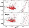 |
Fig. 8 As Fig. 2 but including also the observed and theoretical RGB sequences. The top panel displays the [Fe/H] = − 0.7 baseline simulation employing the BaSTI adopted BCs and colour transformations (ATLAS9). The bottom panel shows the result for the baseline simulation but employing the empirical Worthey & Lee (2011) BCs and colour transformations (solid line). The reddest and bluest limits of the RGB colours according to the errors on the Worthey & Lee (2011) transformations and BCs are displayed as dotted lines (see text for details). |
The lower panel of Fig. 8 refers to the best-match synthetic HB simulation when applying the Worthey & Lee (2011) transformations to our adopted BaSTI stellar models, keeping [Fe/H] = − 0.7, [α/Fe] = 0.4, E(B − V) = 0.024, t = 11.5 Gyr, as in the baseline simulation of the top panel. We derive in this case, as already discussed, ΔY = 0.03, ΔMRGB = 0.24 M⊙, (m − M)V = 13.38. The position of the RGB is again largely inconsistent with observations, even allowing for the errors on the Worthey & Lee (2011) BCs and colour transformations shown in the figure.
Figure 9 shows an analogous comparison, but for [Fe/H] = − 0.8 ([α/Fe] = 0.4), t = 11.5 Gyr. In the top panel, the case with the ATLAS9 BCs and colours, the theoretical RGB matches the average colour of the observed RGB for E(B − V) = 0.035, and the best-match synthetic HB has ΔY = 0.03, ΔMRGB = 0.19 M⊙, (m − M)V = 13.46. The average mass along the synthetic HB is in this case equal to 0.69 M⊙ with a 1σ dispersion of 0.017 M⊙, and a full range between ~0.65 M⊙ and ~0.73 M⊙.
The bottom panel indicates the case with the Worthey & Lee (2011) transformations for [Fe/H] = −0.8 ([α/Fe] = 0.4), t = 11.5 Gyr, E(B − V) = 0.035. The only way to match the observed RGB is to consider the bluest colours allowed by the errors on these empirical transformations, whilst for the HB the reference BCs and colour transformations provided by Worthey & Lee (2011) allow a match with observations for ΔY = 0.03, ΔMRGB = 0.19 M⊙, (m − M)V = 13.44, which is almost identical to the case with the ATLAS9 transformations.
One can speculate whether considering the bluest limit of Worthey & Lee (2011) colour transformations also for the HB models, might decrease ΔMRGB because the synthetic HB should then be made redder while keeping reddening, age, and chemical composition fixed. However, an increase of the HB masses, hence a decrease of ΔMRGB below ~0.19 M⊙, would cause a shift to the red of the HB, but also a change of the HB morphology that is inconsistent with the observations, as in the case discussed in the lower left panel of Fig. 5. With increasing HB mass, the loops in the CMD shrink and it is impossible to match simultaneously the vertical and horizontal thickness of the observed HB by changing the Y distribution.
In summary, the additional constraint posed by the colour of the RGB narrows down the possible range of [Fe/H], E(B − V) and ΔMRGB. A fit for the minimum estimate E(B − V) = 0.024 could, in principle, be achieved, at least with the ATLAS9 transformations, considering a slightly higher [Fe/H] of between ~−0.8 and ~−0.75 dex; however, this would keep ΔMRGB, and the evolving HB masses, roughly unchanged because of the compensating effects of increasing [Fe/H] and decreasing reddening, as discussed in the previous sections.
A firm estimate of the minimum RGB mass loss allowed by our modelling is therefore ΔMRGB ~ 0.17 M⊙ if we consider a cluster age of 12.5 Gyr that is approximately the upper limit of current estimates. The maximum ΔMRGB is equal to ~0.21 M⊙, for an age of 10.5 Gyr. The resulting mass distribution of the HB stars is in both cases between 0.65 M⊙ and 0.73 M⊙, which is the full range determined mainly by the range of initial Y abundances of the progenitors (ΔY = 0.03). The derived distance modulus is consistent with constraints from the observed cluster eclipsing binaries.
We can also compare ΔMRGB with the expected mass loss during the following AGB phase (ΔMAGB). In the simulation that minimizes ΔMRGB, the initial progenitor mass of the HB stars is equal to ~0.89 M⊙ for the Y = 0.254 population and ~0.84 M⊙ for the Y = 0.284 population. Assuming that the final WD mass is equal to ~0.53 M⊙ (Kalirai et al. 2009) irrespective of the initial Y, the mass to be shed by the cluster stars during the AGB phase ranges between ΔMAGB ~ 0.19 M⊙ for the Y = 0.254 population and ~0.14 M⊙ for the Y = 0.284 population. The value of ΔMRGB is therefore expected to be similar to the average ΔMAGB, whose precise value depends on the distribution of initial Y. For a flat Y distribution the average ΔMAGB is equal to ΔMRGB.
On the whole our detailed analysis confirms the discrepancy between information coming from cluster dynamics and CMD modelling of the HB. The lower limit for ΔMRGB allowed by the HB modelling is only slightly lower than the 0.20 M⊙ value excluded with high confidence by the Heyl et al. (2015a) analysis. The predicted mass distribution of HB stars is between ~0.65 M⊙ and ~0.73 M⊙ with mean values, which depend on the exact Y distribution, and are not much higher than 0.65 M⊙; this latter is excluded by the Heyl et al. (2015a) analysis. On the other hand, the RGB mass loss allowed by the HB modelling is consistent with ΔMRGB ~ 0.23 ± 0.07M⊙ estimated from the detection of their circumstellar envelopes by means of mid-IR photometry (Origlia et al. 2007).
A comparison between the results from these two techniques applied to other clusters is required to gain more insights into the origin of this apparently major disagreement between CMD and dynamical results.
Higher reddenings require a larger shift to the red of the HB models, hence a lower HB mass at a given colour and an increased amount of RGB mass loss to match the observed HB location.
Light element anti-correlations do not affect the bolometric corrections for MS stars in optical CMDs, as shown by Sbordone et al. (2011).
The BaSTI models neglect atomic diffusion.
Somewhat surprisingly, the V-band magnitude of the model with changed mixing length is also affected, although this is exclusively due to the bolometric corrections, which change because of the decrease of the model effective temperature.
Acknowledgments
We thank the referee for comments that pushed us to improve the analysis of Sect. 3.3. S.C. warmly thanks the financial support by PRIN-INAF2014 (PI: S. Cassisi) and the Economy and Competitiveness Ministry of the Kingdom of Spain (grant AYA2013-42781-P). A.P. acknowledges financial support by PRIN-INAF 2012 The M4 Core Project with Hubble Space Telescope (P.I.: L. Bedin).
References
- Angulo, C., Arnould, M., Rayet, M., et al. 1999, Nucl. Phys. A, 656, 3 [NASA ADS] [CrossRef] [Google Scholar]
- Bergbusch, P. A., & Stetson, P. B. 2009, AJ, 138, 1455 [NASA ADS] [CrossRef] [Google Scholar]
- Bossini, D., Miglio, A., Salaris, M., et al. 2015, MNRAS, 453, 2290 [NASA ADS] [CrossRef] [Google Scholar]
- Boyer, M. L., van Loon, J. T., McDonald, I., et al. 2010, ApJ, 711, L99 [NASA ADS] [CrossRef] [Google Scholar]
- Caputo, F., Chieffi, A., Tornambe, A., Castellani, V., & Pulone, L. 1989, ApJ, 340, 241 [NASA ADS] [CrossRef] [Google Scholar]
- Casagrande, L., & VandenBerg, D. A. 2014, MNRAS, 444, 392 [NASA ADS] [CrossRef] [MathSciNet] [Google Scholar]
- Cassisi, S., & Salaris, M. 2013, Old Stellar Populations: How to Study the Fossil Record of Galaxy Formation (Wiley-VCH) [Google Scholar]
- Cassisi, S., Salaris, M., & Irwin, A. W. 2003, ApJ, 588, 862 [NASA ADS] [CrossRef] [Google Scholar]
- Cassisi, S., Potekhin, A. Y., Pietrinferni, A., Catelan, M., & Salaris, M. 2007, ApJ, 661, 1094 [NASA ADS] [CrossRef] [Google Scholar]
- Cassisi, S., Mucciarelli, A., Pietrinferni, A., Salaris, M., & Ferguson, J. 2013, A&A, 554, A19 [EDP Sciences] [Google Scholar]
- Castellani, M., & Castellani, V. 1993, ApJ, 407, 649 [NASA ADS] [CrossRef] [Google Scholar]
- Castellani, V., & Tornambe, A. 1981, A&A, 96, 207 [NASA ADS] [Google Scholar]
- Castellani, V., Giannone, P., & Renzini, A. 1971a, Ap&SS, 10, 355 [NASA ADS] [CrossRef] [Google Scholar]
- Castellani, V., Giannone, P., & Renzini, A. 1971b, Ap&SS, 10, 340 [NASA ADS] [CrossRef] [Google Scholar]
- Castellani, V., Chieffi, A., Tornambe, A., & Pulone, L. 1985, ApJ, 296, 204 [NASA ADS] [CrossRef] [Google Scholar]
- Catelan, M. 1993, A&AS, 98, 547 [NASA ADS] [Google Scholar]
- Catelan, M., & de Freitas Pacheco, J. A. 1996, PASP, 108, 166 [NASA ADS] [CrossRef] [Google Scholar]
- Constantino, T., Campbell, S. W., Christensen-Dalsgaard, J., Lattanzio, J. C., & Stello, D. 2015, MNRAS, 452, 123 [NASA ADS] [CrossRef] [Google Scholar]
- Constantino, T., Campbell, S. W., Lattanzio, J. C., & van Duijneveldt, A. 2016, MNRAS, 456, 3866 [NASA ADS] [CrossRef] [Google Scholar]
- Cordero, M. J., Pilachowski, C. A., Johnson, C. I., et al. 2014, ApJ, 780, 94 [NASA ADS] [CrossRef] [Google Scholar]
- Dalessandro, E., Salaris, M., Ferraro, F. R., Mucciarelli, A., & Cassisi, S. 2013, MNRAS, 430, 459 [NASA ADS] [CrossRef] [Google Scholar]
- D’Antona, F., Caloi, V., Montalbán, J., Ventura, P., & Gratton, R. 2002, A&A, 395, 69 [NASA ADS] [CrossRef] [EDP Sciences] [Google Scholar]
- Decressin, T., Meynet, G., Charbonnel, C., Prantzos, N., & Ekström, S. 2007, A&A, 464, 1029 [NASA ADS] [CrossRef] [EDP Sciences] [Google Scholar]
- D’Ercole, A., D’Antona, F., Ventura, P., Vesperini, E., & McMillan, S. L. W. 2010, MNRAS, 407, 854 [NASA ADS] [CrossRef] [MathSciNet] [Google Scholar]
- di Criscienzo, M., Ventura, P., D’Antona, F., Milone, A., & Piotto, G. 2010, MNRAS, 408, 999 [NASA ADS] [CrossRef] [Google Scholar]
- Dorman, B., Vandenberg, D. A., & Laskarides, P. G. 1989, ApJ, 343, 750 [NASA ADS] [CrossRef] [Google Scholar]
- Dotter, A., Chaboyer, B., Jevremović, D., et al. 2008, ApJS, 178, 89 [NASA ADS] [CrossRef] [Google Scholar]
- Dotter, A., Sarajedini, A., Anderson, J., et al. 2010, ApJ, 708, 698 [NASA ADS] [CrossRef] [Google Scholar]
- Formicola, A., Imbriani, G., Costantini, H., et al. 2004, Phys. Lett. B, 591, 61 [NASA ADS] [CrossRef] [Google Scholar]
- Gabriel, M., Noels, A., Montalbán, J., & Miglio, A. 2014, A&A, 569, A63 [NASA ADS] [CrossRef] [EDP Sciences] [Google Scholar]
- Gai, M. 2013, Phys. Rev. C, 88, 062801 [Google Scholar]
- Girardi, L., Bertelli, G., Bressan, A., et al. 2002, A&A, 391, 195 [NASA ADS] [CrossRef] [EDP Sciences] [Google Scholar]
- Graboske, H. C., Dewitt, H. E., Grossman, A. S., & Cooper, M. S. 1973, ApJ, 181, 457 [NASA ADS] [CrossRef] [Google Scholar]
- Gratton, R. G., Fusi Pecci, F., Carretta, E., et al. 1997, ApJ, 491, 749 [NASA ADS] [CrossRef] [Google Scholar]
- Gratton, R. G., Bragaglia, A., Carretta, E., et al. 2003, A&A, 408, 529 [NASA ADS] [CrossRef] [EDP Sciences] [Google Scholar]
- Gratton, R., Sneden, C., & Carretta, E. 2004, ARA&A, 42, 385 [NASA ADS] [CrossRef] [Google Scholar]
- Gratton, R. G., Carretta, E., Bragaglia, A., Lucatello, S., & D’Orazi, V. 2010, A&A, 517, A81 [NASA ADS] [CrossRef] [EDP Sciences] [Google Scholar]
- Gratton, R. G., Lucatello, S., Sollima, A., et al. 2013, A&A, 549, A41 [NASA ADS] [CrossRef] [EDP Sciences] [Google Scholar]
- Groenewegen, M. A. T. 2012, A&A, 540, A32 [NASA ADS] [CrossRef] [EDP Sciences] [Google Scholar]
- Harris, W. E. 1996, AJ, 112, 1487 [NASA ADS] [CrossRef] [Google Scholar]
- Heyl, J., Kalirai, J., Richer, H. B., et al. 2015a, ApJ, 810, 127 [NASA ADS] [CrossRef] [Google Scholar]
- Heyl, J., Richer, H. B., Antolini, E., et al. 2015b, ApJ, 804, 53 [NASA ADS] [CrossRef] [Google Scholar]
- Iben, Jr., I., & Rood, R. T. 1970, ApJ, 161, 587 [NASA ADS] [CrossRef] [Google Scholar]
- Kalirai, J. S., Saul Davis, D., Richer, H. B., et al. 2009, ApJ, 705, 408 [NASA ADS] [CrossRef] [Google Scholar]
- Kaluzny, J., Thompson, I. B., Rucinski, S. M., et al. 2007, AJ, 134, 541 [NASA ADS] [CrossRef] [Google Scholar]
- Kunz, R., Jaeger, M., Mayer, A., et al. 2001, Phys. Rev. Lett., 86, 3244 [NASA ADS] [CrossRef] [MathSciNet] [PubMed] [Google Scholar]
- Lee, Y.-W., Demarque, P., & Zinn, R. 1990, ApJ, 350, 155 [NASA ADS] [CrossRef] [Google Scholar]
- Lee, Y.-W., Demarque, P., & Zinn, R. 1994, ApJ, 423, 248 [Google Scholar]
- Magic, Z., Weiss, A., & Asplund, M. 2015, A&A, 573, A89 [NASA ADS] [CrossRef] [EDP Sciences] [Google Scholar]
- Marino, A. F., Milone, A. P., Casagrande, L., et al. 2016, MNRAS, 459, 610 [NASA ADS] [CrossRef] [Google Scholar]
- Mauas, P. J. D., Cacciari, C., & Pasquini, L. 2006, A&A, 454, 609 [NASA ADS] [CrossRef] [EDP Sciences] [Google Scholar]
- McDonald, I., & Zijlstra, A. A. 2015, MNRAS, 448, 502 [NASA ADS] [CrossRef] [Google Scholar]
- Milone, A. P., Piotto, G., Bedin, L. R., et al. 2012, ApJ, 744, 58 [NASA ADS] [CrossRef] [Google Scholar]
- Milone, A. P., Marino, A. F., Piotto, G., et al. 2013, ApJ, 767, 120 [NASA ADS] [CrossRef] [Google Scholar]
- Milone, A. P., Marino, A. F., Dotter, A., et al. 2014, ApJ, 785, 21 [NASA ADS] [CrossRef] [Google Scholar]
- Momany, Y., Saviane, I., Smette, A., et al. 2012, A&A, 537, A2 [NASA ADS] [CrossRef] [EDP Sciences] [Google Scholar]
- Nardiello, D., Milone, A. P., Piotto, G., et al. 2015, A&A, 573, A70 [NASA ADS] [CrossRef] [EDP Sciences] [Google Scholar]
- Origlia, L., Rood, R. T., Fabbri, S., et al. 2007, ApJ, 667, L85 [NASA ADS] [CrossRef] [Google Scholar]
- Origlia, L., Rood, R. T., Fabbri, S., et al. 2010, ApJ, 718, 522 [NASA ADS] [CrossRef] [Google Scholar]
- Piersanti, L., Tornambé, A., & Castellani, V. 2004, MNRAS, 353, 243 [NASA ADS] [CrossRef] [Google Scholar]
- Pietrinferni, A., Cassisi, S., Salaris, M., & Castelli, F. 2004, ApJ, 612, 168 [NASA ADS] [CrossRef] [Google Scholar]
- Pietrinferni, A., Cassisi, S., Salaris, M., & Castelli, F. 2006, ApJ, 642, 797 [NASA ADS] [CrossRef] [Google Scholar]
- Pietrinferni, A., Cassisi, S., Salaris, M., Percival, S., & Ferguson, J. W. 2009, ApJ, 697, 275 [NASA ADS] [CrossRef] [Google Scholar]
- Piotto, G., Bedin, L. R., Anderson, J., et al. 2007, ApJ, 661, L53 [NASA ADS] [CrossRef] [Google Scholar]
- Potekhin, A. Y. 1999, A&A, 351, 787 [NASA ADS] [Google Scholar]
- Reimers, D. 1975, Mem. Soc. Roy. Sci. Liege, 8, 369 [Google Scholar]
- Rood, R. T. 1973, ApJ, 184, 815 [NASA ADS] [CrossRef] [Google Scholar]
- Salaris, M., & Weiss, A. 2002, A&A, 388, 492 [NASA ADS] [CrossRef] [EDP Sciences] [Google Scholar]
- Salaris, M., Riello, M., Cassisi, S., & Piotto, G. 2004, A&A, 420, 911 [NASA ADS] [CrossRef] [EDP Sciences] [Google Scholar]
- Salaris, M., Held, E. V., Ortolani, S., Gullieuszik, M., & Momany, Y. 2007, A&A, 476, 243 [NASA ADS] [CrossRef] [EDP Sciences] [Google Scholar]
- Sarajedini, A., Bedin, L. R., Chaboyer, B., et al. 2007, AJ, 133, 1658 [NASA ADS] [CrossRef] [Google Scholar]
- Sbordone, L., Salaris, M., Weiss, A., & Cassisi, S. 2011, A&A, 534, A9 [NASA ADS] [CrossRef] [EDP Sciences] [Google Scholar]
- Schlegel, D. J., Finkbeiner, D. P., & Davis, M. 1998, ApJ, 500, 525 [NASA ADS] [CrossRef] [Google Scholar]
- Schröder, K.-P., & Cuntz, M. 2005, ApJ, 630, L73 [NASA ADS] [CrossRef] [Google Scholar]
- Serenelli, A., & Weiss, A. 2005, A&A, 442, 1041 [NASA ADS] [CrossRef] [EDP Sciences] [Google Scholar]
- Thompson, I. B., Kaluzny, J., Rucinski, S. M., et al. 2010, AJ, 139, 329 [NASA ADS] [CrossRef] [Google Scholar]
- Trampedach, R., Stein, R. F., Christensen-Dalsgaard, J., Nordlund, Å., & Asplund, M. 2014, MNRAS, 445, 4366 [NASA ADS] [CrossRef] [Google Scholar]
- Valle, G., Dell’Omodarme, M., Prada Moroni, P. G., & Degl’Innocenti, S. 2013, A&A, 549, A50 [NASA ADS] [CrossRef] [EDP Sciences] [Google Scholar]
- VandenBerg, D. A., Swenson, F. J., Rogers, F. J., Iglesias, C. A., & Alexander, D. R. 2000, ApJ, 532, 430 [NASA ADS] [CrossRef] [Google Scholar]
- VandenBerg, D. A., Brogaard, K., Leaman, R., & Casagrande, L. 2013, ApJ, 775, 134 [NASA ADS] [CrossRef] [Google Scholar]
- Vieytes, M., Mauas, P., Cacciari, C., Origlia, L., & Pancino, E. 2011, A&A, 526, A4 [NASA ADS] [CrossRef] [EDP Sciences] [Google Scholar]
- Worthey, G., & Lee, H.-C. 2011, ApJS, 193, 1 [NASA ADS] [CrossRef] [EDP Sciences] [Google Scholar]
All Figures
|
Fig. 1 Comparison between the observed HB of 47 Tuc (triangles) with synthetic CMDs calculated with ΔMRGB = 0.23 M⊙ and Y = 0.256, 0.270 and 0.286 (filled large circles), respectively, plus a simulation for ΔMRGB = 0.28 M⊙ and Y = 0.256 (dots). Two HB tracks corresponding to Y = 0.256, and masses M = 0.8 and 0.9 M⊙ (corresponding to ΔMRGB = 0.12 M⊙ and 0.02 M⊙, respectively) are shown as solid lines. All the tracks and synthetic CMDs are shifted by E(B − V) = 0.024 and (m − M)V = 13.40 (see text for details). |
| In the text | |
|
Fig. 2 Our baseline synthetic model for 47 Tuc HB (filled circles) compared to the observed HB (open triangles). The number of observed and synthetic stars within the box enclosing the observed HB is the same (see text for details). |
| In the text | |
|
Fig. 3 Comparisons of synthetic (solid line) and observed (filled circles) star counts with Poisson error bars in V-magnitude (top panel: bin size equal to 0.04 mag) and (B − V) colour (bottom panel: bin size equal to 0.02 mag) bins, obtained from the data in Fig. 2 (see text for details). |
| In the text | |
|
Fig. 4 Distribution of stellar mass (top panel) and initial Y values (bottom panel) as a function of the colour (B − V) for the stars in the synthetic CMD shown in Fig. 2. |
| In the text | |
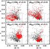 |
Fig. 5 As Fig. 2, but for the labelled values of ΔMRGB and ΔY (see text for details). |
| In the text | |
|
Fig. 6 HB evolutionary tracks for 0.7 (top panel) and 0.8 M⊙ (bottom panel), [Fe/H] = −0.7, [α/Fe] = 0.4, Y = 0.256 HB models shifted by E(B − V) = 0.024 and (m − M)V = 13.40, compared to the cluster HB. The dotted lines indicate BaSTI tracks with the adopted BaSTI BCs, and colour transformations, while the solid lines show the same tracks but employing the empirical Worthey & Lee (2011) BCs and colours. Dashed lines in each panel indicate the brightest and bluest, and the faintest and reddest extremes of the error range associated with Worthey & Lee (2011) transformations, respectively. |
| In the text | |
|
Fig. 7 As Fig. 6 but showing for the 0.8 M⊙ standard BaSTI track (solid line in both panels), the effect of changing the He-core mass at the He-flash by ±0.02 M⊙ (dashed lines in the left panel), the amount of He dredged to the surface by the first dredge up by δYFDU = ± 0.02 (dash-dotted lines in the left panel), the |
| In the text | |
|
Fig. 8 As Fig. 2 but including also the observed and theoretical RGB sequences. The top panel displays the [Fe/H] = − 0.7 baseline simulation employing the BaSTI adopted BCs and colour transformations (ATLAS9). The bottom panel shows the result for the baseline simulation but employing the empirical Worthey & Lee (2011) BCs and colour transformations (solid line). The reddest and bluest limits of the RGB colours according to the errors on the Worthey & Lee (2011) transformations and BCs are displayed as dotted lines (see text for details). |
| In the text | |
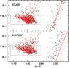 |
Fig. 9 As Fig. 8, but for simulations with [Fe/H] = −0.8 (see text for details). |
| In the text | |
Current usage metrics show cumulative count of Article Views (full-text article views including HTML views, PDF and ePub downloads, according to the available data) and Abstracts Views on Vision4Press platform.
Data correspond to usage on the plateform after 2015. The current usage metrics is available 48-96 hours after online publication and is updated daily on week days.
Initial download of the metrics may take a while.