A chemical model for the interstellar medium in galaxies

S. Bovino; T. Grassi; P. R. Capelo; D. R. G. Schleicher; R. Banerjee

doi:10.1051/0004-6361/201628158

Home

All issues

Volume 590 (June 2016)

A&A, 590 (2016) A15

Full HTML

Free Access

Issue		A&A Volume 590, June 2016


Article Number		A15
Number of page(s)		23
Section		Astrophysical processes
DOI		https://doi.org/10.1051/0004-6361/201628158
Published online		28 April 2016

A&A 590, A15 (2016)

A chemical model for the interstellar medium in galaxies

S. Bovino¹, T. Grassi², P. R. Capelo³, D. R. G. Schleicher⁴ and R. Banerjee¹

¹ Hamburger Sternwarte, Universität Hamburg, Gojenbergsweg 112, 21029 Hamburg, Germany
e-mail: stefano.bovino@uni-hamburg.de
² Centre for Star and Planet Formation, Niels Bohr Institute & Natural History Museum of Denmark, University of Copenhagen, Øster Voldgade 5–7, 1350 Copenhagen, Denmark
³ Center for Theoretical Astrophysics and Cosmology, Institute for Computational Science, University of Zurich, Winterthurerstrasse 190, 8057 Zürich, Switzerland
⁴ Departamento de Astronomía, Facultad Ciencias Físicas y Matemáticas, Universidad de Concepción, Av. Esteban Iturra s/n Barrio Universitario, Casilla 160, Concepción, Chile

Received: 19 January 2016
Accepted: 15 February 2016

Abstract

Aims. We present and test chemical models for three-dimensional hydrodynamical simulations of galaxies. We explore the effect of changing key parameters such as metallicity, radiation, and non-equilibrium versus equilibrium metal cooling approximations on the transition between the gas phases in the interstellar medium.

Methods. The microphysics was modelled by employing the public chemistry package KROME, and the chemical networks were tested to work in a wide range of densities and temperatures. We describe a simple H/He network following the formation of H₂ and a more sophisticated network that includes metals. Photochemistry, thermal processes, and different prescriptions for the H₂ catalysis on dust are presented and tested within a one-zone framework. The resulting network is made publicly available on the KROME webpage.

Results. We find that employing an accurate treatment of the dust-related processes induces a faster HI–H₂ transition. In addition, we show when the equilibrium assumption for metal cooling holds and how a non-equilibrium approach affects the thermal evolution of the gas and the HII–HI transition.

Conclusions. These models can be employed in any hydrodynamical code via an interface to KROME and can be applied to different problems including isolated galaxies, cosmological simulations of galaxy formation and evolution, supernova explosions in molecular clouds, and the modelling of star-forming regions. The metal network can be used for a comparison with observational data of CII 158 μm emission both for high-redshift and for local galaxies.

Key words: astrochemistry / molecular processes / galaxies: ISM / methods: numerical / evolution

© ESO, 2016

1. Introduction

To follow the formation and evolution of galaxies is a computational challenge because many non-linear processes have to be taken into account. For instance, magnetic fields, turbulence, heating and cooling, star formation, feedback, and supermassive black holes are some of the most important ingredients that make the galactic environment diverse and very complex. Furthermore, the involved spatial and temporal scales span a wide range, and it is difficult to explore the dynamics and the physics on all the relevant scales without introducing subgrid-scale models. These are mainly oriented towards describing small-scale phenomena, such as star formation and stellar feedback (McKee & Ostriker 1977; Offner et al. 2009; Braun & Schmidt 2012; Federrath et al. 2014; Hopkins et al. 2014; Semenov et al. 2015) and properties of turbulence (Schmidt & Federrath 2011; Grete et al. 2015), and are based on observational constraints. In particular, the star formation process, i.e. the conversion of cold gas into stars, is typically tuned according to the Kennicutt-Schmidt (KS) relation (Schmidt 1959, 1963; Kennicutt 1989, 1998), which connects the star formation rate (SFR) to the total gas surface density Σ_gas. Since the work by Wong & Blitz (2002), a tight linear correlation between SFR and the H₂ content (Σ_H₂) has been indicated, and it has been shown that the traditional KS relation can break down in the HI regions of galaxies (Bigiel et al. 2008, 2010; Leroy et al. 2008; Schruba et al. 2011).

The lack of an electric dipole moment makes the H₂ line transitions very weak and difficult to be observed, so that CO has been widely used as a good tracer of the cold phase (see Carilli & Walter 2013, for a recent review). However, Krumholz (2012) shows that, at metallicities below a few per cent of solar metallicity, star formation could take place in HI-dominated regions, and the argument that correlates the star formation to molecular gas breaks down. In addition, a universal turbulence-regulated star formation law has also been proposed by different authors (e.g. Krumholz et al. 2012; Federrath 2013; Salim et al. 2015). It is, moreover, important to highlight recent observations of the bright CII 158 μm transition both in high-redshift galaxies with ALMA (Maiolino et al. 2015) and in quasars with IRAM (Bañados et al. 2015), as well as in local galaxies with HERSCHEL (e.g. Pineda et al. 2014), which provide an alternative path for measuring the SFR in the different gas phases of the galaxy. It is then very important to follow the evolution of the gas between the different phases and to include a proper chemical model that can track the time-dependent H₂ and/or CII evolution in simulations that aim to study the correlation between SFR and the different gas components.

Analytical and semi-analytical models, some of which are based on equilibrium chemistry, have been proposed to track the formation of molecular hydrogen in three-dimensional (3D) hydrodynamic simulations of galaxies (Krumholz et al. 2008; Kuhlen et al. 2012; Braun & Schmidt 2012; Somerville et al. 2015). A model that follows the non-equilibrium H₂ evolution, coupled with a radiative transfer algorithm, and a simple prescription for metal-line cooling, has been reported by Gnedin et al. (2009), who also linked the SFR directly to the H₂ density, performing simulations with the Adaptive Refinement Tree (ART) code. They included the most important paths for H₂ formation and destruction, i.e. photodissociation by UV Lyman-Werner photons, formation on dust, and gas phase formation via H and H⁻, and employed a clumping factor C_ρ to take the unresolved high density regions into account on small scales. This network was extended to a more detailed model that includes He-based species in a follow-up work (Gnedin & Kravtsov 2011) and employed in realistic cosmological simulations of a galaxy at redshift z = 4.

The minimal chemical model by Gnedin et al. (2009) has been implemented in cosmological simulations of galaxies performed with the hydrodynamic codes GASOLINE (Christensen et al. 2012) and RAMSES (Tomassetti et al. 2015), which also directly connected the SFR to the H₂ content. Pelupessy & Papadopoulos (2009) additionally explored an H₂-regulated star formation recipe performing cosmological simulations with a time-dependent approach to follow the HI-H₂ transition. However, whether the SFR should be directly proportional to the H₂ content (ρ_H₂) or to the total gas density (ρ_gas) is still a matter of ongoing debate, and more observational constraints are needed.

In a recent paper, Hu et al. (2015) discuss the connection of star formation to the HI and H₂ gas phases, and the way it is affected by changing the UV radiation strength, employing a non-equilibrium model for the chemistry. Their chemical network is based on six species, of which only three are followed time-dependently (H₂, H⁺, and CO), and it includes the most important heating and cooling processes. The results from high-resolution hydrodynamical simulations for an isolated dwarf galaxy performed with the smoothed-particle hydrodynamics code GADGET-3, showed that the dust-to-gas ratio and the radiation background mostly affect the H₂ formation rate instead of the SFR and that the cold phase is dominated by HI.

Richings et al. (2014) present a complex CO chemical network and performed hydrodynamical simulations of an isolated galaxy assuming a static potential for the dark matter (Richings & Schaye 2016). Many ingredients, including cosmic rays and X-rays, have been included, and results for different metallicities and UV background strength were discussed.

More recently, a strong effort has been made to settle a code comparison of different hydrodynamics codes on galaxy simulations, which share common physics and analysis tools (Kim et al. 2014). However, the AGORA project mainly aims at studying the atomic gas phase and at understanding whether the differences produced by the different hydrodynamic codes can be attributed to the employed physics or the different numerical techniques used to solve the hydrodynamical equations.

In this paper we present a set of chemical models, publicly released via the KROME package¹, which can be used to study the transitions between the different gas phases in galaxy simulations with different degrees of accuracy. We provide a method for non-equilibrium H₂ prescription, and a more complex network including metals that can be employed to follow the evolution of CII at different metallicities.

The paper is organized as follows. In Sect. 2, we present the most important physical ingredients that regulate the thermal and chemical evolution of the gas and their computational implementation in the public code KROME. In Sect. 3, we test the chemical networks and the microphysics employing a simple one-zone collapse framework. We explore four different models under different conditions, i.e. changing the metallicity, the chemical initial conditions, the radiation background strength, and the dust-related physics. We finally provide our conclusions in Sect. 4.

2. Microphysics

2.1. The KROME package

The microphysics and the chemical networks described in the following sections were developed within the publicly available astrochemistry package KROME (Grassi et al. 2014). It consists of a python module that, given a chemical network and a series of physics-related options, generates the code to solve a system of coupled ordinary differential equations (ODEs) that follow the thermo-chemical evolution of the gas. KROME includes precompiled networks and different modules for the microphysics, such as cooling/heating functions, photochemistry, and a dust module for cooling and molecule catalysis. Since its release, KROME has been employed to study a variety of astrophysical problems, such as the formation of supermassive black holes under UV radiation and in the presence of dust (Latif et al. 2014, 2015b,a), the collapse of low-metallicity minihaloes (Bovino et al. 2014a), formation of primordial stars (Bovino et al. 2014b), the chemical evolution of self-gravitating primordial disks (Schleicher et al. 2016), the formation of the first galaxies (Prieto et al. 2015), the formation of very massive stars (Katz et al. 2015), and star-forming filaments in molecular clouds (Seifried & Walch 2015).

A wide range of physical and chemical conditions has been explored by employing KROME with different hydrodynamical codes (e.g. ENZO, RAMSES, and FLASH) showing its flexibility. In addition, KROME employs the accurate and stable chemical solver DLSODES (Hindmarsh 1983), which is suitable for studying highly non-linear problems where the spatial and temporal domains vary by several orders of magnitude. For more details about KROME , we refer to the code paper (Grassi et al. 2014) and to the website http://www.kromepackage.org.

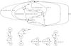	Fig. 1 Network graphs for H, He, C, Si, and O as the main hubs. Helium has been split into two small sub-networks, the one on the left showing the reactions with metals, and the one on the right the reactions with hydrogen-based species and photons. The network graphs can be obtained by using the KROME tool pathway.py.
Open with DEXTER

2.2. Chemical models

In this section we present different chemical models that can be employed in simulations of galaxy formation and evolution, together with the main physical ingredients that regulate the thermal evolution of the gas and its dynamics through the process of star formation. The models have been tested to work for a wide range of temperatures, namely from 10 to 10⁹ K. The single ingredients presented in this paper are all implemented in KROME and can be easily added and/or removed to create models of different complexity. Here we present models with increasing level of complexity as shown in Table 1.

Table 1

List of included thermal processes.

In the following we refer to the total number density (cm^-3) as n_tot, to the atomic neutral hydrogen (HI) number density as n_H, while the total density of hydrogen nuclei is denoted as (1)The number density of the single species j is given as n_j.

Table 2

List of photo-processes included in our chemical network.

2.2.1. Reaction rates

The first three models include a selection of the most important reactions to contribute to the formation or destruction of molecular hydrogen in a gas consisting of a mixture of H- and He-based species. It includes H, He, He⁺, He⁺⁺, H⁺, H⁻, H₂, H, and electrons. The aim of these models is to provide a minimal chemical network that is suitable for following the transition between the atomic and molecular gas phases, but keeps the computational cost at a reasonable level to be employed in 3D simulations of galaxy evolution. For users who are interested in a more detailed chemical model, a network including several metal species is outlined below and employed in Sect. 3.3. The list of reactions is reported in Table B.1, together with references, and is split into hydrogen/helium species and metals (C, C⁺, Si, Si⁺, Si⁺⁺, O, O⁺). We refer to the complete network as react_galaxy, downloadable with the KROME package². The rates for the metal network are adopted from Glover & Jappsen (2007) and are the same as employed in Bovino et al. (2014a). Three-body reactions are not included owing to the low-density regime involved in the physical problem considered here (with number densities up to 10⁴–10⁵ cm^-3).

In Fig. 1, we show a sketch of the complete chemical network, where we distinguish hydrogen, helium, and metal sub-networks with the most important paths to form and destroy the different species. As can be seen in Fig. 1, this is an H₂-oriented network that includes important reactions involving metals and helium. We have a total of 16 species and 74 reactions.

2.2.2. Photochemistry

The presence of a radiation background alters the chemical evolution by ionising and dissociating atoms and molecules. Here we consider the photo-processes reported in Table 2 due to a UVB/X-ray radiation background from quasars and galaxies (Haardt & Madau 2012) up to 100 keV. The cross-sections, where possible, have been taken from standard databases: the SWRI database³ and the Leiden database⁴. KROME also includes an internal database based on the work by Verner & Ferland (1996) and Verner et al. (1996). The frequency (energy) domain is divided by KROME into N bins and the photo-rates (k_ph), and the photo-heating rates (Γ_ph) are computed by employing the following discrete formulae,

where h is the Planck constant, J_i the radiation background in units of eV cm^-2 sr^-1 Hz^-1 s^-1, and σ_i and E₀ are, respectively, the cross-section (in cm²) and the threshold energy (in eV) of the given photo-process. Here, ⟨ E_i ⟩ = (E^R + E^L) / 2 is the average photon energy of a single bin of size ΔE = E^R − E^L, with R and L standing for RIGHT and LEFT. The final photo-rate is in units of s^-1.

The photo-heating rate (in eV s^-1) is then used to compute the final heating for every jth photo-process, with n_j being the abundance of the ionised or dissociated species in cm^-3.

In this work we used 10 000 photo-bins to ensure convergence on the final photo-rates⁵. These must be re-computed if the radiation background evolves over time. We considered an optically thin gas and a time-independent radiation background at redshift z = 3. A comparison of this background with other standard radiation fields is discussed in Sect. 3.2.1. The effect of reducing the incident radiation and adding shielding is also reported in the same section. We do not discuss here the photochemistry induced by galactic UV photons because this is strongly connected to the way the radiation is treated in hydrodynamical codes. For instance, the UV radiation should partly come from stellar sources within the galaxy and requires proper modelling of the radiative transfer. For more details on how to handle UV sources within simulations of galaxy evolution, we refer to previous work (Gnedin et al. 2009; Gnedin & Kravtsov 2011; Christensen et al. 2012; Tomassetti et al. 2015). However, KROME can handle any kind of radiation, so our discussion on how to compute the photo-rates does not change.

We note that KROME has been designed to be coupled with multi-frequency radiative transfer codes, and it provides a flexible interface that allows setting any bin-based discretization of the impinging radiation flux.

Table 3

List of included thermal processes.

2.2.3. Photodissociation of H₂

In the presence of an ionising radiation background, there are two processes that can photodissociate molecular hydrogen: (i) excitation to the vibrational continuum of an excited electronic state (P8 in Table 2); and (ii) the two-step Solomon process (P9 in Table 2). These processes have been proposed and widely discussed in Stecher & Williams (1967), Allison & Dalgarno (1969), Abel et al. (1997), Glover & Brand (2001), and Gay et al. (2012), and we refer to those papers for additional details. The two processes have different thresholds: the “direct” dissociation occurs for energies above 14.16 eV for ortho-hydrogen and 14.68 eV for para-hydrogen, and it is important in the presence of a strong ionising UV flux (e.g. in HII regions). The Solomon process occurs in the Lyman (B) and Werner (C) bands in a very tiny energy window (11.25–13.51 eV). For the “direct” process, we employ the fit proposed by Abel et al. (1997) based on the data by Allison & Dalgarno (1969), whereas the two-step Solomon process we employ the rate suggested by Glover & Jappsen (2007), given by (4)

2.3. Thermal processes

The thermal state of the gas is regulated by many processes, which we report in Table 3 and discuss in the following sections. Resolution limits in hydrodynamical simulations sometimes make it necessary to impose a temperature floor, which might also depend on the density. We apply it to the total cooling Λ(T) in the following way, (5)as for example in Safranek-Shrader et al. (2014). Even though the range of temperatures over which our modelling of thermal processes is valid is quite wide (10−10⁹ K, see Table 1), in most of the tests discussed in this work we assume a density-independent T_floor = 100 K, since most 3D hydrodynamical simulations of galaxy evolution, out of resolution concerns, cannot properly model colder gas. We remind the reader, however, that T_floor can be changed by the user, according to the problem and resources one has.

2.3.1. Atomic and molecular cooling

The standard atomic cooling (atom recombinations, collisional ionisations, excitations, and Bremsstrahlung of ions) and the Compton cooling from the cosmic microwave background (CMB) have been adopted from Cen (1992). H₂ roto-vibrational cooling is an update to Glover & Abel (2008), which includes the new rates reported by Glover (2015).

Following Hollenbach & McKee (1979) and Omukai (2000), we include chemical cooling coming from the destruction of H₂ in the gas phase (reactions 18, 19, in Table B.1). This is discussed in detail in the KROME paper (Grassi et al. 2014).

Recombination reactions on dust can also contribute to the cooling (see e.g. reactions 29, 30 in Table B.1). We have included this effect following Bakes & Tielens (1994), as discussed in Sect. 2.3.6.

2.3.2. Metal cooling in previous work

Cooling from metal line transitions is one of the most important contributions at low densities that regulates the thermal evolution of the gas and then the star formation process. The complexity of the interstellar medium (ISM) makes it challenging to evaluate it at run time even when we consider a sub-ensemble of the most important species (C, N, O, Ne, Si, Mg, S, Ca, and Fe). The large amount of ionisation states, transitions, and collisional processes (and different colliders) makes in fact the problem computationally prohibitive within hydrodynamical simulations, as we should solve a linear system of equations within every chemical time step to calculate the level populations for every metal species and then the cooling efficiencies. This problem has been extensively discussed in the literature, and there has been a lot of effort to produce simplified models or to provide cooling tables that can be easily employed in hydrodynamic simulations.

Cooling tables for metals have been calculated over the years in different ways and assuming different approximations, and they turned out to be the most common approach in simulations of galaxies and of the intergalactic medium. We can distinguish between four different cases: pure collisional ionisation equilibrium (CIE) tables (Sutherland & Dopita 1993), collisional ionisation non-equilibrium (CINe) tables (Gnat & Sternberg 2007; Gnat & Ferland 2012), tables that consider a photoionising background in photoionisation equilibrium (PIE) as in Wiersma et al. (2009), and photoionisation non-equilibrium (PINe) tables, such as the recent tables reported by Vasiliev (2011) and Oppenheimer & Schaye (2013). Richings et al. (2014) extended these tables to a wider range of densities and improved the model below 10⁴ K for C and O.

Most of these tables were calculated with the photoionisation code CLOUDY (Ferland et al. 1998). Usually CLOUDY provides equilibrium cooling tables (CIE or PIE), which are evaluated at a fixed temperature, density, and metallicity (Z/Z_⊙), evolving the system to reach the equilibrium (when ionisations balance recombinations). In the approach by Gnat & Sternberg (2007), Vasiliev (2011), and Oppenheimer & Schaye (2013), who explored the effect of non-equilibrium chemistry on the final cooling functions, CLOUDY was mainly used to evaluate the cooling functions, by requiring the non-equilibrium ionisation fractions of the metal ions species evaluated as input by solving a system of ODEs over the time, for a given temperature and density.

Gnat & Sternberg (2007) computed the cooling without any ionisation background, i.e. in collisional ionisation non-equilibrium, and provided tables for the non-equilibrium ion fractions x_ion and ion-by-ion cooling efficiencies Λ_e,ion. The sum of ionic cooling efficiencies, weighted by the non-equilibrium ion densities, then provides an efficient way to compute the total cooling of a given metal. They report clear examples on how to use the cooling tables in Gnat & Ferland (2012). The final total cooling rate is written as Λ_tot = n_e ∑ _j(n_j ∑ _ionx_j,ionΛ_e,ion), with n_j being the total amount of the considered coolant metal, and the ion subscript runs over the ionisation states of the jth metal.

Vasiliev (2011) provides cooling tables for the gas exposed to different radiation backgrounds evaluating the non-equilibrium ionisation fractions by adopting a similar approach to the one in Gnat & Sternberg (2007). They explored low density gas and different metallicites going from 10^-3 to 1 Z_⊙ and showed that assuming PIE leads to an overestimate of the cooling for T>10⁶ K, since the gas in non-equilibrium stays overionised. At higher densities, collisions dominate photoionisations and this effect is reduced. An increase in the radiation strength decreases the final cooling rate further.

The recent work by Oppenheimer & Schaye (2013) provides an additional overview on the effect of the radiation and non-equilibrium chemistry on the metal cooling efficiencies. Their approach works better for T> 10⁴ K because they assume that the collisions are dominated by electrons, but if radiation is included they can consider the results below T< 10⁴ K as reasonable. They explored the four approaches discussed above, namely the CIE, CINe, PIE, and PINe, and compared the results, focussing mostly on the regime of temperatures above 10⁴ K. An important final statement of their work is that the presence of a radiation background suppresses cooling either in equilibrium or non-equilibrium.

2.3.3. Metal cooling in KROME

For the metal cooling at T ≥ 10⁴ K we employ an updated version of the PIE tables presented by Shen et al. (2010), which have been computed with CLOUDY 10.1 in the presence of the extragalactic radiation by Haardt & Madau (2012). The tables are valid in a range of temperatures between 10 ≤ T ≤ 10⁹ K, density 10^-9 ≤ n_{H_tot} ≤ 10⁴ cm^-3, and redshift 0 ≤ z ≤ 15.1, and they scale linearly with the metallicity: (6)The equilibrium cooling computed by Shen et al. (2010) includes all metals up to an atomic number of 30 (Zn). The H and He contributions are not included since they are computed time-dependently based on the non-equilibrium chemical evolution. The heating rate coming from the photoionisation of metals is also included in the same fashion. In Fig. 2 we show the equilibrium metal cooling function for densities of 10^-5 cm^-3 and 1 cm^-3 and at redshift z = 3, for the cases with and without radiation at a metallicity Z = 0.5 Z_⊙. Those cooling functions are comparable to the former work by Shen et al. (2010), where they also included the contribution coming from H and He that we do not show here.

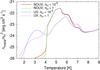	Fig. 2 Metal line cooling from equilibrium (PIE) tables for a gas of metallicity Z = 0.5 Z_⊙ at redshift z = 3. The case without a radiation background (NOUV) and with a radiation background (UV) are both shown for two different densities: n = 10^-5 and n = 1 cm^-3.
Open with DEXTER

KROME includes the machinery to solve the linear system for the individual metal excitation levels time-dependently for temperatures below 10⁴ K, and it provides the non-equilibrium metal cooling for the most important atoms and ions⁶. This method has been tested in a recent study by Bovino et al. (2014a), and includes the non-equilibrium cooling of C, C⁺, Si, Si⁺, O, O⁺, Fe, and Fe⁺, as described in Grassi et al. (2014) based on Glover & Jappsen (2007), and Maio et al. (2007). Richings et al. (2014) have shown that in the presence of a strong photoionising background like the one employed in this work, the most important coolants at T< 10⁴ K are C⁺, Si⁺, and Fe⁺, together with hydrogen. In general at low temperatures or higher densities, the excess of electrons favours forbidden line transitions of low-ionised metals such as C, C⁺, Si, Si⁺, and O, as also reported by Shen et al. (2010) and Wolfire et al. (2003). Our non-equilibrium approach below 10⁴ K is able to capture the most important metal contributions to the total cooling function in an accurate way, i.e. solving the non-equilibrium system at run time according to the network we employ in our simulations.

It is worth noting that this approach is different from the non-equilibrium tables computed for example by Vasiliev (2011) and Oppenheimer & Schaye (2013) (PINe approach), which depend not only on the initial conditions (i.e. ionic composition and temperature) employed to solve the system of ODEs (Vasiliev et al. 2010), but are also bound to a fixed chemical network that in most cases does not include molecules. Our cooling is instead accurately evaluated on the fly according to the evolution of the given chemical network (that can change), and is fully consistent with the conditions explored in the physical problem users want to pursue.

The final metal cooling in the temperature range of 10–10⁹ K is then expressed as a combination of equilibrium and non-equilibrium cooling, (7)where f₁ and f₂ are two functions that allow a smooth transition between equilibrium and non-equilibrium cooling around T = 10⁴ K and are defined as with c_sm = 10^-3 and f₁(T) + f₂(T) = 1, for every T. The smoothing factor c_sm is needed to help the solver reach the convergence.

Given the temperature range of validity for the equilibrium table, one can choose between a simple approach (Eq. (6)) over the whole range or a more sophisticated treatment (Eq. (7)). The aim of this work is in fact to release a chemical model within the publicly available package KROME, which can be easily modified by the users to allow a lower or higher degree of complexity in large scale simulations.

2.3.4. Dust cooling

The dust cooling is calculated based on Hollenbach & McKee (1979), who employ the following expression, (10)where n_tot and n_d are the total gas number density and the grain number density, respectively; πa² is the dust grain effective cross-section, with a being the grain size; v_g is the gas velocity defined as , with m_p being the proton mass; and T_d is the dust temperature. In the following, we assume for simplicity a constant dust temperature of 10 K, which is typical of molecular clouds. The user is, however, free to adopt a different description, for instance calculating the dust temperature from the heating-cooling balance of the grains (Grassi et al. 2014). When the dust is hotter than the gas (i.e. T_d>T), Eq. (10) acts as a heating term for the gas.

We tabulate the dust cooling similarly to the H₂ formation rate on dust as explained in Sect. 2.4, and we show in Sect. 3.1 that, under the conditions discussed here, its effect is negligible.

2.3.5. H₂ photo-heating

The most important contribution to the heating of the gas under the conditions discussed in this paper is the photo-heating. We include the photo-heating of atoms and molecules due to ionisations and photodissociations. The latter also include the H₂ UV pumping and H₂ direct photodissociation heating as explained below.

The energy budget produced by the Solomon process is converted into heating through two different paths: the direct dissociation, which provides 0.4 eV as kinetic energy, and the energy released by collisional de-excitation of the excited vibrational levels of the H₂ electronic ground state, which is commonly called H₂ UV pumping heating. The final heating is the sum of the two contributions and is given by (11)where

The total heating Γ_tot(H₂) is expressed in terms of erg cm^-3 s^-1. We have followed Burton et al. (1990), Glover & Jappsen (2007), and Draine & Bertoldi (1996), who assume that the pumping rate is 8.5 times higher than the photodissociation rate k_ph(H₂). The critical density n_cr is the density at which the collisional de-excitations become comparable to the spontaneous radiative processes, i.e. this process only becomes important for n_{H_tot} ≥ n_cr, which is ~10⁴ cm^-3. For the definition of the n_cr, we refer to Hollenbach & McKee (1979; see also Omukai 2000).

2.3.6. Photoelectric heating by dust grains

UV radiation with photon energies of about 6 eV or more can remove electrons from interstellar dust grains (GR), which increase the energy of the surrounding gas by subsequent Coulomb collisions. This heating process is called dust photoelectric effect and is due to the reactions (14)where q ≥ 0 is the charge number. The above process is often in competition with its inverse, the recombination reaction (15)which removes energy from the gas producing cooling. The net dust photoelectric heating has been parametrized by Bakes & Tielens (1994), who introduced the charging parameter(16)with G₀ being the Habing flux and n_e the electron number density in cm^-3 . We obtain G₀ by summing the flux over the photo-bins, which are in the range between 6–13.6 eV, normalized to the average interstellar radiation field flux 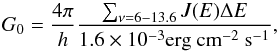(17)as reported by Omukai et al. (2008).

The net photoelectric heating is defined as with the efficiency (21)

2.3.7. Chemical heating

Chemical heating from exothermic reactions that form H₂ both in the gas phase and on dust is included following Grassi et al. (2014), Hollenbach & McKee (1979), and Omukai (2000).

2.4. H₂ formation on dust

The H₂ formation on dust is particularly relevant because it determines the atomic-to-molecular transition in the gas phase, which is one of the most efficient formation paths for H₂. In previous work (Gnedin et al. 2009; Gnedin & Kravtsov 2011; Christensen et al. 2012), a constant rate originally obtained by Jura (1975) was employed, with the addition of a clumping factor (C_ρ) intended to address the subgrid nature of H₂ formation in unresolved high-density regions, namely (22)The constant 3 × 10^-17 has been motivated by observational measurements. We note that other versions of this rate have been proposed that include an explicit temperature dependency via a sticking coefficient (Tomassetti et al. 2015).

KROME allows the user to employ different types of dust with a given Mathis, Rumpl, & Nordsieck (MRN)–like distribution ~a^{− α} (Mathis et al. 1977) and to customize the range of sizes that can also extend to the regime of the polycyclic aromatic hydrocarbons (PAHs). We note here that there are different ways to treat the PAHs (Li & Draine 2001; Tielens 2010) and that the PAH distribution is usually different from a standard power law (Weingartner & Draine 2001a).

KROME employs the H₂ formation on dust based on Cazaux & Spaans (2009). They provide the rates for carbon and silicon-based grains as (23)where each ith bin of the two grain species (i.e. C and Si) contributes to the total amount of molecular hydrogen formation. In the above equation n_H is the number density of atomic hydrogen in the gas-phase, v_g is the gas thermal velocity, n_ij the number density of the jth dust type in the ith bin, a_ij its size. Here, T and are the temperatures of the gas and of the dust in the ith bin, respectively. The function ϵ_j has two expressions depending on the type of grain considered and has been reported by Cazaux & Spaans (2009). The sticking coefficient is given as (24)with T₂ ≡ T/ (100 K), according to Hollenbach & McKee (1979). We note that a clumping factor can also be applied to this rate.

Since we are not interested in following the dust evolution (i.e. sputtering, growth, and shuttering processes are neglected), we can tabulate the H₂ formation on dust improving the performances of the code without losing accuracy. The final rates are provided as tables using the following expression (25)with μ being the mean molecular weight. The details of the dust tabulation will be discussed in a forthcoming paper (Grassi et al., in prep.), where we will show a series of 3D hydrodynamic applications.

For this work we have prepared tables at a constant dust temperature T_d = 10 K following the results discussed by Richings et al. (2014), but a time-dependent T_d table can also be provided on request. We show in Appendix A that the on-the-fly approach, in which T_d is evaluated by solving the thermal balance equation (see Grassi et al. 2014), produces identical results to the case when T_d is kept constant. At the low densities considered in this work, T_d is not strongly affected by the interaction between dust and gas.

2.5. Adiabatic index and mean molecular weight

When coupling chemistry with hydrodynamics, different caveats arise. Two of the prevailing problems are the correct treatment of the adiabatic index (γ) and the mean molecular weight (μ). Both quantities strongly depend on the chemical composition of the gas and are used to convert, for instance, pressure to energy to temperature through the ideal gas equation of state,

where m_H is the hydrogen mass, and e the specific energy per unit mass.

KROME is able to evaluate the adiabatic index in different ways, allowing a strong flexibility to the users. A simple temperature-independent approach has been presented in Grassi et al. (2014), and a more detailed method employs the calculation of the roto-vibrational partition functions, which provides a temperature-dependent adiabatic index⁷. Because we work in a low-density regime and want to keep the approach simple, here we have decided to employ a constant adiabatic index, namely γ = 5 / 3, which is typical of a monoatomic or a collisionless gas.

We use the μ computed by KROME based on the species abundances to have a fully consistent model. Our final mean molecular weight is the summation of different contributions: where x_j are the species mass fractions, Z is the metallicity in mass fraction, and we have assumed a mean mass number (number of protons+neutrons) for metals ⟨ A ⟩ _metals = 17.6003. If other He-based or H-based species are added to the chemical network, the above definitions of the individual mean molecular weight should be updated. This is usually done automatically by KROME during the pre-processing stage.

3. Testing the models

In the following we show how the different ingredients of our model affect the chemical and thermal evolution of the gas. We distinguish between two classes of models (see Table 1): (i) Models I and II without any radiation background; and (ii) Models III and IV, which include the radiation background of Haardt & Madau (2012) and can be employed to study the chemical evolution in galaxy simulations and follow the HII-HI-H₂ phase transitions. In the following tests, we used a simple one-zone cloud collapse model (Omukai 2000), which evolves the density ρ based on the free-fall time t_ff, (33)with , where G is the gravitational constant. The thermal evolution was solved with Eq. (33) as (34)We have already shown (Grassi et al. 2014) that KROME is able to reproduce previous results obtained by employing the above one-zone framework (Omukai 2000), so we consider this problem a reliable test for exploring the physics discussed in this work. The choice of performing one-zone cloud collapse tests is also due to the possibility of dynamically exploring the chemical and thermal evolution at different densities, to resemble the transition through the different gas phases. In Sect. 3.3 we additionally present tests at fixed densities, i.e. a time evolution of an isochoric gas.

3.1. The neutral models

Models I and II in Table 1 are based on low-complexity networks, and they include approximate metal cooling, i.e. a network composed of a mixture of H/He-based species, with the equilibrium metal tables discussed in Sect. 2.3. The two models employ different H₂ formation rates on dust: (i) Model I employs the approximated H₂ formation rate on dust (Eq. (22)), which does not depend on the dust composition or the dust size distribution and is widely used in galaxy simulations; and (ii) Model II employs an improved dust treatment including dust tables evaluated as discussed in Sect. 2.4. These tables assume 40 bins in size of dust grains of mixed composition including carbonaceous (20 bins) and silicates (20 bins) with a fixed dust temperature T_d = 10 K. The metallicity is kept constant as Z = 0.5 Z_⊙, and we show how the metallicity affects the results in Sect. 3.2.1. We evolve the one-zone collapse starting with the following initial conditions: T = 100 K, n_tot = 1 cm^-3, n_H = 0.92 n_tot, n_He = 0.0755 n_tot, n_H⁺ = n_e = 10^-4n_tot, n_H₂ = 10^-6n_tot, which we evolve until a density of 10⁶ cm^-3 is reached. The other species abundances are set to zero. For Model II we use a standard MRN dust distribution (a^-3.5), which scales as D = D_⊙ × Z/Z_⊙, where D_⊙ = 0.00934 is the dust-to-gas mass ratio at solar metallicity. In addition to this we evolve the same Model II, but including dust cooling (referred to as Model IIa) to assess the impact of this contribution on the thermal evolution.

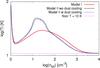Fig. 3

Thermal evolution versus the total number density for the three models described in Sect. 3.1. The red curve refers to Model I, which employs a simple prescription for the H₂ formation rate on dust. The black curve employs the more accurate Cazaux & Spaans (2009) rate for H₂ formation on dust, and the blue curve is the same Model II, but including the dust cooling as reported in Eq. (10). The magenta line represents the CMB floor at z = 3.

Open with DEXTER

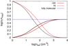	Fig. 4 H₂ and H number fraction as a function of the total number density. Red curves refer to Model I, and black curves to Model II. Model II with dust cooling is not reported here because it overlaps the case without dust cooling.
Open with DEXTER

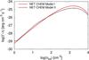	Fig. 5 H₂ net chemical heating as a function of the total number density. The red curve represents Model I, and the black curve refers to Model II.
Open with DEXTER

In Fig. 3 we report the thermal evolution of the gas as a function of the total number density for the three models presented above. The H₂ formation on dust computed with a proper dust model produces a hotter gas around 10¹–10² cm^-3. This is mainly because more heating is produced from the formation of H₂ caused by an increase in the formation efficiency due to the rate by Cazaux & Spaans (2009). The increase is also clear from Fig. 4, where the evolution of atomic and molecular hydrogen (in terms of n_i/n_{H_tot}) is shown for the two models. In Fig. 5 we report the net H₂ formation heating | Γ − Λ |. In the case where a proper dust model is included, the transition HI-H₂ occurs a bit earlier. The effect of dust cooling (Model IIa) at these densities is in practice negligible (Fig. 3).

3.2. Models irradiated by UVB/X-ray photons

We now explore what happens to a gas of metallicity Z = 0.5 Z_⊙ under a UVB/X-ray radiation background computed at redshift z = 3. In the first of these models (Model III in Table 1) we include the H/He photo-processes reported in Table 2 and photo-heating, together with a proper treatment of the photoelectric heating by dust. This model is compared to Model I discussed in the previous section, which includes the approximate H₂ formation rate on dust. Here we have added the photochemistry for consistency and refer to it as Model Ia. An additional parameter in Model Ia is the clumping factor C_ρ, for which we explore the results of C_ρ = 1 and C_ρ = 10, the latter enhancing the H₂ formation on dust by an order of magnitude. We assume here a gas at T = 2 × 10⁴ K, with a slightly lower density compared to Models I and II (i.e. n_tot = 0.1 cm^-3), and a fully ionised chemical composition. The results are reported in Fig. 6.

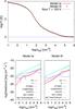	Fig. 6 Top: thermal evolution as a function of the total number density for Model Ia (with a clumping factor C_ρ = 1) and Model III. Bottom: heating and cooling functions versus the total number density for Model Ia (left) and Model III (right). We omit here the model with clumping factor C_ρ =10, since this is identical to Model Ia.
Open with DEXTER

Two important pieces of information can be retrieved from this test: (i) Under the conditions considered in this simple test, having an approximate H₂ formation rate on dust or a more accurate treatment does not affect the thermal evolution; (ii) changing the clumping factor in Model Ia, i.e. increasing the H₂ formation rate on dust by an order of magnitude also has a negligible effect on the final thermal evolution. For this reason we only report in Fig. 6 a comparison between Model Ia (C_ρ = 1) and Model III. This behaviour can be better understood if we look at the different heating/cooling contributions for the evolution of the gas irradiated by a UVB/X-ray background (bottom panels of Fig. 6). The thermal evolution in both models is dominated by photo-heating and metal line cooling, which balance each other out, while the net chemical heating has no influence at all on the final evolution. This is the effect of the ionising background, which also produces a warmer gas. As a result, the effect of having a different H₂ formation rate on dust is negligible for the thermal evolution. The atomic cooling controls the evolution along with the photoelectric heating by dust.

When we look at the HII-HI-H₂ transition (Fig. 7), however, to change the H₂ formation rate on dust produces a difference. For instance, employing an accurate and appropriate grain size-dependent approach (Model III) leads to the transition at lower densities compared to the approximated rate (black curves in the plot). The gas becomes fully molecular (n_H₂/n_{H_tot} = 0.5) earlier. If we increase the clumping factor by an order of magnitude, then the density at which the gas becomes fully molecular is also reduced by an order of magnitude. This holds for both the approximate rate (Model Ia) and the rate provided by Cazaux & Spaans (2009). We conclude that it is very important to include a proper dust treatment (grain size-dependent) to accurately assess the atomic-to-molecular transition in galaxy evolution simulations. We also note that the clumping factor is making a large difference. It is quite common in hydrodynamic simulations of galaxy evolution to set this parameter to C_ρ=10 or even higher values (Gnedin et al. 2009), inducing a faster HI-H₂ transition to account for unresolved high-density gas. If the need for such a clumping factor, however, also prevails in higher resolution simulations, it may also point towards an underestimate of the H₂ formation rates. At the same time, we note that the HII-HI transition is completely dominated by photo-chemistry and results in an identical evolution for the three models discussed in this section.

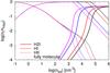	Fig. 7 H₂ and H number fraction as a function of the total number density. Black curves refer to Model Ia, red curves to Model III, blue curves to Model Ia but with a clumping factor C_ρ = 10, and magenta curves to Model III but with the H₂ formation rate 10 times higher.
Open with DEXTER

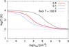	Fig. 8 Thermal evolution for Model III at three different metallicities, namely Z = 0.1 Z_⊙, 0.5 Z_⊙, and Z_⊙ (solar metallicity). The temperature floor is sketched by the magenta line.
Open with DEXTER

3.2.1. Effects of the radiation background and metallicity

As already reported by Richings et al. (2014), the type of radiation background, its strength, and the metallicity can affect the evolution of the gas (and, subsequently, the star formation) as they change the ionisation processes and the dust and metal related physics.

Here we present three models with different metallicities, namely Z/Z_⊙ = 0.1, 0.5, and 1 (i.e. solar metallicity). The metallicity affects both the metal cooling and the H₂ formation on dust, which have a linear dependence on it. In Fig. 8 we see the boosting of metal cooling when going from lower to higher metallicities. The effect of metallicity on H₂ formation reported in Fig. 9 plays a relevant role, since it is more evident when we switch from 0.1 Z_⊙ to solar metallicity with a difference of two orders of magnitude in the density level at which the fully molecular stage is reached. Changing the metallicity then has the same effect as enhancing the rate of H₂ formation on dust.

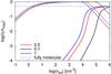	Fig. 9 Atomic and molecular hydrogen evolution for three different metallicities, Z = 0.1 Z_⊙, 0.5 Z_⊙, and Z_⊙ (solar metallicity), for Model III. The fully molecular stage is indicated by the horizontal dotted line.
Open with DEXTER

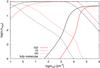	Fig. 10 Ionised, atomic, and molecular hydrogen evolution as a function of the density for two different radiation backgrounds, the standard extragalactic background at redshift z = 3 (red curves) by Haardt & Madau (2012), and 10 per cent of the latter (black curves). The results come from the evolution of Model III.
Open with DEXTER

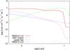	Fig. 11 Different radiation backgrounds as a function of energy up to 13.6 eV. Red solid curve and magenta curve: extragalactic radiation background from Haardt & Madau (2012) at redshift z = 3 and z = 0, respectively; green dotted curve: the standard ISRF by Draine (1978); blue dashed curve: a simple power-law spectrum. See text for details.
Open with DEXTER

Since we are employing a very strong photoionising radiation background, it is important to assess the differences produced once we change this radiation background. Taking ten per cent of the extragalactic radiation background produces a significant effect in the HII-HI-H₂ transitions because fewer ionisations occur, and the atomic phase is reached much earlier, thereby boosting the formation of H₂ at lower densities (Fig. 10). This can be considered as mimicking the effect of the shielding produced by a radiative transfer algorithm, which indeed will tend to strongly reduce the ionisation processes in dense regions.

We note here that the radiation background at redshift z = 3 is quite strong and comparable to the galactic radiation produced by stellar sources. We report in Fig. 11 a comparison of different radiation backgrounds for energies up to 13.6 eV: the extragalactic radiation by Haardt & Madau (2012) at z = 3 and z = 0 (commonly employed in galaxy simulations), the interstellar radiation field (ISRF) by Draine (1978), and a typical power-law radiation background (E/E₀)^-1, with E₀ = 13.6 eV. The ISRF by Draine (1978) is comparable to the extragalactic radiation background by Haardt & Madau (2012), which is even stronger at lower energies.

3.3. The effect of non-equilibrium metal cooling

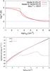Fig. 12

Top: thermal evolution for Model III (red) and Model IV (black) as a function of the total number density. Bottom: main cooling/heating functions for the two models. Red curves refer to Model III and black curves to Model IV. The different contributions reported in the figure are the following: atomic cooling (dotted lines), metal cooling (dashed lines), and photo-heating (solid lines).

Open with DEXTER

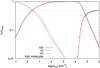Fig. 13

Chemical evolution of H₂, H⁺, and H as a function of the total number density for Model III, which employs the equilibrium metal cooling at all temperatures (red curves), and Model IV, which employs the non-equlibrium metal cooling for temperature T< 10⁴ K (black curves and crosses). The effect of non-equilibrium cooling on the H₂ evolution is negligible and produces the same results as the equilibrium cooling model (crosses). A horizontal line at n_i/n_{H_tot} = 0.5 is sketched to represent the fully molecular stage.

Open with DEXTER

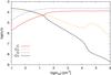	Fig. 14 Most relevant metal species number fraction evolution (C, C⁺, O, and O⁺) as a function of the total number density.
Open with DEXTER

As already discussed in Sect. 2.3, non-equilibrium metal line cooling, i.e. solving the linear system at run time for the excitation levels of every single metal, can have an impact on the evolution of the gas at temperatures T< 10⁴ K. In Model IV, we evolve the H/He mixture network plus seven additional metal species (C, C⁺, O, O⁺, Si, Si⁺, and Si⁺⁺) and reactions involving these metals as listed in Table B.1. In the end we have a network with 16 species and 74 reactions that we evolve with conditions similar to the one employed in the previous tests, i.e. a fully ionised gas at T = 2 × 10⁴ K. The metal number densities are initialised by rescaling the solar abundances by the metallicity Z/Z_⊙. The main difference between Model III (discussed in the previous section) and the current Model IV is the treatment of the metal cooling below 10⁴ K, where we employ Eq. (7) for the non-equilibrium treatment.

In the top panel of Fig. 12 we show the comparison between Models III and IV, to see how much the thermal evolution is affected by the different treatment of metal line cooling. When we employ the non-equilibrium approach we have less net cooling. If we look at the bottom panel of Fig. 12, we see a difference in the two metal cooling functions of about ten per cent, which increases at higher densities (n_tot = 1−10² cm^-3), and then the two contributions equate each other as the collisions dominate the photoionisations, as already discussed in Sect. 2.3.

In Figs. 13 and 14, we report the evolution of the hydrogen and metal species as a function of density, respectively. When we employ the non-equilibrium cooling, the evolution of the hydrogen species (and in particular the HI-H₂ transition) is not affected at all, since the cooling only changes the thermal evolution at low densities. We argue that there is only a minor effect mainly in the HII-HI transition. However, it could be important to assess how much the dynamics and the structure of the galaxy are affected in a realistic 3D simulation. Figure 14 shows how quickly the most relevant metal ions recombine. This occurs at high densities when the temperature is lowered and recombinations become faster.

For a self-consistent comparison between a non-equilibrium and a photoionisation equilibrium approach, we prepared a test that evolves (below 10⁴ K) the full system of ODEs for a long enough time to reach the thermo-chemical equilibrium by employing our non-equilibrium metal cooling; i.e. the system is evaluated on the fly. In this way we can provide important information about the time scale to reach equilibrium and understand when an equilibrium approach is correct and when it is leading to an overestimate or underestimate of the cooling. For reference we took a typical integration time step for galaxy simulations, which can be estimated to be ~10⁴ yr, even if we consider that a large change in the thermochemical conditions may reduce the hydrodynamical time step in order to take their effect into account. We evolved the system for two different constant densities (isochoric evolution) and four different initial temperatures and show the results in Fig. 15. Since this is a thermochemical equilibrium, the system will reach the same final equilibrium temperature T_eq for the same gas density.

The equilibrium is reached at different times, and this obviously depends on the density: a higher density gas reaches the equilibrium much earlier. If we consider a typical numerical time step of 10⁴ yr, it is clear that assuming equilibrium for low-density gas leads to a large error in the cooling because the equilibrium needs at least 1 Myr to be reached. However, in situations where the density is high, the time for the system to reach equilibrium is comparable to 10⁴ yr, and then this assumption becomes valid on small scales.

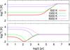	Fig. 15 Gas thermal evolution for two different densities, 0.1 cm^-3 (top panel) and 100 cm^-3 (bottom panel), and starting from four different temperatures: 500, 1000, 5000, and 9000 K. The system is evolved until it reaches the thermo-chemical equilibrium.
Open with DEXTER

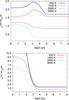	Fig. 16 Time evolution of the non-equilibrium/equilibrium metal cooling ratio for two different densities, 0.1 cm^-3 (top panel) and 100 cm^-3 (bottom panel), for four different temperatures as reported in the legend.
Open with DEXTER

As a second test, we evolved the system with a CLOUDY-like approach, i.e. not only keeping the density constant but also the temperature and evolving the system until it reaches the chemical equilibrium. The aim of this test was to quantify the differences between the non-equilibrium and the equilibrium cooling and, in particular, how far our approach is from the standard CLOUDY equilibrium tables (PIE). In Fig. 16 we show the ratio Λ^non−eq/ Λ^eq for two different constant densities, 0.1 cm^-3 (top panel) and 100 cm^-3 (bottom panel), and for four different initial temperatures: 500, 1000, 5000, and 9000 K. It is worth noting that there are cases where assuming the equilibrium might lead to a large overestimate or underestimate of the final metal cooling. From this simple test we can infer that (i) the non-equilibrium cooling for temperatures below 5000 K is larger than the equilibrium cooling by a factor of two and for high densities by orders of magnitude. This can be because our approach includes collisions with neutral species like H and H₂, while the CLOUDY tables assume the collisions to be dominated by electrons. (ii) When we compare the equilibrium reached with our approach versus CLOUDY, i.e. at the plateau (for times greater than 1 Myr or less depending on the density and temperature), we see that the differences are about a factor of two. This behaviour may be due to the different number of metals, transitions, and colliders between our approach and the CLOUDY one. We also note that the chemical network is different. In most cases, the time to reach equilibrium is longer than a typical hydrodynamical time step for temperatures below 1000 K, so a non-equilibrium approach is then desirable. Our results also agree with recent similar tests reported by Richings et al. (2014), who have shown that non-equilibrium cooling is usually enhanced compared to the equilibrium case. It is important to note that we are not comparing the net cooling here because we are only interested in the differences between the metal cooling. Obviously the photo-heating in the non-equilibrium and equilibrium cases will be different, as well as other cooling/heating contributions that can change the final real effect on the thermal evolution of the gas, as for instance in the test reported in Sect. 3.3, which provided less net cooling in the non-equilibrium case.

3.4. Radiation attenuation and caveats

In the tests presented in the previous sections, we focussed on the optically thin case and employed only the extragalactic radiation background by Haardt & Madau (2012). For a realistic study of galaxy properties, it is necessary to include a proper radiative transfer module that follows the history of photons during the simulation. A local UV radiation background produced by the stars is also a desirable ingredient and can be much stronger than the extragalactic background (see discussion in Sect. 3.2.1). This piece of information should therefore come from a more accurate radiative transfer treatment. The computational cost of coupling radiative transfer with chemistry is not negligible, and over the years local approximations have been proposed.

Since this problem does not concern the model presented here and pursued with the package KROME, we next only show some simple tests to illustrate some of the results. For this purpose, we assumed that the UV flux provided to KROME had already been obtained from a radiative transfer calculation, so that the UV radiation could be treated in the optically thin approximation. For the photodissociation of H₂, self-shielding and shielding by dust may be relevant, however, and we explore here how much it matters within the one-zone framework.

An optical depth is commonly applied to the optically thin rates assuming τ = ∑ _iσ_iN_i, with σ_i being the photo cross-section of the ith species and N_i the column density, which is evaluated in different ways and in general depends on a characteristic length, (35)where L_i is often based on a velocity or density gradient (i.e. a Sobolev-like length) or on the Jeans length, as in the tests reported in this work.

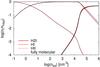	Fig. 17 Chemical evolution of H₂, H⁺, and H as a function of the total number density n_tot, for Model III with and without self-shielding as discussed in Sect. 3.4. A line at n_i/n_{H_tot} = 0.5 is sketched to represent the fully molecular stage.
Open with DEXTER

We focus on H₂ and dust shielding, which provide an optically thick rate of (36)where S_self is adopted by Wolcott-Green et al. (2011), and S_d is defined following Richings et al. (2014) as (37)with γ_H₂ = 3.74, N_{H_tot} = N_HI + N_HII + 2N_H₂, and σ_d = 4.0 × 10^-22 cm². We note here that Gnedin et al. (2009) and Gnedin & Kravtsov (2011) use different values for σ_d. We assume here a column density based on the Jeans length λ_J, which is suitable for the one-zone collapse problem: 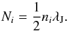(38)As we show in Fig. 17, the shielding is not relevant for our test case. This is mainly because in the presence of a fixed ionising background, photo-heating is very strong and the high temperature delays the formation of molecular hydrogen, since collisional dissociation is an efficient destruction channel above 2000 K.

It is important to note here that the above formulation of the self-shielding comes from a static slab of gas and that the Jeans length generally overestimates the column density (Wolcott-Green et al. 2011). To properly evaluate the column density and then the H₂ shielding, we would need to probe the relative velocity between particles and compare it with the thermal velocity. This can be assessed with algorithms such as TREECOL (Clark et al. 2012; Hartwig et al. 2015). However, this is again an issue of modelling radiation transfer that does not concern the microphysics and the chemistry solved by KROME. Seifried & Walch (2015) have recently reported 3D calculations of collapsing ISM filaments where the TREECOL algorithm has been successfully coupled with KROME and we refer interested readers to this paper.

Moreover, as pointed out by Richings et al. (2014), to apply an optical depth to the optically thin atomic photo-rates within the chemical solver is computationally unfeasible, and it is rather inaccurate because it does not consider the geometry, the photon history, and the environment. It is then crucial to have a radiation attenuation coming from the solution of the radiative transfer equation. In addition, some colleagues pursue simpler approaches, like the one presented by Christensen et al. (2012) and Tomassetti et al. (2015), which provide reasonable results for the average atomic-to-molecular transition in galaxy simulations, while of course local variations exist and are expected within real galaxies.

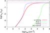	Fig. 18 Chemical evolution for H₂ as a function of the total number density for different physical conditions, C_ρ = 10, Z = Z_⊙, and z = 0 without shielding (red curve), and with shielding (blue curve), and our reference model with C_ρ = 1, Z = 0.5 Z_⊙, z = 3, labelled as Model Ia (green curve).
Open with DEXTER

To provide a more reasonable test and to show the effect of the shielding on H₂, we perform runs that resemble the conditions often employed in galaxy simulations: solar metallicity, an extragalactic background corresponding to a redshift z = 0, and a clumping factor of at least C_ρ = 10, all parameters that boost the formation of H₂, allowing its formation at densities where the shielding becomes important (n_tot ~ 10 cm^-3). In these tests we keep the approach simple and consistent with previous models, employing the H₂ formation rate on dust used in Gnedin et al. (2009), Gnedin & Kravtsov (2011), Christensen et al. (2012), and discussed in our Sect. 2.4. In Fig. 18 we report the results with and without H₂ shielding, together with our reference case where we do not have any shielding, and assume C_ρ = 1, Z = 0.5 Z_⊙, and z = 3 (Model Ia). An increase in metallicity and a decrease in redshift boost the formation of H₂ as already discussed in Sect. 3.2.1, together with a high clumping factor. Compared to our reference model (Model Ia), the transition to a fully molecular phase is reached around 10³ cm^-3, which shifts to 10² cm^-3 once we also include the shielding. This agrees with previous 3D results (Gnedin et al. 2009), which showed a fully molecular stage between 10²–10³ cm^-3 depending on the parameters employed (e.g. radiation strengths, dust-to-gas ratio, clumping factor, etc.). This test suggests that once we employ a weaker background, it mimics the effect of radiation attenuation, and the shielding has an impact on the final results, in this specific case shifting the HI-H₂ transition to lower densities by a factor of an order of magnitude.

To summarize, the results obtained by the suite of tests we performed for this work, based on the models reported in Table 1, suggest that

The HI-H₂ transition strongly depends on the metallicity, the radiation background strength, and the clumping factor, three parameters that affect the H₂ formation rate on dust. However, in high-resolution studies, where the clumping factor is not needed, it is very important to employ an accurate treatment of the dust grains. We showed that employing a formation rate that depends on the grain size is more efficient in forming H₂.
The non-equilibrium metal cooling is very important at low density (n_tot< 10 cm^-3), and it is in general higher than what the equilibrium tables provide. We showed that this also depends on the physical conditions, i.e. density and temperature.
The shielding is important, but it should be coupled with a proper radiative transfer module, which can produce a reasonably attenuated radiation background taking the geometry and the photon history into account.

Overall, the models presented and tested in this work are appropriate for studying the different gas phase transitions in galaxy simulations and can follow the evolution of key observational tracers, such as CII. This is the first chemical model for the ISM of galaxies publicly released through the package KROME, and it can be employed in different hydrodynamical codes (e.g. ENZO, FLASH, RAMSES, and GASOLINE), providing a high degree of flexibility. We discuss in the next section some additional physical processes that could be added to the basic models we presented in the previous sections.

3.5. Additional ingredients and final remarks

To have a comprehensive chemical model for galaxies, additional ingredients can be considered besides the ones discussed in the previous sections. Cosmic rays and X-ray primary and secondary ionisations can be included in the chemical network presented here together with the resulting Coulomb heating. While it has been shown by Richings et al. (2014) that secondary ionisation is not relevant, cosmic-ray ionisation becomes important in shielded regions as is typical of molecular clouds. A list of important ionisation and dissociation reactions involving cosmic rays is reported in Table B.2 as taken from KIDA (Wakelam et al. 2012). The heating released into the gas by each of these reactions is assumed to be 20 eV. We note that there are detailed calculations on the heating released by cosmic-ray ionisation, and a density dependent function has been provided, for example, in Glassgold et al. (2012). The X-ray physics, in contrast, is beyond the scope of this work, but as it is already part of the package KROME, the users can incorporate it into the current framework if relevant.

Both for comparison with observational data and for a higher complexity, the current network can be extended to include CO, as in the network by Glover et al. (2010) released with KROME. However, we note that the aim of this work is to provide chemical models that can be easily (and without too much computational demand) embedded in hydrodynamical simulations, so we decided to present low-complexity models that are nevertheless able to capture the most important physics needed to follow the HII-HI-H₂ transition. In addition, it was shown by Glover & Clark (2012) that the SFR might be insensitive to the molecular content and that having H₂ or CO cooling is not a necessary condition to form stars. They showed that other processes, like the fine-structure emission by C⁺ at low densities and the gas-grain energy transfer at high densities, are in fact very efficient coolants and that the shielding of the ISRF by dust is the main parameter affecting the star formation process.

The models reported in this work not only include state-of-the-art chemistry and microphysics, but should be considered as an update to previous models (e.g. Krumholz et al. 2008; Gnedin et al. 2009; Gnedin & Kravtsov 2011) and also an extension and improvement, in particular, for the accuracy of the different ingredients employed in KROME. The present framework is released with KROME and it is publicly accessible. It represents one of the few attempts to share a common chemistry module that can be employed to assess a quantitative comparison between different hydrodynamical codes. We note that the AGORA project (Kim et al. 2014), which aims to provide a robust code comparison of galaxy simulations, is mainly oriented to the study of the atomic phase, while here we present models that can be used for different gas phase transitions and most importantly can be extended and customized by the users.

4. Conclusions

In this paper we have presented different chemical models (networks and microphysics), which can be employed in 3D simulations of galaxy formation and evolution, as well as in similar environments. We cover in fact a density range from 10^-8 to 10⁴ cm^-3 and a wide temperature range of 10–10⁹ K. The upper limit in densities is mainly dictated by the limit in the equilibrium cooling tables by Shen et al. (2010). Our chemical network has been carefully checked to be valid in the whole range of temperatures. We included the most important cooling functions, heating processes, dust physics, and photochemical processes suitable for this kind of studies. These models have been presented within the framework of the astrochemistry package KROME. An interface to some of the most used hydrodynamic codes has already been released with the package (FLASH, ENZO, and RAMSES), but these models can be employed in any hydrodynamical code through an interface to KROME, as we will show in a forthcoming paper where we use the smoothed-particle-hydrodynamic code GASOLINE to explore the gas phase transitions in an isolated galaxy simulation. The aim of the paper is to provide a flexible model where every single ingredient can be added or removed based on the applications and the computational demand of a given problem.

Different one-zone collapse tests have been presented to study the effect of the most important ingredients on the thermal evolution of the gas and on the transitions between different phases. In particular, we have explored different prescriptions for the H₂ formation on dust with focus on an accurate treatment of the dust physics. Employing a proper dust grain distribution and the accurate rate by Cazaux & Spaans (2009) boosts the formation of H₂, shifting the atomic-to-molecular transition to lower densities. However, we also noticed that in the presence of a strong ionising radiation background, the gas remains ionised up to densities of 10 cm^-3, and the efficient photo-heating delays the formation of H₂. To elucidate this point we performed a series of tests where we varied the clumping factor (which boosts the H₂ formation rate on dust) and decreased the radiation background by a factor of 10. In both cases we found that the transition shifts to lower densities, an effect that is stronger in the case of a lower radiation background. It is then necessary to include a proper radiation attenuation in 3D simulations. We also tested the effect of introducing a simple recipe for the H₂ shielding, but since the thermal evolution is driven here by the photoionisation of hydrogen (and the consequent photo-heating), the effect of H₂ self-shielding turned out to be negligible. A radiative transfer algorithm is then more appropriate for accurately studying the transitions between the different gas phases.

In the end, the main parameters discussed in this work need to be carefully checked based on the physical application and possibly on observational data. For instance, a combination of C_ρ = 10, a higher rate for H₂ formation on dust, low-radiation background (e.g. at z = 0), and shielding leads to reasonable gas phase transitions, but this cannot be considered as the only applicable case.

We also discussed the effect of employing the non-equilibrium metal cooling below 10⁴ K versus an equilibrium treatment. This is in general computationally more expensive, since we need to solve a linear system of equations “on the fly” and add more species and reactions to our network, because we need to follow the non-equilibrium abundances of the various metals coolants. It turned out that by using the photoionisation equilibrium tables from CLOUDY below 10⁴ K can lead to inaccurate results if, depending on the density, the system is far from equilibrium.

We show that the non-equilibrium metal cooling is in general higher than the photoionised equilibrium metal tables, and our equilibrium produces results that differ by about a factor of 2 compared to CLOUDY. We attribute these differences to the different metals, transitions, and chemical networks employed. A non-equilibrium approach is in any case preferable for temperatures below 10⁴ K, as also discussed, under different conditions and approaches, in previous papers (Vasiliev 2011; Oppenheimer & Schaye 2013; Richings et al. 2014). The metal network is likewise important if we want to assess a comparison between theory and observations, for instance on the 158 μm CII emission band.

The chemical network and the KROME options files are publicly available at http://bitbucket/tgrassi/krome and ready to be used with the codes that are already interfaced with the package, but also via a custom interface to other framework codes. In addition, we can provide dust tables on request for different conditions when needed.

¹

www.kromepackage.org

²

https://bitbucket.org/tgrassi/krome

³

http://phidrates.space.swri.edu

⁴

http://home.strw.leidenuniv.nl/~ewine/photo/

⁵

This is an input parameter for KROME that can be easily customized by the users, as well as the bins’ spacing and their energy position.

⁶

The approach to evaluating the metal line cooling has general validity but, due to the limited validity range of the collisional rates, we can only apply it below 10⁴ K.

⁷

See https://bitbucket.org/tgrassi/krome/wiki

Acknowledgments

We are very grateful to Sijing Shen for having provided the CLOUDY metal cooling tables and for fruitful discussions on this topic. S.B., D.R.G.S. and R.B. thank the DFG for funding via the Schwerpunktprogram SPP 1573 “Physics of the Interstellar Medium” under grants # BO 4113/1-2, SCHL 1964/1-2, and BA 3706/3-2. T.G. acknowledges the Centre for Star and Planet Formation funded by the Danish National Research Foundation. P.R.C. acknowledges research funding by the Deutsche Forschungsgemeinschaft (DFG) Sonderforschungsbereiche (SFB) 963 and support by the Tomalla Foundation. We thank the referee for the useful comments.

References

Abel, T., Anninos, P., Zhang, Y., & Norman, M. L. 1997, New Astron., 2, 181 [NASA ADS] [CrossRef] [Google Scholar]
Aldrovandi, S. M. V., & Pequignot, D. 1973, A&A, 25, 137 [NASA ADS] [Google Scholar]
Allison, A. C., & Dalgarno, A. 1969, Atomic Data, 1, 91 [NASA ADS] [CrossRef] [Google Scholar]
Bañados, E., Decarli, R., Walter, F., et al. 2015, ApJ, 805, L8 [NASA ADS] [CrossRef] [Google Scholar]
Bakes, E. L. O., & Tielens, A. G. G. M. 1994, ApJ, 427, 822 [NASA ADS] [CrossRef] [Google Scholar]
Barlow, S. E. 1984, Ph.D. Thesis, University of Colorado at Boulder [Google Scholar]
Bigiel, F., Leroy, A., Walter, F., et al. 2008, AJ, 136, 2846 [NASA ADS] [CrossRef] [Google Scholar]
Bigiel, F., Leroy, A., Walter, F., et al. 2010, AJ, 140, 1194 [NASA ADS] [CrossRef] [Google Scholar]
Bovino, S., Grassi, T., Schleicher, D. R. G., & Latif, M. A. 2014a, ApJ, 790, L35 [NASA ADS] [CrossRef] [Google Scholar]
Bovino, S., Latif, M. A., Grassi, T., & Schleicher, D. R. G. 2014b, MNRAS, 441, 2181 [NASA ADS] [CrossRef] [Google Scholar]
Braun, H., & Schmidt, W. 2012, MNRAS, 421, 1838 [NASA ADS] [CrossRef] [Google Scholar]
Burton, M. G., Hollenbach, D. J., & Tielens, A. G. G. M. 1990, ApJ, 365, 620 [NASA ADS] [CrossRef] [Google Scholar]
Capitelli, M., Coppola, C. M., Diomede, P., & Longo, S. 2007, A&A, 470, 811 [NASA ADS] [CrossRef] [EDP Sciences] [Google Scholar]
Carilli, C. L., & Walter, F. 2013, ARA&A, 51, 105 [NASA ADS] [CrossRef] [Google Scholar]
Cazaux, S., & Spaans, M. 2009, A&A, 496, 365 [NASA ADS] [CrossRef] [EDP Sciences] [Google Scholar]
Cen, R. 1992, ApJS, 78, 341 [NASA ADS] [CrossRef] [Google Scholar]
Christensen, C., Quinn, T., Governato, F., et al. 2012, MNRAS, 425, 3058 [NASA ADS] [CrossRef] [Google Scholar]
Clark, P. C., Glover, S. C. O., & Klessen, R. S. 2012, MNRAS, 420, 745 [NASA ADS] [CrossRef] [Google Scholar]
Coppola, C. M., Longo, S., Capitelli, M., Palla, F., & Galli, D. 2011, ApJS, 193, 7 [NASA ADS] [CrossRef] [Google Scholar]
Corrigan, S. J. B. 1965, J. Chem. Phys., 43, 4381 [NASA ADS] [CrossRef] [Google Scholar]
Dalgarno, A., & Lepp, S. 1987, in Astrochemistry, eds. M. S. Vardya, & S. P. Tarafdar, IAU Symp., 120, 109 [Google Scholar]
de Jong, T. 1972, A&A, 20, 263 [NASA ADS] [Google Scholar]
Dove, J. E., Rusk, A. C. M., Cribb, P. H., & Martin, P. G. 1987, ApJ, 318, 379 [NASA ADS] [CrossRef] [Google Scholar]
Draine, B. T. 1978, ApJS, 36, 595 [NASA ADS] [CrossRef] [Google Scholar]
Draine, B. T., & Bertoldi, F. 1996, ApJ, 468, 269 [NASA ADS] [CrossRef] [Google Scholar]
Federrath, C. 2013, MNRAS, 436, 3167 [NASA ADS] [CrossRef] [Google Scholar]
Federrath, C., Schrön, M., Banerjee, R., & Klessen, R. S. 2014, ApJ, 790, 128 [NASA ADS] [CrossRef] [Google Scholar]
Ferland, G. J., Peterson, B. M., Horne, K., Welsh, W. F., & Nahar, S. N. 1992, ApJ, 387, 95 [NASA ADS] [CrossRef] [Google Scholar]
Ferland, G. J., Korista, K. T., Verner, D. A., et al. 1998, PASP, 110, 761 [NASA ADS] [CrossRef] [Google Scholar]
Gay, C. D., Abel, N. P., Porter, R. L., et al. 2012, ApJ, 746, 78 [NASA ADS] [CrossRef] [Google Scholar]
Glassgold, A. E., Galli, D., & Padovani, M. 2012, ApJ, 756, 157 [NASA ADS] [CrossRef] [Google Scholar]
Glover, S. C. O. 2015, MNRAS, 451, 2082 [NASA ADS] [CrossRef] [Google Scholar]
Glover, S. C. O., & Abel, T. 2008, MNRAS, 388, 1627 [NASA ADS] [CrossRef] [Google Scholar]
Glover, S. C. O., & Brand, P. W. J. L. 2001, MNRAS, 321, 385 [NASA ADS] [CrossRef] [Google Scholar]
Glover, S. C. O., & Clark, P. C. 2012, MNRAS, 421, 9 [NASA ADS] [Google Scholar]
Glover, S. C. O., & Jappsen, A.-K. 2007, ApJ, 666, 1 [NASA ADS] [CrossRef] [Google Scholar]
Glover, S. C. O., Federrath, C., Mac Low, M.-M., & Klessen, R. S. 2010, MNRAS, 404, 2 [NASA ADS] [Google Scholar]
Gnat, O., & Ferland, G. J. 2012, ApJS, 199, 20 [NASA ADS] [CrossRef] [Google Scholar]
Gnat, O., & Sternberg, A. 2007, ApJS, 168, 213 [NASA ADS] [CrossRef] [Google Scholar]
Gnedin, N. Y., & Kravtsov, A. V. 2011, ApJ, 728, 88 [NASA ADS] [CrossRef] [Google Scholar]
Gnedin, N. Y., Tassis, K., & Kravtsov, A. V. 2009, ApJ, 697, 55 [NASA ADS] [CrossRef] [Google Scholar]
Grassi, T., Krstic, P., Merlin, E., et al. 2011, A&A, 533, A123 [NASA ADS] [CrossRef] [EDP Sciences] [Google Scholar]
Grassi, T., Bovino, S., Schleicher, D. R. G., et al. 2014, MNRAS, 439, 2386 [NASA ADS] [CrossRef] [MathSciNet] [Google Scholar]
Grete, P., Vlaykov, D. G., Schmidt, W., Schleicher, D. R. G., & Federrath, C. 2015, New J. Phys., 17, 023070 [NASA ADS] [CrossRef] [Google Scholar]
Haardt, F., & Madau, P. 2012, ApJ, 746, 125 [NASA ADS] [CrossRef] [Google Scholar]
Hartwig, T., Glover, S. C. O., Klessen, R. S., Latif, M. A., & Volonteri, M. 2015, MNRAS, 452, 1233 [NASA ADS] [CrossRef] [Google Scholar]
Hindmarsh, A. C. 1983, IMACS Transactions on Scientific Computation, 1, 55 [Google Scholar]
Hollenbach, D., & McKee, C. F. 1979, ApJS, 41, 555 [NASA ADS] [CrossRef] [Google Scholar]
Hopkins, P. F., Kereš, D., Oñorbe, J., et al. 2014, MNRAS, 445, 581 [NASA ADS] [CrossRef] [Google Scholar]
Hu, C.-Y., Naab, T., Walch, S., Glover, S. C. O., & Clark, P. C. 2015, MNRAS, 458, 3528 [NASA ADS] [CrossRef] [Google Scholar]
Janev, R. K., Langer, W. D., & Evans, K. 1987, Elementary processes in Hydrogen-Helium plasmas – Cross sections and reaction rate coefficients [Google Scholar]
Jura, M. 1975, ApJ, 197, 575 [NASA ADS] [CrossRef] [Google Scholar]
Karpas, Z., Anicich, V., & Huntress, W. T. 1979, J. Chem. Phys., 70, 2877 [NASA ADS] [CrossRef] [Google Scholar]
Katz, H., Sijacki, D., & Haehnelt, M. G. 2015, MNRAS, 451, 2352 [NASA ADS] [CrossRef] [Google Scholar]
Kennicutt, Jr., R. C. 1989, ApJ, 344, 685 [NASA ADS] [CrossRef] [Google Scholar]
Kennicutt, Jr., R. C. 1998, ApJ, 498, 541 [NASA ADS] [CrossRef] [Google Scholar]
Kim, J.-h., Abel, T., Agertz, O., et al. 2014, ApJS, 210, 14 [NASA ADS] [CrossRef] [Google Scholar]
Kimura, M., Lane, N. F., Dalgarno, A., & Dixson, R. G. 1993, ApJ, 405, 801 [NASA ADS] [CrossRef] [Google Scholar]
Kingdon, J. B., & Ferland, G. J. 1996, ApJS, 106, 205 [NASA ADS] [CrossRef] [Google Scholar]
Kreckel, H., Bruhns, H., Čížek, M., et al. 2010, Science, 329, 69 [NASA ADS] [CrossRef] [Google Scholar]
Krumholz, M. R. 2012, ApJ, 759, 9 [NASA ADS] [CrossRef] [Google Scholar]
Krumholz, M. R., McKee, C. F., & Tumlinson, J. 2008, ApJ, 689, 865 [NASA ADS] [CrossRef] [Google Scholar]
Krumholz, M. R., Dekel, A., & McKee, C. F. 2012, ApJ, 745, 69 [NASA ADS] [CrossRef] [Google Scholar]
Kuhlen, M., Krumholz, M. R., Madau, P., Smith, B. D., & Wise, J. 2012, ApJ, 749, 36 [NASA ADS] [CrossRef] [Google Scholar]
Latif, M. A., Bovino, S., Van Borm, C., et al. 2014, MNRAS, 443, 1979 [NASA ADS] [CrossRef] [Google Scholar]
Latif, M. A., Bovino, S., Grassi, T., Schleicher, D. R. G., & Spaans, M. 2015a, MNRAS, 446, 3163 [NASA ADS] [CrossRef] [Google Scholar]
Latif, M. A., Omukai, K., Habouzit, M., Schleicher, D. R. G., & Volonteri, M. 2015b, MNRAS, submitted [arXiv:1509.07034] [Google Scholar]
Le Teuff, Y. H., Millar, T. J., & Markwick, A. J. 2000, A&AS, 146, 157 [NASA ADS] [CrossRef] [EDP Sciences] [MathSciNet] [PubMed] [Google Scholar]
Lenzuni, P., Chernoff, D. F., & Salpeter, E. E. 1991, ApJS, 76, 759 [NASA ADS] [CrossRef] [Google Scholar]
Leroy, A. K., Walter, F., Brinks, E., et al. 2008, AJ, 136, 2782 [NASA ADS] [CrossRef] [Google Scholar]
Li, A., & Draine, B. T. 2001, ApJ, 554, 778 [NASA ADS] [CrossRef] [Google Scholar]
Maio, U., Dolag, K., Ciardi, B., & Tornatore, L. 2007, MNRAS, 379, 963 [NASA ADS] [CrossRef] [Google Scholar]
Maiolino, R., Carniani, S., Fontana, A., et al. 2015, MNRAS, 452, 54 [NASA ADS] [CrossRef] [Google Scholar]
Mathis, J. S., Rumpl, W., & Nordsieck, K. H. 1977, ApJ, 217, 425 [NASA ADS] [CrossRef] [Google Scholar]
McKee, C. F., & Ostriker, J. P. 1977, ApJ, 218, 148 [NASA ADS] [CrossRef] [Google Scholar]
Mitchell, G. F., & Deveau, T. J. 1983, ApJ, 266, 646 [NASA ADS] [CrossRef] [Google Scholar]
Nahar, S. N. 1995, ApJS, 101, 423 [NASA ADS] [CrossRef] [Google Scholar]
Nahar, S. N. 1996, ApJS, 106, 213 [NASA ADS] [CrossRef] [Google Scholar]
Nahar, S. N. 1999, ApJS, 120, 131 [NASA ADS] [CrossRef] [MathSciNet] [Google Scholar]
Nahar, S. N. 2000, ApJS, 126, 537 [NASA ADS] [CrossRef] [Google Scholar]
Nahar, S. N., & Pradhan, A. K. 1997, ApJS, 111, 339 [NASA ADS] [CrossRef] [Google Scholar]
Offner, S. S. R., Klein, R. I., McKee, C. F., & Krumholz, M. R. 2009, ApJ, 703, 131 [NASA ADS] [CrossRef] [Google Scholar]
Omukai, K. 2000, ApJ, 534, 809 [NASA ADS] [CrossRef] [Google Scholar]
Omukai, K., Schneider, R., & Haiman, Z. 2008, ApJ, 686, 801 [NASA ADS] [CrossRef] [Google Scholar]
Oppenheimer, B. D., & Schaye, J. 2013, MNRAS, 434, 1043 [NASA ADS] [CrossRef] [Google Scholar]
Pelupessy, F. I., & Papadopoulos, P. P. 2009, ApJ, 707, 954 [NASA ADS] [CrossRef] [Google Scholar]
Pineda, J. L., Langer, W. D., & Goldsmith, P. F. 2014, A&A, 570, A121 [NASA ADS] [CrossRef] [EDP Sciences] [Google Scholar]
Poulaert, G., Brouillard, F., Claeys, W., McGowan, J. W., & Van Wassenhove, G. 1978, J. Phys. B, 11, L671 [NASA ADS] [CrossRef] [Google Scholar]
Prieto, J., Jimenez, R., Haiman, Z., & González, R. E. 2015, MNRAS, 452, 784 [NASA ADS] [CrossRef] [Google Scholar]
Richings, A. J., & Schaye, J. 2016, MNRAS, 458, 270 [NASA ADS] [CrossRef] [Google Scholar]
Richings, A. J., Schaye, J., & Oppenheimer, B. D. 2014, MNRAS, 440, 3349 [NASA ADS] [CrossRef] [Google Scholar]
Safranek-Shrader, C., Milosavljević, M., & Bromm, V. 2014, MNRAS, 438, 1669 [NASA ADS] [CrossRef] [Google Scholar]
Salim, D. M., Federrath, C., & Kewley, L. J. 2015, ApJ, 806, L36 [NASA ADS] [CrossRef] [Google Scholar]
Savin, D. W., Krstić, P. S., Haiman, Z., & Stancil, P. C. 2004, ApJ, 606, L167 [NASA ADS] [CrossRef] [Google Scholar]
Schleicher, D. R. G., Bovino, S., Latif, M. A., Ferrara, A., & Grassi, T. 2016, A&A, 585, A11 [NASA ADS] [CrossRef] [EDP Sciences] [Google Scholar]
Schmidt, M. 1959, ApJ, 129, 243 [NASA ADS] [CrossRef] [Google Scholar]
Schmidt, M. 1963, ApJ, 137, 758 [NASA ADS] [CrossRef] [Google Scholar]
Schmidt, W., & Federrath, C. 2011, A&A, 528, A106 [NASA ADS] [CrossRef] [EDP Sciences] [Google Scholar]
Schneider, I. F., Dulieu, O., Giusti-Suzor, A., & Roueff, E. 1994, ApJ, 424, 983 [NASA ADS] [CrossRef] [Google Scholar]
Schruba, A., Leroy, A. K., Walter, F., et al. 2011, AJ, 142, 37 [NASA ADS] [CrossRef] [Google Scholar]
Seifried, D., & Walch, S. 2015, MNRAS, submitted [arXiv:1510.06544] [Google Scholar]
Semenov, V. A., Kravtsov, A. V., & Gnedin, N. Y. 2015, ArXiv e-prints [arXiv:1512.03101] [Google Scholar]
Shapiro, P. R., & Kang, H. 1987, ApJ, 318, 32 [NASA ADS] [CrossRef] [Google Scholar]
Shen, S., Wadsley, J., & Stinson, G. 2010, MNRAS, 407, 1581 [NASA ADS] [CrossRef] [Google Scholar]
Somerville, R. S., Popping, G., & Trager, S. C. 2015, MNRAS, 453, 4337 [NASA ADS] [CrossRef] [Google Scholar]
Stancil, P. C., Havener, C. C., Krstić, P. S., et al. 1998, ApJ, 502, 1006 [NASA ADS] [CrossRef] [Google Scholar]
Stancil, P. C., Schultz, D. R., Kimura, M., et al. 1999, A&AS, 140, 225 [NASA ADS] [CrossRef] [EDP Sciences] [Google Scholar]
Stecher, T. P., & Williams, D. A. 1967, ApJ, 149, L29 [NASA ADS] [CrossRef] [Google Scholar]
Stenrup, M., Larson, Å., & Elander, N. 2009, Phys. Rev. A, 79, 012713 [NASA ADS] [CrossRef] [Google Scholar]
Sutherland, R. S., & Dopita, M. A. 1993, ApJS, 88, 253 [NASA ADS] [CrossRef] [Google Scholar]
Tielens, A. G. G. M. 2010, The Physics and Chemistry of the Interstellar Medium (Cambridge University Press) [Google Scholar]
Tomassetti, M., Porciani, C., Romano-Díaz, E., & Ludlow, A. D. 2015, MNRAS, 446, 3330 [NASA ADS] [CrossRef] [Google Scholar]
Vasiliev, E. O. 2011, MNRAS, 414, 3145 [NASA ADS] [CrossRef] [Google Scholar]
Verner, D. A., & Ferland, G. J. 1996, ApJS, 103, 467 [NASA ADS] [CrossRef] [Google Scholar]
Verner, D. A., Ferland, G. J., Korista, K. T., & Yakovlev, D. G. 1996, ApJ, 465, 487 [NASA ADS] [CrossRef] [Google Scholar]
Vasiliev, E. O., Sethi, S. K., & Nath, B. B. 2010, ApJ, 719, 1343 [NASA ADS] [CrossRef] [Google Scholar]
Voronov, G. S. 1997, Atom. Data Nucl. Data Tables, 65, 1 [NASA ADS] [CrossRef] [Google Scholar]
Wakelam, V., Herbst, E., Loison, J.-C., et al. 2012, ApJS, 199, 21 [NASA ADS] [CrossRef] [Google Scholar]
Weingartner, J. C., & Draine, B. T. 2001a, ApJ, 548, 296 [NASA ADS] [CrossRef] [Google Scholar]
Weingartner, J. C., & Draine, B. T. 2001b, ApJ, 563, 842 [NASA ADS] [CrossRef] [Google Scholar]
Wiersma, R. P. C., Schaye, J., & Smith, B. D. 2009, MNRAS, 393, 99 [NASA ADS] [CrossRef] [Google Scholar]
Wolcott-Green, J., Haiman, Z., & Bryan, G. L. 2011, MNRAS, 418, 838 [NASA ADS] [CrossRef] [Google Scholar]
Wolfire, M. G., McKee, C. F., Hollenbach, D., & Tielens, A. G. G. M. 2003, ApJ, 587, 278 [NASA ADS] [CrossRef] [Google Scholar]
Wong, T., & Blitz, L. 2002, ApJ, 569, 157 [NASA ADS] [CrossRef] [Google Scholar]
Yoshida, N., Omukai, K., Hernquist, L., & Abel, T. 2006, ApJ, 652, 6 [NASA ADS] [CrossRef] [Google Scholar]
Zhao, L. B., Stancil, P. C., Gu, J. P., et al. 2004, ApJ, 615, 1063 [NASA ADS] [CrossRef] [Google Scholar]

Appendix A: Dust temperature evolution

In this section we relax the assumption made on the dust temperature and let it evolve over time. In this case we keep the same grain distribution, i.e. 40 bins of carbonaceous and astronomical silicates, with a typical power law (dn/da ∝ a^-3.5), and instead of employing the dust tables, we solve (by means of a root-finding procedure) the following thermal balance equation at run time: (A.1)The terms reported in the above equation depend on the grain size a, the radiation frequency ν, and gas and dust temperatures, T and T_d. For details on Eq. (A.1) and on how every single term is defined, see Grassi et al. (2014). In Fig. A.1 we report the thermal evolution of the gas, together with the dust temperature for the different types of dust taking the largest and the smallest in size. We also plot the results obtained keeping the dust temperature constant at 10 K (same as in Fig. 6). As one can see from the figure, the dust temperature for all the grains is almost constant. It increases slightly only for the largest grains at high density, but the differences are not appreciable. The thermal evolution of the gas in the two cases is exactly the same. This confirms that the

assumption to keep the dust temperature constant over the range of densities explored here is valid.

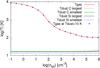	Fig. A.1 Thermal evolution for Model III and the dust temperature for the largest and smallest dust grains. Both silicates (Si) and carbonaceous (C) grains are reported. The dust temperature is obtained solving the thermal balance between the emitted and absorbed radiation and gas-grain thermal exchange (see Eq. (A.1) in the text).
Open with DEXTER

Appendix B: Reaction rates employed in the present work

In the following tables we list the reaction rates employed in the present work. These are publicly available with the KROME package under the folder KROME/NETWORKS, named react_galaxy.

Table B.1

List of reactions and rates included in our chemical network.

continued.

continued.

continued.

Cosmic rays related reactions.

Table B.3

Fit coefficients for the charge transfer reaction .

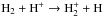All Tables

Table 1

List of included thermal processes.

In the text

Table 2

List of photo-processes included in our chemical network.

In the text

Table 3

List of included thermal processes.

In the text

Table B.1

List of reactions and rates included in our chemical network.

continued.

continued.

continued.

Cosmic rays related reactions.

In the text

Table B.3

Fit coefficients for the charge transfer reaction .

In the text

All Figures

	Fig. 1 Network graphs for H, He, C, Si, and O as the main hubs. Helium has been split into two small sub-networks, the one on the left showing the reactions with metals, and the one on the right the reactions with hydrogen-based species and photons. The network graphs can be obtained by using the KROME tool pathway.py.
Open with DEXTER
In the text

	Fig. 2 Metal line cooling from equilibrium (PIE) tables for a gas of metallicity Z = 0.5 Z_⊙ at redshift z = 3. The case without a radiation background (NOUV) and with a radiation background (UV) are both shown for two different densities: n = 10^-5 and n = 1 cm^-3.
Open with DEXTER
In the text

	Fig. 3 Thermal evolution versus the total number density for the three models described in Sect. 3.1. The red curve refers to Model I, which employs a simple prescription for the H₂ formation rate on dust. The black curve employs the more accurate Cazaux & Spaans (2009) rate for H₂ formation on dust, and the blue curve is the same Model II, but including the dust cooling as reported in Eq. (10). The magenta line represents the CMB floor at z = 3.
Open with DEXTER
In the text

	Fig. 4 H₂ and H number fraction as a function of the total number density. Red curves refer to Model I, and black curves to Model II. Model II with dust cooling is not reported here because it overlaps the case without dust cooling.
Open with DEXTER
In the text

	Fig. 5 H₂ net chemical heating as a function of the total number density. The red curve represents Model I, and the black curve refers to Model II.
Open with DEXTER
In the text

	Fig. 6 Top: thermal evolution as a function of the total number density for Model Ia (with a clumping factor C_ρ = 1) and Model III. Bottom: heating and cooling functions versus the total number density for Model Ia (left) and Model III (right). We omit here the model with clumping factor C_ρ =10, since this is identical to Model Ia.
Open with DEXTER
In the text

	Fig. 7 H₂ and H number fraction as a function of the total number density. Black curves refer to Model Ia, red curves to Model III, blue curves to Model Ia but with a clumping factor C_ρ = 10, and magenta curves to Model III but with the H₂ formation rate 10 times higher.
Open with DEXTER
In the text

	Fig. 8 Thermal evolution for Model III at three different metallicities, namely Z = 0.1 Z_⊙, 0.5 Z_⊙, and Z_⊙ (solar metallicity). The temperature floor is sketched by the magenta line.
Open with DEXTER
In the text

	Fig. 9 Atomic and molecular hydrogen evolution for three different metallicities, Z = 0.1 Z_⊙, 0.5 Z_⊙, and Z_⊙ (solar metallicity), for Model III. The fully molecular stage is indicated by the horizontal dotted line.
Open with DEXTER
In the text

	Fig. 10 Ionised, atomic, and molecular hydrogen evolution as a function of the density for two different radiation backgrounds, the standard extragalactic background at redshift z = 3 (red curves) by Haardt & Madau (2012), and 10 per cent of the latter (black curves). The results come from the evolution of Model III.
Open with DEXTER
In the text

	Fig. 11 Different radiation backgrounds as a function of energy up to 13.6 eV. Red solid curve and magenta curve: extragalactic radiation background from Haardt & Madau (2012) at redshift z = 3 and z = 0, respectively; green dotted curve: the standard ISRF by Draine (1978); blue dashed curve: a simple power-law spectrum. See text for details.
Open with DEXTER
In the text

	Fig. 12 Top: thermal evolution for Model III (red) and Model IV (black) as a function of the total number density. Bottom: main cooling/heating functions for the two models. Red curves refer to Model III and black curves to Model IV. The different contributions reported in the figure are the following: atomic cooling (dotted lines), metal cooling (dashed lines), and photo-heating (solid lines).
Open with DEXTER
In the text

	Fig. 13 Chemical evolution of H₂, H⁺, and H as a function of the total number density for Model III, which employs the equilibrium metal cooling at all temperatures (red curves), and Model IV, which employs the non-equlibrium metal cooling for temperature T< 10⁴ K (black curves and crosses). The effect of non-equilibrium cooling on the H₂ evolution is negligible and produces the same results as the equilibrium cooling model (crosses). A horizontal line at n_i/n_{H_tot} = 0.5 is sketched to represent the fully molecular stage.
Open with DEXTER
In the text

	Fig. 14 Most relevant metal species number fraction evolution (C, C⁺, O, and O⁺) as a function of the total number density.
Open with DEXTER
In the text

	Fig. 15 Gas thermal evolution for two different densities, 0.1 cm^-3 (top panel) and 100 cm^-3 (bottom panel), and starting from four different temperatures: 500, 1000, 5000, and 9000 K. The system is evolved until it reaches the thermo-chemical equilibrium.
Open with DEXTER
In the text

	Fig. 16 Time evolution of the non-equilibrium/equilibrium metal cooling ratio for two different densities, 0.1 cm^-3 (top panel) and 100 cm^-3 (bottom panel), for four different temperatures as reported in the legend.
Open with DEXTER
In the text

	Fig. 17 Chemical evolution of H₂, H⁺, and H as a function of the total number density n_tot, for Model III with and without self-shielding as discussed in Sect. 3.4. A line at n_i/n_{H_tot} = 0.5 is sketched to represent the fully molecular stage.
Open with DEXTER
In the text

	Fig. 18 Chemical evolution for H₂ as a function of the total number density for different physical conditions, C_ρ = 10, Z = Z_⊙, and z = 0 without shielding (red curve), and with shielding (blue curve), and our reference model with C_ρ = 1, Z = 0.5 Z_⊙, z = 3, labelled as Model Ia (green curve).
Open with DEXTER
In the text

	Fig. A.1 Thermal evolution for Model III and the dust temperature for the largest and smallest dust grains. Both silicates (Si) and carbonaceous (C) grains are reported. The dust temperature is obtained solving the thermal balance between the emitted and absorbed radiation and gas-grain thermal exchange (see Eq. (A.1) in the text).
Open with DEXTER
In the text

Current usage metrics show cumulative count of Article Views (full-text article views including HTML views, PDF and ePub downloads, according to the available data) and Abstracts Views on Vision4Press platform.

Data correspond to usage on the plateform after 2015. The current usage metrics is available 48-96 hours after online publication and is updated daily on week days.

Initial download of the metrics may take a while.

A chemical model for the interstellar medium in galaxies

1. Introduction

2. Microphysics

2.1. The KROME package

2.2. Chemical models

2.2.1. Reaction rates

2.2.2. Photochemistry

2.2.3. Photodissociation of H2

2.3. Thermal processes

2.3.1. Atomic and molecular cooling

2.3.2. Metal cooling in previous work

2.3.3. Metal cooling in KROME

2.3.4. Dust cooling

2.3.5. H2 photo-heating

2.3.6. Photoelectric heating by dust grains

2.3.7. Chemical heating

2.4. H2 formation on dust

2.5. Adiabatic index and mean molecular weight

3. Testing the models

3.1. The neutral models

3.2. Models irradiated by UVB/X-ray photons

3.2.1. Effects of the radiation background and metallicity

3.3. The effect of non-equilibrium metal cooling

3.4. Radiation attenuation and caveats

3.5. Additional ingredients and final remarks

4. Conclusions

Acknowledgments

References

Appendix A: Dust temperature evolution

Appendix B: Reaction rates employed in the present work

All Tables

All Figures

2.2.3. Photodissociation of H₂

2.3.5. H₂ photo-heating

2.4. H₂ formation on dust