| Issue |
A&A
Volume 590, June 2016
|
|
|---|---|---|
| Article Number | A70 | |
| Number of page(s) | 7 | |
| Section | Interstellar and circumstellar matter | |
| DOI | https://doi.org/10.1051/0004-6361/201528012 | |
| Published online | 12 May 2016 | |
Feature-tailored spectroscopic analysis of the supernova remnant Puppis A in X-rays
1
Instituto de Astronomía y Física del Espacio (IAFE),
CC 67 – Suc. 28 (C1428ZAA),
CABA,
Argentina
e-mail:
This email address is being protected from spambots. You need JavaScript enabled to view it.
2
XMM-Newton Science Operations Centre, ESAC, Villafranca del
Castillo, 28080
Madrid,
Spain
3
Telespazio Vega UK LTD, Luton, Bedfordshire, LU1 3LU, UK
4
FADU, University of Buenos Aires, 1428
Buenos Aires,
Argentina
Received: 19 December 2015
Accepted: 23 March 2016
Abstract
We introduce a distinct method for performing spatially resolved spectral analysis of astronomical sources with highly structured X-ray emission. The method measures the surface brightness of neighboring pixels to adaptively size and shape each region, thus the spectra from the bright and faint filamentary structures evident in the broadband images can be extracted. As a test case, we present the spectral analysis of the complete X-ray emitting plasma in the supernova remnant Puppis A observed with XMM-Newton and Chandra. Given the angular size of Puppis A, many pointings with different observational configurations have to be combined, presenting a challenge to any method of spatially resolved spectroscopy. From the fit of a plane-parallel shocked plasma model we find that temperature, absorption column, ionization time scale, emission measure, and elemental abundances of O, Ne, Mg, Si, S, and Fe, are smoothly distributed in the remnant. Some regions with overabundances of O, Ne, and Mg previously characterized as ejecta material, were automatically selected by our method, proving the excellent response of the technique. This method is an advantageous tool for the exploitation of archival X-ray data.
Key words: ISM: supernova remnants / X-rays: ISM / ISM: individual objects: Puppis A
© ESO, 2016
1. Introduction
Extended X-ray emitting plasmas are found in different astronomical scenarios such as novae and supernova remnants (SNR), galaxies, and clusters of galaxies, and also in outflows from accreting objects (e.g., Luna et al. 2009; Takei et al. 2015; Hwang & Laming 2012; Sanders et al. 2013; Güdel et al. 2008). X-ray spectra from these extended regions are the ideal tool for investigating the nature of the emitting plasma, its ionization state, temperature, density, and chemical composition. In particular, the X-ray radiation associated with SNRs can be thermal in nature, originating in a plasma heated by the passage of fast SNR shocks, and also of non-thermal, synchrotron origin associated with electron cosmic-ray acceleration. The interaction of the shocks with the surrounding circumstellar and interstellar media plus the intrinsic properties of the explosion imprints the complex structures often observed in the X-ray images of SNR (e.g., G320.4−1.2; Gaensler et al. 2002). Thus, the study of these structures provides information about the progenitor and about the different stages of the remnant evolution, from the onset of the explosion until the merging with the interstellar medium (ISM).
Spectral analysis of these structures relies on the extraction of data from suitably defined spatial regions. The construction of these regions is usually based on some prior knowledge of local physical conditions (e.g., brightness, chemical composition, and velocity) and in general consists of polygons. In the case of very structured X-ray emission, as observed in some galactic SNRs, regular grids have been used to study the spatial distribution of plasma properties (see, e.g., Cassam-Chenaï et al. 2004; Hwang et al. 2008; Hwang & Laming 2012). The accuracy of the spectral fits, however, is frequently limited by the surface brightness of the respective region, thus dramatically limiting the study of the faintest portions of a remnant. Recently, Li et al. (2015) presented a method used to create small tessellated regions; each region’s shape is determined by an adaptive mesh that adds pixels counts until a certain threshold is reached.
The SNR Puppis A is one of the brightest X-ray remnants in our Galaxy. It was detected for the first time more than 30 years ago using the Einstein Observatory (Petre et al. 1982), and later thoroughly investigated using the ROSAT (Aschenbach 1993), Chandra (Hwang et al. 2005), Suzaku (Hwang et al. 2008), and XMM-Newton (Hui & Becker 2006; Katsuda et al. 2010, 2012) satellites. However, because of its large angular size (about 50 arcmin), it was not until very recently that Puppis A was observed in great detail in its entirety in the X-ray regime (Dubner et al. 2013, hereafter D13). The X-ray emission detected in Puppis A is completely thermal in origin in spite of the presence of the central compact object RX J0822−4300. In X-rays, the whole remnant appears very structured; it is composed of multiple short filaments suggesting that it is evolving in a complex ambient medium. Two bright knots, the bright eastern knot (BEK) and the bright northern knot (Petre et al. 1982) are clear evidence of the interaction of the SNR shock with ambient clouds in a relatively late phase of evolution (Hwang et al. 2005; Katsuda et al. 2010, 2012). Other isolated X-ray features rich in O, Ne, and Mg have been identified as SN ejecta (Hwang et al. 2008; Katsuda et al. 2008, 2010).
Knowledge of the spatial distribution of plasma temperature, ionization time scales, and elemental abundances from X-ray observations contribute to the reconstruction of the history of the SNR. Using observations of Puppis A obtained with XMM-Newton and Chandra, Katsuda et al. (2010) studied the radial distribution of model parameters in pie-shaped regions centered on the inferred expansion center of the SNR. Hwang et al. (2008) used Suzaku/XIS observations of five fields throughout a portion toward the northeast of Puppis A and studied the spatial distribution of model parameters in a grid of 259 square and rectangular regions with sizes of 100′′–200′′. Although this was a pioneering work on X-ray spectral analysis of Puppis A that studied a substantial portion of the remnant, the authors were not able to obtain statistically acceptable fits because of the uncertainties in the spectral responses and low number of counts at small spatial scales. Our study focuses, for the first time, on the filamentary features of the remnant and derives statistically significant model parameters.
In this paper we present a distinct method for selecting the regions from which the spectra are extracted, which is based on an adaptively sized selection of regions driven by the remnant’s surface brightness. Spectral modeling thus yields parameter estimates that closely trace the brightness distribution of the remnant as observed in wide band X-ray images. In Sect. 2 we describe the technique used to extract the spectra over the SNR. Our main results are presented in Sect. 3, while conclusions are summarized in Sect. 4.
2. Data analysis strategy
Our aim is to perform a spatially resolved spectral analysis of the SNR Puppis A in order to study the distribution of plasma temperature, ionization time scale, absorbing column, and elemental abundances. To this end, we used the combined data of 59 new and archival XMM-Newton and Chandra observations as described in D13. Per observation, the respective count images were cleaned, divided by exposure time and corrected for vignetting. They were subsequently divided by the effective area (averaged over energy using the source spectrum as weight) and finally combined to produce the image of the complete remnant in the 0.3−8.0 keV energy band (see Fig. 2 in D13).
This image was then re-sampled to lower resolution with square spatial bins of n arcsec in width. Starting from the brightest bin, polygonal regions were created by iteratively adding the adjacent pixel with maximum brightness, repeating until the total number of counts within the respective polygon reached a predefined minimum threshold, T. Any remaining inter-polygonal areas with fewer than T counts were combined with the adjacent polygon closest in average brightness. This strategy results in a tessellated mapping of the complete remnant in a set of contiguous polygons that trace the surface brightness morphology and that are, moreover, adaptively sized so as to contain sufficient counts to allow spectral analysis.
Our selection method differs in principle from that presented by Li et al. (2015, hereafter L15) in the criterion used for grouping neighboring pixels to form a region. We choose to group pixels of similar brightness while L15 select pixels of similar counts. In the case of uniform coverage and region sizes, which are small with respect to the telescope field of view, these two methods should give similar results. However, the data presented here are obtained from a highly non-uniform source coverage; many portions of the remnant were observed on multiple occasions, while other areas were observed only once (see Table 1 in D13). Moreover, some of the resulting regions are sufficiently large to be subject to significant differential telescope vignetting. Hence, our method of constructing the regions from where spectra will be extracted is preferable as it limits observational and instrumental biases and favors a mapping based on a source physical property. Thus our technique becomes an excellent tool for exploiting archival data acquired with different telescopes and in different epochs.
A circular region of 1 arcmin radius around the central compact object was excluded from the data prior to defining the polygons. The reason for the initial spatial re-sampling is to avoid polygon definitions that are overly complex with respect to the telescope and instrument spatial resolution. The value of T was determined from counts in the 0.3−8 keV band, and limited to monopixel events for the EPIC instruments in view of spectral quality; standard pattern grades were used for ACIS. EPIC-pn spectra were corrected for out-of-time events. Montage sets of regions for three separate values of threshold T (and slightly varying bin size n) were created. Respective values of T of 2 × 10⁶, 1 × 10⁶, and 2 × 10⁵ counts and n of 15, 20, and 15 arcsec resulted in 35, 96, and 419 individual regions (the respective values of n were optimized through trial and error, mainly to minimize the number of disjoint regions with few counts). Examples of resulting regions, which tend to closely follow the arched filamentary morphology of the remnant, are shown in Figs. 1−3.
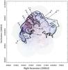 |
Fig. 1 Sample regions from the 35-regions case whose sizes and shapes were obtained with our “feature-tailored” technique. This figure shows the regions (black contours) and their corresponding identification numbers over the 0.3−8.0 keV image. |
For a given mesh, and per region, we extracted spectra from all overlapping observations and created the respective response files for each such spectrum. Background spectra were obtained from source free regions within the respective observations, or, when no such regions were available, from background templates scaled for exposure time.
The brightest X-ray regions in Puppis A (#0 and #1 in the 35-regions case) are prone to suffer from pile-up. In these cases, we removed the EPIC-pn, full window mode spectra from the fits. We rebinned the spectra to a minimum of 20 counts per bin and then fit, per region, a model consisting of an absorbed, plane-parallel shocked plasma with variable abundances (vpshock; Borkowski et al. 2001, and references therein). We used version 2.0 of vpshock, which utilizes atomic data from ATOMDB (Foster et al. 2012). Abundances of elements with prominent lines in the 0.3−8.0 keV band such as O, Ne, Mg, Si, S, and Fe were allowed to vary during the fit while C, N, Ar, Ca and Ni were fixed at the solar value (relative to the solar abundances derived by Anders & Grevesse 1989). Interstellar medium absorption was accounted for with the Tuebingen-Boulder absorption model (tbabs), with abundances set to wilm (Wilms et al. 2000). The fitting was performed with the ISIS spectral analysis package (Houck & Denicola 2000).
In general, all available spectra pertaining to a given region were fit simultaneously. However, spectra obtained from data which were extracted from less than 80% of the area of the data with largest spatial extent were not included; this is to avoid combining spectra taken from disparate areas within one region (an issue which may especially affect the larger regions). Moreover, in those regions which contain both XMM-Newton and Chandra data, the respective EPIC and ACIS spectra were fit with the same spectral model but separately as combined fits did not generally yield acceptable results. For the spectra included in the simultaneous fit, all model parameters were tied, except for independent overall normalizations which were left to vary freely in order to account for differing spatial coverage due to observation dependent instrumental features such as CCD edges, bad pixels and chip gaps.
Comparing the three montage sets, the quality of the spectral fits in terms of  tends to be worse in the 35 and 96 region sets than in the 419 region set. This is to be expected, as the former consists of coarser and larger regions which are more likely to straddle two or more distinct observational fields-of-view, and which, moreover, contain a large number of counts. Therefore, any calibration uncertainties in telescope vignetting and effective area would be more apparent in the resulting fits. In addition, physical properties varying within large regions may also yield worse fits given the model used. Whereas a single temperature model suffices for the finer patchwork, the larger regions may require more complex models. In fact, spectral fits of large regions improve significantly in terms of when, for example, an absorbed two-temperatures shocked plasma is applied. For those regions where the spectral fit yielded
  2, we mitigated the effect of the calibration uncertainties by imposing a stricter minimum coverage fraction, thus restricting the number of simultaneously fit spectra to those of greatest area coverage. A subsequent fit on this reduced data set would in general yield
  2.
2.
3. Results
We perfomed the first complete X-ray analysis of Puppis A. As an example of the power of the method we include here the complete list of fit parameters for the 35-regions case (Table A.1) and show maps of the spatial distribution of NH, kT, O abundance and model normalization (proportional to the plasma emission measure, ∫nenHdV, where ne and nH are the electron and hydrogen densities respectively). Global conclusions, however, are drawn from the precisely fit 419-regions set. Due to the difficulty that represents in practice the labelling of 96 and/or 419 individual regions on an image, the derived parameters are not presented here, but are available upon request to the authors. Here we present the general and more interesting results that confirm the accuracy of our method (see Figs. 1−3).
The method allows extraction of spectral information from the filamentary structures that are evident in the X-ray images. A similar analysis would otherwise require a careful manual definition and selection of those regions. A sample spectrum, from the BEK, is displayed in Fig. 4 together with the fit residuals in sigma units. The spectral model, an absorbed (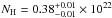 cm-2) single-temperature (
 keV) plasma yields a moderate fit statistic (
 with 1989 degrees of freedom, d.o.f). The fit improves significantly if we add a second plasma to the model (
 /1965 d.o.f., F-test probability < 1-10). This region has been thoroughly studied by Hwang et al. (2005) using observations obtained with Chandra and dividing the BEK into three main morphological components: a bright compact knot, a vertical curved structure (the bar) and a smaller bright cloud (the cap). On average, these regions were found to have temperatures in the 0.3–0.8 keV range and absorption columns in the 0.2–0.5 × 1022 cm-2 range. Our method easily selects all these features as a single region (in the case of 35 regions) finding completely commensurate results.
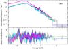 |
Fig. 4 Sample spectra from the region known as BEK towards the eastern edge of Puppis A, arising from the interaction of the SNR shock wave and a molecular cloud. Magenta and black data are from the XMM-Newton PN camera while blue, cyan, yellow, red, and green are data from the MOS camera. The resulting parameters from our fit of the whole region agree with average results obtained by Hwang et al. (2005) from a highly detailed, spatially resolved study using Chandra observations. |
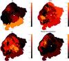 |
Fig. 5 Sample color-coded maps of the spatial distribution of the parameters from the spectral fits. From left to right, this figure shows the spatial distribution of the shock temperature, kT, NH, O/O⊙ abundance, and vpshock normalization (proportional to the plasma emission measure, ∫nenHdV, where ne and nH are the electron and hydrogen densities, respectively). |
The spectra from most regions are of sufficiently high quality to allow us to constrain the elemental abundances. The spatial distribution of O, Ne, Mg, Si, and Fe is mostly smooth with average and standard deviation (weighted by the count rate per region) across the remnant of O/O⊙ = 0.20 ± 0.01, Ne/Ne⊙ = 0.39 ± 0.03, Mg/Mg⊙ = 0.27 ± 0.01, Si/Si⊙ = 0.37 ± 0.07, S/S⊙ = 0.78 ± 2.28, and Fe/Fe⊙ = 0.20 ± 0.02. In agreement with the previous analysis by Katsuda et al. (2008), we found that the abundances are mostly subsolar. Katsuda et al. (2008) tied the sulfur abundances to those of silicon; we left both free to vary during the fit, which resulted in average sulfur abundance close to solar, although the dispersion was too large (see Table A.1) to draw meaningful conclusions.
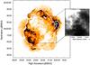 |
Fig. 6 Hardness ratio (0.3−0.7/1.0−8.0 keV) image. The clear stripe crossing the remnant from northeast to southwest follows those regions where the hardness ratio and the intervening absorption column are higher. White contours show the continuum at radio wavelengths that delineate the SNR shock front. The inset shows distribution of NH integrated between 0 and 16.1 km s-1, which is the systemic velocity of Puppis A. The HI data were obtained by Reynoso et al. (2003) (compare with Fig. 3 in D13). |
As shown in Fig. 3, in the 35-regions case, the weak and diffuse X-ray emission toward the recently observed south and southwest portions of Puppis A was selected by our algorithm as a single region (region # 34). The spectrum from this region is well described by a single-temperature shocked plasma with  keV, and abundances of O = 0.28
 , Ne = 0.49
 , Mg = 0.20
 , Si = 0.37
 , S = 2.24
 , and Fe = 0.20. Interestingly, we also found an enhancement of absorption towards this region (see Fig. 5) with a value of
  cm-2 (the average NH across the whole remnant is 0.31 × 1022 cm-2). Figure 6 shows a comparison of the hardness ratio (0.3−0.7)/(1.0−8.0 keV) with the distribution of the absorbing column of atomic gas (as taken from D13), where it can be easily appreciated that the regions where the hardness ratio is higher have a good spatial concordance with the zones having higher NH. As kT tends to be larger towards the center of the SNR, temperature effects can also influence the hardness in the inner portions of the remnant.
The broadband X-ray image from Puppis A reveals a very structured SNR with short curved filaments, suggesting that it is evolving in a complex environment. It is interesting to note that although the brightness morphology is intricate, the spatial distribution of plasma temperature, abundances, and absorption is smooth. The plot of region brightness versus region temperature (Fig. 7) confirms that although there is a wide range of brightness values in Puppis A, in agreement with its filamentary nature, there are no significant temperature changes across the remnant. This finding suggests that the curved structures must be shaped by environmental inhomogeneities encountered by the shock that do not strongly affect the plasma temperature.
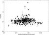 |
Fig. 7 Shock temperature versus surface brightness in the 419-region case. While surface brightness varies over three orders of magnitudes throughout the remnant, the temperature changes by less than a factor of three. |
4. Conclusions
Our distinct technique is designed to extract spectral information from filamentary structures in extended X-ray sources, selecting them by their surface brightness, especially adequate for cases where different instruments are combined. As the spatial
resolution can be tuned by using different bin sizes, the spectral analysis will accordingly reach that level of detail. A big, middle-aged SNR that is rich in structure and that has been observed with different instrumental configurations throughout years, such as Puppis A, represents an excellent pilot case to test this innovative technique to analyze the X-ray spectra along interesting features making it an excellent tool for X-ray studies of extended sources. Future work will include the application of this “feature-tailored” selection of spectral regions to bright, young, ejecta-dominated SNRs.
Acknowledgments
We acknowledge the anonymous referee for the useful comments that helped to improve the quality of this manuscript. G.D., E.G., and G.C. acknowledge support from Argentina grants ANPCYT-PICT 2013-0902, ANPCYT-PICT 0571/11, and CONICET (Argentina) grant PIP 0736/11. G.L., G.D., E.G., and G.C. are members of the “Carrera del Investigador Científico (CIC)” of CONICET.
References
- Anders, E., & Grevesse, N. 1989, Geochim. Cosmochim. Acta, 53, 197 [Google Scholar]
- Aschenbach, B. 1993, Adv. Space Res, 13, 45 [Google Scholar]
- Borkowski, K. J., Lyerly, W. J., & Reynolds, S. P. 2001, ApJ, 548, 820 [NASA ADS] [CrossRef] [Google Scholar]
- Cassam-Chenaï, G., Decourchelle, A., Ballet, J., et al. 2004, A&A, 427, 199 [NASA ADS] [CrossRef] [EDP Sciences] [Google Scholar]
- Dubner, G., Loiseau, N., Rodríguez-Pascual, P., et al. 2013, A&A, 555, A9 [NASA ADS] [CrossRef] [EDP Sciences] [Google Scholar]
- Gaensler, B. M., Arons, J., Kaspi, V. M., et al. 2002, ApJ, 569, 878 [CrossRef] [Google Scholar]
- Güdel, M., Skinner, S. L., Audard, M., Briggs, K. R., & Cabrit, S. 2008, A&A, 478, 797 [NASA ADS] [CrossRef] [EDP Sciences] [Google Scholar]
- Houck, J. C., & Denicola, L. A. 2000, in Astronomical Data Analysis Software and Systems IX, eds. N. Manset, C. Veillet, & D. Crabtree, ASP Conf. Ser., 216, 591 [Google Scholar]
- Hui, C. Y., & Becker, W. 2006, A&A, 457, L33 [NASA ADS] [CrossRef] [EDP Sciences] [Google Scholar]
- Hwang, U., & Laming, J. M. 2012, ApJ, 746, 130 [NASA ADS] [CrossRef] [Google Scholar]
- Hwang, U., Flanagan, K. A., & Petre, R. 2005, ApJ, 635, 355 [NASA ADS] [CrossRef] [Google Scholar]
- Hwang, U., Petre, R., & Flanagan, K. A. 2008, ApJ, 676, 378 [NASA ADS] [CrossRef] [Google Scholar]
- Katsuda, S., Mori, K., Tsunemi, H., et al. 2008, ApJ, 678, 297 [NASA ADS] [CrossRef] [Google Scholar]
- Katsuda, S., Hwang, U., Petre, R., et al. 2010, ApJ, 714, 1725 [NASA ADS] [CrossRef] [Google Scholar]
- Katsuda, S., Tsunemi, H., Mori, K., et al. 2012, ApJ, 756, 49 [NASA ADS] [CrossRef] [Google Scholar]
- Li, J.-T., Decourchelle, A., Miceli, M., Vink, J., & Bocchino, F. 2015, MNRAS, 453, 3954 [Google Scholar]
- Luna, G. J. M., Montez, R., Sokoloski, J. L., Mukai, K., & Kastner, J. H. 2009, ApJ, 707, 1168 [NASA ADS] [CrossRef] [Google Scholar]
- Petre, R., Kriss, G. A., Winkler, P. F., & Canizares, C. R. 1982, ApJ, 258, 22 [NASA ADS] [CrossRef] [Google Scholar]
- Reynoso, E. M., Green, A. J., Johnston, S., et al. 2003, MNRAS, 345, 671 [NASA ADS] [CrossRef] [Google Scholar]
- Sanders, J. S., Fabian, A. C., Churazov, E., et al. 2013, Science, 341, 1365 [Google Scholar]
- Takei, D., Drake, J. J., Yamaguchi, H., et al. 2015, ApJ, 801, 92 [NASA ADS] [CrossRef] [Google Scholar]
- Wilms, J., Allen, A., & McCray, R. 2000, ApJ, 542, 914 [NASA ADS] [CrossRef] [Google Scholar]
Appendix A: Appendix A
Resulting parameters from the fit of an absorbed, plane-parallel shock model with variable abundances to the 35 regions selected with our feature-tailored technique with a count threshold per region of 2 × 10⁶ counts.
All Tables
Resulting parameters from the fit of an absorbed, plane-parallel shock model with variable abundances to the 35 regions selected with our feature-tailored technique with a count threshold per region of 2 × 10⁶ counts.
All Figures
|
Fig. 1 Sample regions from the 35-regions case whose sizes and shapes were obtained with our “feature-tailored” technique. This figure shows the regions (black contours) and their corresponding identification numbers over the 0.3−8.0 keV image. |
| In the text | |
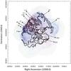 |
Fig. 2 Same as Fig. 1. |
| In the text | |
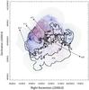 |
Fig. 3 Same as Fig. 1. |
| In the text | |
|
Fig. 4 Sample spectra from the region known as BEK towards the eastern edge of Puppis A, arising from the interaction of the SNR shock wave and a molecular cloud. Magenta and black data are from the XMM-Newton PN camera while blue, cyan, yellow, red, and green are data from the MOS camera. The resulting parameters from our fit of the whole region agree with average results obtained by Hwang et al. (2005) from a highly detailed, spatially resolved study using Chandra observations. |
| In the text | |
|
Fig. 5 Sample color-coded maps of the spatial distribution of the parameters from the spectral fits. From left to right, this figure shows the spatial distribution of the shock temperature, kT, NH, O/O⊙ abundance, and vpshock normalization (proportional to the plasma emission measure, ∫nenHdV, where ne and nH are the electron and hydrogen densities, respectively). |
| In the text | |
|
Fig. 6 Hardness ratio (0.3−0.7/1.0−8.0 keV) image. The clear stripe crossing the remnant from northeast to southwest follows those regions where the hardness ratio and the intervening absorption column are higher. White contours show the continuum at radio wavelengths that delineate the SNR shock front. The inset shows distribution of NH integrated between 0 and 16.1 km s-1, which is the systemic velocity of Puppis A. The HI data were obtained by Reynoso et al. (2003) (compare with Fig. 3 in D13). |
| In the text | |
|
Fig. 7 Shock temperature versus surface brightness in the 419-region case. While surface brightness varies over three orders of magnitudes throughout the remnant, the temperature changes by less than a factor of three. |
| In the text | |
Current usage metrics show cumulative count of Article Views (full-text article views including HTML views, PDF and ePub downloads, according to the available data) and Abstracts Views on Vision4Press platform.
Data correspond to usage on the plateform after 2015. The current usage metrics is available 48-96 hours after online publication and is updated daily on week days.
Initial download of the metrics may take a while.