| Issue |
A&A
Volume 590, June 2016
|
|
|---|---|---|
| Article Number | A112 | |
| Number of page(s) | 12 | |
| Section | Planets and planetary systems | |
| DOI | https://doi.org/10.1051/0004-6361/201526357 | |
| Published online | 25 May 2016 | |
Kepler-539: A young extrasolar system with two giant planets on wide orbits and in gravitational interaction⋆
1 Max-Planck Institute for Astronomy, Königstuhl 17, 69117 Heidelberg, Germany
e-mail: This email address is being protected from spambots. You need JavaScript enabled to view it.
2 INAF–Osservatorio Astrofisico di Torino, via Osservatorio 20, 10025 Pino Torinese, Italy
3 Depto. de Astrofísica, Centro de Astrobiologìa (CSIC-INTA), ESAC campus, 28691 Villanueva de la Cañada, Spain
4 European Southern Observatory, Alonso de Cordova 3107, Vitacura, Casilla 19001, Santiago de Chile, Chile
5 Astrophysics Group, Keele University, Keele ST5 5BG, UK
6 Dip. di Fisica e Astronomia “Galileo Galilei”, Università di Padova, Vicolo dell’Osservatorio 2, 35122 Padova, Italy
7 Dip. di Fisica, Università di Torino, via P. Giuria 1, 10125 Torino, Italy
8 Landessternwarte Königstuhl, Zentrum für Astronomie der Universität Heidelberg, Königstuhl 12, 69117 Heidelberg, Germany
9 Instituto de Astrofísica, Pontificia Universidad Católica de Chile, Av. Vicuña Mackenna 4860, 7820436 Macul, Santiago, Chile
10 Millennium Institute of Astrophysics, Av. Vicuña Mackenna 4860, 7820436 Macul, Santiago, Chile
Received: 19 April 2015
Accepted: 19 April 2016
Abstract
We confirm the planetary nature of Kepler-539 b (aka Kepler object of interest K00372.01), a giant transiting exoplanet orbiting a solar-analogue G2 V star. The mass of Kepler-539 b was accurately derived thanks to a series of precise radial velocity measurements obtained with the CAFE spectrograph mounted on the CAHA 2.2-m telescope. A simultaneous fit of the radial-velocity data and Kepler photometry revealed that Kepler-539 b is a dense Jupiter-like planet with a mass of Mp = 0.97 ± 0.29 MJup and a radius of Rp = 0.747 ± 0.018 RJup, making a complete circular revolution around its parent star in 125.6 days. The semi-major axis of the orbit is roughly 0.5 au, implying that the planet is at ≈0.45 au from the habitable zone. By analysing the mid-transit times of the 12 transit events of Kepler-539 b recorded by the Kepler spacecraft, we found a clear modulated transit time variation (TTV), which is attributable to the presence of a planet c in a wider orbit. The few timings available do not allow us to precisely estimate the properties of Kepler-539 c and our analysis suggests that it has a mass between 1.2 and 3.6 MJup, revolving on a very eccentric orbit (0.4 <e ≤ 0.6) with a period larger than 1000 days. The high eccentricity of planet c is the probable cause of the TTV modulation of planet b. The analysis of the CAFE spectra revealed a relatively high photospheric lithium content, A(Li) = 2.48 ± 0.12 dex, which, together with both a gyrochronological and isochronal analysis, suggests that the parent star is relatively young.
Key words: planetary systems / stars: fundamental parameters / stars: individual: Kepler-539
RV/BVS measurements are only available at the CDS via anonymous ftp to cdsarc.u-strasbg.fr (130.79.128.5) or via http://cdsarc.u-strasbg.fr/viz-bin/qcat?J/A+A/590/A112
© ESO, 2016
1. Introduction
The transiting extrasolar planet (TEP) population turns out to be the best asset in the hands of exoplanetary scientists. Thanks to the early ground-based systematic surveys (e.g. Bakos et al. 2004, 2013; Alonso et al. 2004; McCullough et al. 2005; Pollacco et al. 2006; Pepper et al. 2007; Alsubai et al. 2013) and surveys from space (CoRoT: Barge et al. 2008, Kepler: Borucki et al. 2011), more than 1290 transiting planetary systems have now been found. The possibility of deriving most of their physical and orbital parameters easily, and even investigating the composition of their atmosphere, make the TEPs the most suitable targets to detect and study in detail. They currently represent the best statistical sample to constrain the theoretical models of planetary formation and evolution. Moreover, transit time variation (TTV) studies permitted the detection of additional non-transiting bodies in many TEP systems, highlighting the great efficacy of high-precision and high-cadence photometry in the search for extrasolar planets.
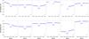 |
Fig. 1 Twelve transit events of Kepler-539 b observed by Kepler in long-cadence mode. The transits at epoch –5 and 2 are clearly affected by starspot-crossing events. Times are in BKJD (equivalent to BJD(TDB) minus 2 454 833.0). |
The majority of TEPs were discovered by the Kepler space telescope, which has revealed how varied they are in terms of mass and size and how diverse their architecture can be. These discoveries have confirmed science fiction images in several cases or and going beyond human imagination in others. The numerous TEP discoveries achieved by Kepler are based on time-series photometric monitoring of the brightness of over 145 000 main-sequence stars in which the periodic-dimming signal caused by a TEP can be found. However, such a signal can be mimic by other astrophysical objects in particular configurations. Radial velocity (RV) follow-up observations of the “potential” parent stars are therefore a fundamental step for distinguishing real TEPs from false positive cases.
Here we focus our attention on the Kepler system Kepler-539. As a result of precise RV measurements, presented in Sect. 2, we confirm the planetary nature of Kepler-539 b (aka KOI-372 b, K00372.01, KIC 6471021), a dense gas-giant planet moving on a wide orbit around a young and active G2 V star (V = 12.6 mag). The analysis of the physical parameters of Kepler-539 b and its parent star are described in Sect. 3. Moreover, the clear variation observed in the mid-time transits of Kepler-539 b strongly support the existence of an additional massive planet, Kepler-539 c, in the system, moving on a larger and very eccentric orbit, as discussed in Sect. 4. We summarise our results in Sect. 5.
2. Observations and data analysis
2.1. Kepler photometry
The Kepler spacecraft monitored Kepler-539 from quarters 0 to 17 (i.e. four years; from May 2009 to May 2013). It was labelled as a Kepler object of interest (KOI) because of a ~0.8% dimming in its light curve with a period of ~125 days (Borucki et al. 2011). This periodic dimming is actually caused by the transit of a Jupiter-like planet candidate, Kepler-539 b, moving on a wide orbit around the star. Twelve transits of Kepler-539 b are present in the Kepler long-cadence (LC) light curves. We labelled these transits from cycle –5 to cycle 6 (see Fig. 1). Two of the transits are incomplete (cycles –2 and –1); two are most likely contaminated by starspot crossing anomalies (cycles –5 and 2); three were also covered in short cadence (SC) (cycles 4, 5, and 6; see Fig. 2). The complete Kepler light curve is shown in Fig. 3, which highlights a significant stellar variability (0.0470 ± 0.0002 mag peak-to-peak). McQuillan et al. (2013) found a periodic photometric modulation in the light curve and, by assuming that it is induced by starspot activity, estimated a stellar rotation period of 11.769 ± 0.016 days. This value is in good agreement with that found by Walkowicz & Basri (2013a,b), i.e. 11.90 ± 3.45 days.
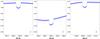 |
Fig. 2 Three transit events of Kepler-539 b observed by Kepler in short-cadence mode. Times are in BKJD (equivalent to BJD(TDB) minus 2 454 833.0). |
 |
Fig. 3 Entire Kepler light-curve data of Kepler-539. The large stellar variability can be reasonable interpreted as induced by a starspot activity. Times are in BKJD (equivalent to BJD(TDB) minus 2 454 833.0). The red arrows indicate the mid-times of the 12 transits of Kepler-539 b. |
2.2. Radial velocity follow-up observations
We monitored Kepler-539 between July 2012 and July 2015 with the Calar Alto Fibre-fed Echelle spectrograph (CAFE; Aceituno et al. 2013) mounted on the 2.2 m telescope at the Calar Alto Observatory (Almería, Spain) as part of our follow-up programme of Kepler candidates. This programme has already confirmed the planetary nature of Kepler-91 b (Lillo-Box et al. 2014a,b), Kepler-432 b (Ciceri et al. 2015), Kepler-447 b (Lillo-Box et al. 2015b), and has identified and characterised some false positives in the sample of Kepler planet candidates (Lillo-Box et al. 2015a). The CAFE spectrograph has a spectral coverage from 4000 Å to 9500 Å, divided into 84 orders with a mean resolving power of R = 63 000. We acquired 28 spectra, which were reduced using the dedicated pipeline provided by the observatory (Aceituno et al. 2013). We used thorium-argon (ThAr) exposures obtained after each science spectrum to wavelength calibrate the corresponding data. The final spectra have signal-to-noise ratios (S/N) in the range S/N = 7–16. An RV was obtained from each spectrum by using the cross-correlation technique through a weighted binary mask (Baranne et al. 1996). The mask is composed of more than 2000 sharp and isolated spectral lines in the CAFE wavelength range. The cross correlation was performed in a ±30 km s-1 range around the expected RV of the star. The peak of the cross-correlation function (CCF) was measured by fitting a four-term Gaussian profile. This velocity was then corrected for the barycentric Earth radial velocity at mid-exposure time. Since we took several consecutive spectra on the same nights, we decided to combine the RV values of the corresponding pairs in the cases where their individual S/N was low (i.e. S/N< 10) and mutual discrepancies were larger than 50 m s-1. This procedure can also diminish the effect of short-term variability, such as the granulation noise, on the radial velocity (although here the expected amplitudes are of the order of few tens of m s-1). Some of the spectra were neglected owing to low quality, mainly caused by weather conditions or problems with the stability of the ThAr lamp. We obtained 20 RV values in total which are reported, together with their observing times, in Table 1 and are compatible with the presence of a ~1 MJup planet in the system (see Fig. 7 and Sect. 4).
Radial velocity and BVS measurements of Kepler-539 from CAHA/CAFE.
2.3. Spectral analysis and the age of Kepler-539
We derived the spectroscopic parameters of the host star Kepler-539 from the co-added CAFE spectra, which has a S/N of about 40 per pixel at 5500 Å. Following the procedures described in Gandolfi et al. (2013, 2015), we used a customised IDL1 software suite to fit the composite CAFE spectrum to a grid of synthetic theoretical spectra. These spectra were calculated with the stellar spectral synthesis programme SPECTRUM (Gray & Corbally 1994) using ATLAS9 plane-parallel model atmospheres (Kurucz 1979), under the assumptions of local thermodynamic equilibrium (LTE) and solar atomic abundances as given in Grevesse & Sauval (1998). We fitted spectral features that are sensitive to different photospheric parameters. Briefly, we used the wings of the Balmer lines to estimate the effective temperature Teff of the star, and the Mg i 5167, 5173, and 5184 Å, the Ca i 6162 and 6439 Å, and the Na i D lines to determine the surface gravity log g⋆. The iron abundance [Fe/H] and microturbulent velocity vmicro was derived by applying the method described in Blackwell & Shallis (1979) on isolated Fe i and Fe ii lines. To determine the macroturbulent velocity vmacro, we adopted the calibration equations for solar-like stars from Doyle et al. (2014). The projected rotational velocity v sini⋆ was measured by fitting the profile of several clean and unblended metal lines2. We found that Kepler-539 has an effective temperature of Teff = 5820 ± 80 K, log g⋆ = 4.4 ± 0.1 (cgs), [Fe/H]=−0.01 ± 0.07 dex, vmicro = 1.1 ± 0.1 km s-1, vmacro = 3.2 ± 0.6 km s-1, and v sini⋆ = 4.4 ± 0.5 km s-1 (Table 3). According to the Straizys & Kuriliene (1981) calibration scale for dwarf stars, the effective temperature of Kepler-539 translates to a G2 V spectral type.
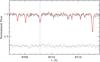 |
Fig. 4 CAFE co-added spectrum of Kepler-539 (black line) encompassing the Li i 6707.8 Å absorption doublet. The best-fitting ATLAS9 spectrum is overplotted with a thick red line. The vertical dashed line indicates the position of the Li doublet. The lowest part of the plot shows the residuals to the fit. |
The CAFE co-added spectrum of Kepler-539 reveals the presence of a moderate Li i 6707.8 Å absorption doublet (Fig. 4). We estimated the photospheric lithium abundance of the star by fitting the Li doublet using ATLAS9 LTE model atmospheres. We fixed the stellar parameters to the values given in Table 3 and allowed our code to fit the lithium content. Adopting a correction for non-LTE effects of +0.006 dex (Lind et al. 2009), we measured a lithium abundance of A(Li) = log (n(Li) /n(H)) + 12 = 2.48 ± 0.12 dex.
The photospheric lithium content and moderate rotation period of Kepler-539 suggest that the star is relatively young. Figure 5 shows the lithium abundance of Kepler-539 compared to the A(Li) of the dwarf stars of the Pleiades, Hyades, and NGC 752 open clusters, as listed in Soderblom et al. (1993), Pace et al. (2012), and Sestito et al. (2004), respectively. Kepler-539 has to be older than ~0.1 Gyr, as the star falls below the envelope of the Pleiades. Although lithium depletion becomes ineffective beyond an age of 1–2 Gyr (Sestito & Randich 2005), Kepler-539 lies between the envelopes of the other two clusters, suggesting an age intermediate between the age of the Hyades (~0.6 Gyr) and NGC 752 (~2.0 Gyr). This is further confirmed by the fact that the lithium content of Kepler-539 is intermediate between the average lithium abundance measured in early G-type stars of 0.6-Gyr open clusters (A(Li) = 2.58 ± 0.15 dex) and that of 2-Gyr open clusters (A(Li) = 2.33 ± 0.17 dex; Sestito & Randich 2005).
We used Eq. (32) from Barnes (2010) and the rotation period of Kepler-539 to infer its gyrochronological age, assuming a convective turnover timescale of τc = 34 days (Barnes & Kim 2010) and a zero-age main-sequence rotation period of P0 = 1.1 days (Barnes 2010). We found a gyrochronological age of 1.0 ± 0.3 Gyr, which supports the relatively young scenario. Our estimation is in good agreement with the 1.15 Gyr gyrochronological age predicted by Walkowicz & Basri (2013a,b) and with that estimated using theoretical models (see Sect. 3 and Table 3).
It is in principle possible to perform an asteroseismic analysis and to try to precisely estimate the age of a star over a very large time span with short-cadence data. However, in the case of Kepler-539, the SC data are only available for less than half the quarters. In particular, the continuous time baseline of SC data is not more than 125 d in the best case (BJD 2 456 015−2 456 139). Furthermore, the activity variation is predominant in the data. We analysed such SC data by filtering the variability due to activity with moving averages, but we did not find evidence of a clear frequency comb in the power spectrum and therefore we did not obtain particular clues about patterns due to solar-like oscillations. We concluded that no reliable asteroseismic analysis could be performed for Kepler-539 based on the Kepler data.
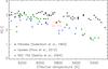 |
Fig. 5 Lithium abundances of F- and G-type dwarf stars in the Pleiades (black dots; Soderblom et al. 1993), Hyades (green squares; Pace et al. 2012), and NGC 752 (blue triangles; Sestito et al. 2004) open clusters. The red dot indicates the position of Kepler-539. |
2.4. Excluding false-positive scenarios
A faint pulsating variable star or a binary system in the background/foreground can mimic a planetary transit signal on the target star. High-resolution images are extremely useful to exclude this possibility (e.g. Lillo-Box et al. 2014c). A Ks-band, high-resolution, adaptive optics image of Kepler-539 was obtained with ARIES on the 6.5 m MMT telescope by Adams et al. (2012), who found four stars within 6′′ of the target; see Table 2. Following Lillo-Box et al. (2012), we estimated the dilution effect caused by each companion, finding that it is very small for the three closest targets, roughly 0.023% in total and thus negligible. The very bright companion “E” is another object targeted as KIC 6471028. As it lies outside the Kepler aperture, this star does not contaminate Kepler-539. KIC 6471028 was also detected with the AstraLux North instrument mounted on the CAHA 2.2 m telescope by Lillo-Box et al. (2012), who estimated that this is a K2-K4 background dwarf.
An intense stellar activity could mimic the presence of a planetary body in the RV signal, thus causing a false positive case. We also analysed such a possibility by determining the bisector velocity span (BVS) from the CAFE spectra (the values are reported in Table 1). The bisector analysis provides a Pearson correlation coefficient between the RV and BVS of  (median value and 95% confidence intervals from the posterior probability distribution; see Figueira et al. 2016). This value indicates only a weak correlation between the two parameters, which is only significant at a 2σ level for the median value and still at less than 3σ for the upper boundary. Consequently, we assume no correlation between both parameters, although we express caution about the weak probability of correlation.
Nearby visual companions around Kepler-539 (from Adams et al. 2012) and their dilution effect on the depth of the transit events.
3. Physical properties of the system
Final parameters of the planetary system KOI-0372.
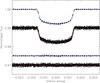 |
Fig. 6 Phased Kepler long-cadence (top light curve) and short-cadence (bottom light curve) data zoomed around transit phase. The TTVs (see Sect. 4) were removed from the data before plotting. The jktebop best fits are shown using solid lines. The residuals of the fits are plotted at the base of the figure. |
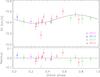 |
Fig. 7 Upper panel: phased RVs for Kepler-539 and the best fit from jktebop. Lower panel: residuals of RVs versus best fit. |
For the determination of the physical parameters of the Kepler-539 system, we proceeded as in Ciceri et al. (2015). We first selected all data within two transit durations of a transit for analysis, ignoring the two with only partial coverage in the Kepler light curve, and converted the units from flux to magnitude. Each transit was then detrended by fitting a polynomial versus time. High polynomial of orders of 3 to 5 were required to account for the brightness variations of the host star caused by spot activity.
We then fitted the photometry and the CAFE RV measurements simultaneously using the jktebop code (Southworth 2013), after modifying it to allow fitting for individual times of mid-transit. The Kepler LC and SC data were fitted separately, accounting for the long effective exposure times in the LC data by oversampling the fitted model by a factor of five.
The following parameters were fitted: the fractional radii of the two objects (r⋆ = R⋆/a and rp = Rp/a, where a is the orbital semi-major axis), the orbital inclination i, the time of midpoint of each transit, the velocity amplitude K⋆, the systemic velocity Vγ, and the coefficients of the polynomial for each transit. The orbital period, Porb, and reference transit midpoint, T0, were fixed to the values measured from the transit times; these were used only for phasing the RV measurements. As in the other papers of our series (e.g. Mancini et al. 2013a,b), a quadratic limb darkening law was used, with the linear term fitted and the quadratic term fixed to 0.27 (Sing 2010). We rescaled the error bars of the LC, SC and RV data to give a reduced χ2 of  for each versus the fitted model. Based on our experience with similar studies (e.g. Mancini et al. 2014a,b), this procedure is necessary for taking underestimated data errors and additional sources of white noise into account; for example an RV jitter due to the activity of the host star.
The best fits to the photometry and RVs are shown in Figs. 6 and 7. The uncertainties in the fitted parameters were derived by running both Monte Carlo and residual-permutation simulations (Southworth 2008) and choosing the larger of the two error bars for each parameter. The results obtained using the SC data are more precise than those from the LC data, so they were adopted as the final set of photometric parameters.
We find that the observations are fully consistent with Kepler-539 b moving on a circular orbit. However, we performed the fit both fixing the orbital eccentricity e to zero and fitting for it via the combination terms ecosω and esinω, where ω is the argument of periastron. In the latter case, we obtained  . We then used the Bayesian information criterion (BIC) to evaluate the preferred scenario, finding that the eccentric case is not favoured over the zero eccentricity model.
Finally, we estimated the age and physical properties of the system from the SC results and the Teff and [Fe/H] measured from our spectra. Constraints from theoretical stellar models were used to make the solution determinate. We followed the HSTEP approach (Southworth 2012, and references therein), which yielded measurements of the properties of the star and planet accompanied by both statistical and systematic error bars. The final results are reported in Table 3.
4. Planet Kepler-539 c from transit time variation
We analysed the 12 mid-transit times of Kepler-539 b to characterise the ephemeris of the transit and check wether there is a possible TTV that could be a sign of the presence of additional bodies in this system. Since the transits at cycles –5 and 2 are somewhat affected by starspots, we used the prism3 and gemc4 codes (Tregloan-Reed et al. 2013, 2015) that allowed us to fit both the full transit events and the shorter starspot-occultation events contemporaneously. The parameters of the starspots coming from the fits are reported in Appendix A. The mid-transit times for the other epochs were estimated using jktebop. The resulting timings are tabulated in Table 4 and were fitted with a straight line to obtain the orbital period, Porb = 125.63243 ± 0.00071 days, and the reference time of mid-transit, T0 = 2 455 588.8710 ± 0.0030 BJD (TDB). A plot of the residuals around the fit (see Fig. 8) shows a clear and modulated deviation from the predicted transit times, meaning that the orbital period of Kepler-539 b is variable (the maximum TTV is 58.5 ± 1.6 min and was measured for the transit at cycle −5). The uncertainties of Porb and T0 were increased to account for this, but we stress that these values should be used with caution as they are based on only 12 timings. Of these timings, two are incomplete and others are affected by starspot anomalies that can introduce offsets in the transit timing measurements; several studies have quantified this effect (e.g. Barros et al. 2013; Oshagh et al. 2013; Mazeh et al. 2015; Ioannidis et al. 2016). We reported the predicted mid-transit times in Table 5 for the next year and a half.
Kepler times of transit midpoint of Kepler-539 b and their residuals.
Future mid-transit times of Kepler-539 b.
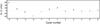 |
Fig. 8 O–C diagram for the timings of Kepler-539 b at mid-transit versus a linear ephemeris. The timings in blue refer to those coming from the Kepler LC data, while those in green are from SC data. The red points refer to the two LC transits affected by starspots. The two incomplete LC transits are indicated with orange points. |
In order to identify the origin of this modulated TTV, we used the TRADES (TRAnsits and Dynamics of Exoplanetary Systems; Borsato et al. 2014) code, which facilitates modelling of the dynamics of multiple-planet systems by reproducing the observed mid-transit times and RVs with the possibility to choose among four different algorithms. We thus investigated the possibility that Kepler-539 is a planetary system formed by a star and two planets, b and c. We ran two series of simulations, the first by selecting the PIKAIA algorithm (Charbonneau 1995), the second with the particle swarm optimization (PSO) algorithm (Tada 2007). In all of the cases, we fixed tight boundaries for the parameters of planet b (centred on the values in Table 3) and assumed the zero eccentricity case, which means that we fixed the argument of pericentre (ωb) to 90°, and let only the mean anomaly (νb) of planet b freely float between 0 and 360 deg. We use a time of reference (or epoch, tepoch = 2 455 463.244) that is very close to the transit cycle 0, forcing the planet b to be initially at the pericentre. Because of this, all of the solutions of both the algorithms returned zero values for νb. Furthermore, for simplicity we assumed the two planets were coplanar. We investigated different configurations of two planet system, with the period of planet c, Pc, varying from 150 to 2500 days. We fitted the pair eccosωc,ecsinωc instead of ec,ωc to avoid correlation between the parameters. We set 0.9 as the highest value allowed for the eccentricity, while we let ωc and νc freely vary as for νb. The solutions obtained from the TRADES fitting processes were further analysed using the frequency map analysis (FMA; Laskar et al. 1992) to check if they are stable.
We found that the best solutions are those related to configurations with Pc> 1000 days and a mass of the planet c between 1.2 and 3.6 MJup on a very eccentric orbit (0.4 <ec ≤ 0.6). The final parameters, with confidence intervals estimated with a bootstrapping method, are reported in Table 6 for the five best solutions based on the χ2 and in the Appendix B figures. The estimated confidence intervals are very tight to the fitted values because the algorithms found solutions that correspond to minimum surrounded by very high peaks in the χ2-space. We also exhaustively investigated a narrow region (200–800 days) of Pc (in steps of about 300 days), but the solutions that we obtained are not favoured because the corresponding χ2 is much higher than those reported in Table 6.
Knowing the orbital period of Kepler-539 c, we can easily estimate the semi-major axis and the equilibrium temperature of the planet c for each solution. These values are shown in right-hand columns of Table 6. Moreover, we can use Eq. (7.29) from Haswell (2010) to estimate the maximum TTV signal expected for Kepler-539 b, i.e.  (1)The last column of Table 6 reports the values of TTVmax for each of the five solutions. The best TRADES solution is also that for which the maximum TTV signal is higher than the others and in better agreement with the observations.
Very interestingly, the high eccentricity of planet c gives a direct explanation of the modulation of the TTV of planet b: when planet c moves close to planet b, it gravitationally kicks its smaller sibling, causing the maximum in the TTV signal; after the conjunction, planet b re-circularises its own orbit very slowly because of tidal interactions with the star and planet c moving far from it. This causes the decreasing of amplitude of its TTV that we see in Fig. 8.
We again stress that all the values presented in Table 6 should be taken with caution, because the existence of planet c can be definitively constrained by new transit observations, able to completely cover the TTV phase of planet b. In particular, one should verify if there is a periodic repetition of the peak and the modulation.
Left-hand columns: parameters of Kepler-539 c from the best fit of the Kepler mid-transit times and CAFE-RV measurements. The best five solutions obtained with TRADES are shown. Left-hand columns: parameters determined from the previous.
5. Discussion and conclusions
Thanks to precise RV measurements obtained with the high-resolution spectrograph CAFE, we confirmed the planetary nature of Kepler-539 b, a dense Jupiter-like planet with a mass of 0.97 ± 0.29 MJup and a radius of 0.747 ± 0.018 RJup, revolving with a period of 125.6 days on a circular orbit around a G2 V star, similar to the Sun. The parameters of the parent star and planet b were obtained by analysing the CAFE spectra and through a joint fit to the RV data and Kepler transit light curves. Orbiting at ~0.5 au from its host, Kepler-539 b is not located too far (≈0.45 au) from its habitable zone (HZ), which has a width of ~0.72 au, as we estimated it based on the stellar parameters reported in Table 3 and the HZ calculator by Kopparapu et al. (2013, 2014). The parent star is quite active, as shown by the 0.047 mag peak-to-peak modulation present in the long time-series photometry and from the starspot anomalies clearly visible in two of the transit events monitored by Kepler. Even though it has physical characteristics that resemble those of the Sun, Kepler-539 is much younger: 1.0 ± 0.3 Gyr as estimated from its lithium abundance and gyrochronology.
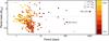 |
Fig. 9 Period–planetary mass diagram for transiting planets in the mass range 0.3 MJup<Mp< 11 MJup. The size of each circle is proportional to the corresponding planetary radius, while the colour indicates equilibrium temperature (data taken from TEPCat). The dashed line demarcates the high-mass regime (Mp> 2MJup). The positions of Kepler-539 b and Kepler-539 c are highlighted. Kepler-539 c is indicated with a box since we do not know its radius. The error bars were suppressed for clarity. |
An analysis of the Kepler mid-transit times of Kepler-539 b revealed a clear modulated TTV signal. We studied this with TRADES, a code that is able to make a simultaneous fit of RV and mid-transit times and compare the results with simulated data of various multi-planetary configurations. We found that the TTV can be explained through the presence of a 1.2–3.6 MJup Jovian-like planet c on a very eccentric (e = 0.43–0.61) and wider orbit than that of Kepler-539 b with a period larger than 1000 days. Each of the five solutions that we presented are related to a planetary system that is stable according to the results of an FMA analysis.
Since the orbit of Kepler-539 c is highly eccentric, then the modulation of the TTV signal of Kepler-539 b can be easily explained. As the distance of planet c from the parent star varies with time, there is a periodic change of the mid-transit time of planet b. In particular, when the planet c is in conjunction with planet b, the gravitational interaction between the two planets is maximum and we see a large amplitude of the TTV signal. Then, when planet c moves away, planet b re-circularises its orbit very slowly and we see the gradual decrease of the amplitude of its TTV.
Given its relatively young age, the physical parameters of the Kepler-539 planetary system can be of great value to astrophysicists working on theories of planet formation and evolution. If we visualise the known transiting planets, reported in TEPCat5, in a period–mass diagram, we can see that Kepler-539 b and Kepler-539 c occupy sparsely populated regions of this plot; here for the mass of Kepler-539 c we considered the best value found by TRADES.
We also underline that the transits of Kepler-539 b are sufficiently deep (0.8%) and that the host star is relatively bright (V = 12.5 mag) and therefore amenable for exoplanet atmosphere studies. The star-planet distance is large enough to consider Kepler-539 b a non-inflated planet with a low irradiation level. Since there are only a handful of transiting Jupiter-like planets with a low irradiation level, this planetary system could be a precious target for future studies of exoplanet atmospheres of normal giant gas planets.
Unfortunately, the parameters of Kepler-539 c are not well constrained as they are based on a poorly sampled TTV (only 12 transit timings). More transits of Kepler-539 b and more precise RV observations from a telescope with a larger-aperture are required to properly model its TTV signal and accurately determine the existence and physical properties of Kepler-539 c on a solid ground. While there are now several high-resolution spectrographs with RV performance better than CAFE, the observations of new transits of Kepler-539 b are not straightforward with ground-based facilities. The 125.6-day orbital period and long transit duration (9.31 h) put serious limitations on the success of a such long-term monitoring and require a large observational effort with various telescopes located at different Earth’s longitudes. Furthermore, in the end, the use of different telescopes could compromise the precision of the measurements of T0. On the other hand, observations of new mid-transit times of Kepler-539 b can be easily performed by the incoming space telescope CHEOPS. This facility is therefore highly recommended for a new detailed follow-up study of the Kepler-539 planetary system.
The acronym IDL stands for Interactive Data Language and is a trademark of ITT Visual Information Solutions.
Here i⋆ refers to the inclination of the stellar rotation axis with respect to the line of sight.
Planetary Retrospective Integrated Starspot Model.
Genetic Evolution Markov Chain.
Transiting Extrasolar Planet Catalogue (TEPcat) is available at http://www.astro.keele.ac.uk/jkt/tepcat/ (Southworth 2011).
Acknowledgments
This paper is based on observations collected with the 2.2 m telescope at the Centro Astronómico Hispano Alemán (CAHA) in Calar Alto (Spain) and the publicly available data obtained with the NASA space satellite Kepler. Operations at the Calar Alto telescopes are jointly performed by the Max-Planck-Institut für Astronomie (MPIA) and the Instituto de Astrofísica de Andalucía (CSIC). This research was partially funded by Spanish grant AYA2012-38897-C02-01. J.L.-B. thanks the CSIC JAE-predoc programme for Ph.D. fellowship support. R.B. is supported by CONICYT-PCHA/Doctorado Nacional. R.B. acknowledges additional support from project IC120009 “Millenium Institute of Astrophysics (MAS)” of the Millennium Science Initiative, Chilean Ministry of Economy. We wish to thank Ennio Poretti for very helpful comments. We acknowledge the use of the following internet-based resources: the ESO Digitized Sky Survey; the TEPCat catalogue; the SIMBAD database operated at CDS, Strasbourg, France; and the arXiv scientific paper preprint service operated by Cornell University.
References
- Aceituno, J., Sãnchez, S. F., Grupp, F., et al. 2013, A&A, 552, A31 [NASA ADS] [CrossRef] [EDP Sciences] [Google Scholar]
- Adams, E. R., Ciardi, D. R., Dupree, A. K., et al. 2012, AJ, 144, 42 [NASA ADS] [CrossRef] [Google Scholar]
- Alonso, R., Brown, T. M., Torres, G., et al. 2004, ApJ, 613, 153 [Google Scholar]
- Alsubai, K. A., Parley, N. R., Bramich, D. M., et al. 2013, AcA, 63, 465 [Google Scholar]
- Bakos, G. Á., Noyes, R. W., Kovács, G., et al. 2004, PASP, 116, 266 [NASA ADS] [CrossRef] [Google Scholar]
- Bakos, G. Á., Csubry, Z., Penev, K., et al. 2013, PASP, 125, 154 [NASA ADS] [CrossRef] [Google Scholar]
- Baranne, A., Queloz, D., Mayor, M., et al. 1996, A&AS, 119, 373 [NASA ADS] [CrossRef] [EDP Sciences] [Google Scholar]
- Barge, P., Baglin, A., Auvergne, M., et al. 2008, A&A, 482, L17 [NASA ADS] [CrossRef] [EDP Sciences] [Google Scholar]
- Barnes, S. A. 2010, ApJ, 722, 222 [NASA ADS] [CrossRef] [Google Scholar]
- Barnes, S. A., & Kim, Y.-C. 2010, ApJ, 721, 675 [NASA ADS] [CrossRef] [Google Scholar]
- Barros, S. C. C., Boué, G., Gibson, N. P., et al. 2013, MNRAS, 430, 3032 [NASA ADS] [CrossRef] [Google Scholar]
- Blackwell, D. E., & Shallis, M. J. 1979, MNRAS, 186, 673 [NASA ADS] [CrossRef] [Google Scholar]
- Borsato, L., Marzari, F., Nascimbeni, V., et al. 2014, A&A, 571, A38 [NASA ADS] [CrossRef] [EDP Sciences] [Google Scholar]
- Borucki, W. J., Koch, D., Basri, G., et al. 2011, ApJ, 736, 19 [NASA ADS] [CrossRef] [Google Scholar]
- Charbonneau, P. 1995, ApJS, 101, 309 [NASA ADS] [CrossRef] [Google Scholar]
- Ciceri, S., Lillo-Box, J., Southworth, J., et al. 2015, A&A, 573, L5 [NASA ADS] [CrossRef] [EDP Sciences] [Google Scholar]
- Doyle, A. P., Davies, G. R., Smalley, B., et al. 2014, MNRAS, 444, 3592 [NASA ADS] [CrossRef] [Google Scholar]
- Figueira, P., Faria, J. P., Adibekyan, V. Z., et al. 2016, Proc. conference Habitability in the Universe: From the Early Earth to Exoplanets [arXiv:1601.05107] [Google Scholar]
- Gandolfi, D., Parviainen, H., Fridlund, M., et al. 2013, A&A, 557, A74 [NASA ADS] [CrossRef] [EDP Sciences] [Google Scholar]
- Gandolfi, D., Parviainen, H., Deeg, H. J., et al. 2015, A&A, 576, A11 [NASA ADS] [CrossRef] [EDP Sciences] [Google Scholar]
- Gray, R. O., & Corbally, C. J. 1994, AJ, 107, 742 [NASA ADS] [CrossRef] [Google Scholar]
- Grevesse, N., & Sauval, A. J. 1998, Space Sci. Rev., 85, 161 [NASA ADS] [CrossRef] [Google Scholar]
- Haswell C. A. 2010, Transiting Exoplanets (Cambridge University Press) [Google Scholar]
- Ioannidis, P., Huber, K. F., & Schmitt, J. H. M. M. 2016, A&A, 585, A72 [NASA ADS] [CrossRef] [EDP Sciences] [Google Scholar]
- Kopparapu, R. K., Ramirez, R., Kasting, J. F., et al. 2013, ApJ, 765, 131 [NASA ADS] [CrossRef] [Google Scholar]
- Kopparapu, R. K., Ramirez, R., SchottelKotte, J., et al. 2014, ApJ, 787, L29 [NASA ADS] [CrossRef] [Google Scholar]
- Kurucz, R. L. 1979, ApJS, 40, 1 [NASA ADS] [CrossRef] [Google Scholar]
- Laskar, J., Froeschlé, C., & Celletti, A. 1992, Phys. D, 56, 253 [CrossRef] [Google Scholar]
- Lillo-Box, J., Barrado, D., & Bouy, H. 2012, A&A, 546, A10 [NASA ADS] [CrossRef] [EDP Sciences] [Google Scholar]
- Lillo-Box, J., Barrado, D., Moya, A., et al. 2014a, A&A, 562, A109 [NASA ADS] [CrossRef] [EDP Sciences] [Google Scholar]
- Lillo-Box, J., Barrado, D., Henning, Th., et al. 2014b, A&A, 568, L1 [NASA ADS] [CrossRef] [EDP Sciences] [Google Scholar]
- Lillo-Box, J., Barrado, D., & Bouy, H. 2014c, A&A, 566, A103 [NASA ADS] [CrossRef] [EDP Sciences] [Google Scholar]
- Lillo-Box, J., Barrado, D., Mancini, L., et al. 2015a, A&A, 576, A88 [NASA ADS] [CrossRef] [EDP Sciences] [Google Scholar]
- Lillo-Box, J., Barrado, D., Santos, N. C., et al. 2015b, A&A, 577, A105 [NASA ADS] [CrossRef] [EDP Sciences] [Google Scholar]
- Lind, K., Asplund, M., & Barklem, P. S. 2009, A&A, 503, 541 [NASA ADS] [CrossRef] [EDP Sciences] [Google Scholar]
- Mancini, L., Southworth, J., Ciceri, S., et al. 2013a, A&A, 551, A11 [NASA ADS] [CrossRef] [EDP Sciences] [Google Scholar]
- Mancini, L., Ciceri, S., Chen, G., et al. 2013b, MNRAS, 436, 2 [NASA ADS] [CrossRef] [Google Scholar]
- Mancini, L., Southworth, J., Ciceri, S., et al. 2014a, A&A, 562, A126 [NASA ADS] [CrossRef] [EDP Sciences] [Google Scholar]
- Mancini, L., Southworth, J., Ciceri, S., et al. 2014b, A&A, 568, A127 [NASA ADS] [CrossRef] [EDP Sciences] [Google Scholar]
- Mazeh, T., Holczer, T., & Shporer, A. 2015, ApJ, 800, 142 [NASA ADS] [CrossRef] [Google Scholar]
- McCullough, P. R., Stys, J. E., Valenti, J. A., et al. 2005, PASP, 117, 783 [NASA ADS] [CrossRef] [Google Scholar]
- McQuillan, A., Mazeh, T., & Aigrain, S. 2013, ApJ, 775, L11 [NASA ADS] [CrossRef] [Google Scholar]
- Oshagh, M., Santos, N. C., Boisse, I., et al. 2013, A&A, 556, A19 [NASA ADS] [CrossRef] [EDP Sciences] [Google Scholar]
- Pace, G., Castro, M., Meléndez, J., et al. 2012, A&A, 541, A150 [NASA ADS] [CrossRef] [EDP Sciences] [Google Scholar]
- Pepper, J., Pogge, R. W., DePoy, D. L., et al. 2007, PASP, 119, 923 [NASA ADS] [CrossRef] [Google Scholar]
- Pollacco, D. L., Skillen, I., Collier Cameron, A., et al. 2006, PASP, 118, 1407 [NASA ADS] [CrossRef] [Google Scholar]
- Sestito, P., & Randich, S. 2005, A&A, 442, 615 [NASA ADS] [CrossRef] [EDP Sciences] [Google Scholar]
- Sestito, P., Randich, S., & Pallavicini, R. 2004, A&A, 426, 809 [NASA ADS] [CrossRef] [EDP Sciences] [Google Scholar]
- Sing, D. 2010, A&A, 510, A21 [Google Scholar]
- Soderblom, D. R., Jones, B. F., Balachandran, S., et al. 1993, AJ, 106, 1059 [NASA ADS] [CrossRef] [Google Scholar]
- Southworth, J. 2008, MNRAS, 386, 1644 [NASA ADS] [CrossRef] [Google Scholar]
- Southworth, J. 2011, MNRAS, 417, 2166 [NASA ADS] [CrossRef] [Google Scholar]
- Southworth, J. 2012, MNRAS, 426, 1291 [NASA ADS] [CrossRef] [Google Scholar]
- Southworth, J. 2013, A&A, 557, A119 [NASA ADS] [CrossRef] [EDP Sciences] [Google Scholar]
- Straizys, V., & Kuriliene, G. 1981, Ap&SS, 80, 353 [NASA ADS] [CrossRef] [Google Scholar]
- Tada, T. 2007, J. Japan Soc. Hydrology Water Resources, 20, 450 [Google Scholar]
- Takeda, Y., Honda, S., Ohnishi, T., et al. 2013, PASJ, 65, 53 [Google Scholar]
- Tregloan-Reed, J., Southworth, J., & Tappert, C. 2013, MNRAS, 428, 3671 [NASA ADS] [CrossRef] [Google Scholar]
- Tregloan-Reed, J., Southworth, J., & Burgdorf, M. 2015, MNRAS, 450, 1760 [NASA ADS] [CrossRef] [Google Scholar]
- Walkowicz, L. M., & Basri, G. S. 2013a, MNRAS, 436, 1883 [NASA ADS] [CrossRef] [Google Scholar]
- Walkowicz, L. M., & Basri, G. S. 2013b, VizieR On-line Data Catalog: J/MNRAS/436/1883 [Google Scholar]
Appendix A: Starspot parameters
In this appendix we report a Table containing the starspot parameters that were determined from the PRISM+GEMC fitting of the transit light curves at cycles −5 and 2, as defined in Sect. 2.1.
Starspot parameters derived from the prism+gemc fitting of the transit light curves at cycles −5 and 2.
Appendix B: TRADES simulations
In this appendix we report plots based on the results of the TRADES simulations for modelling the TTV detected in the transit timings of KOI-327 b. In particular, the figures show RV plots (bottom panels) and O–C diagrams from linear ephemeris for planet Kepler-539 b (top panels). In both cases, the observed data are compared with those obtained from the simulations (see Sect. 4) The figures are ordered as in Table 6. Figures 1, 3 and 4 were obtained using the PIKAIA algorithm (Charbonneau 1995), while Figs. 2 and 5 with the particle swarm optimization (PSO) algorithm (Tada 2007).
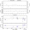 |
Fig. B.1 O–C diagram (with residuals) from linear ephemeris for planet Kepler-539 b (top panel); observations plotted as black points (with error bars) and simulations plotted as open blue circles. Bottom panel shows the RV observations as solid black circles, simulations at the same BJD(UTC) as open blue circles, and the dotted grey line is the RV model for the whole simulation. This the best solution found by trades. |
All Tables
Nearby visual companions around Kepler-539 (from Adams et al. 2012) and their dilution effect on the depth of the transit events.
Left-hand columns: parameters of Kepler-539 c from the best fit of the Kepler mid-transit times and CAFE-RV measurements. The best five solutions obtained with TRADES are shown. Left-hand columns: parameters determined from the previous.
Starspot parameters derived from the prism+gemc fitting of the transit light curves at cycles −5 and 2.
All Figures
|
Fig. 1 Twelve transit events of Kepler-539 b observed by Kepler in long-cadence mode. The transits at epoch –5 and 2 are clearly affected by starspot-crossing events. Times are in BKJD (equivalent to BJD(TDB) minus 2 454 833.0). |
| In the text | |
|
Fig. 2 Three transit events of Kepler-539 b observed by Kepler in short-cadence mode. Times are in BKJD (equivalent to BJD(TDB) minus 2 454 833.0). |
| In the text | |
|
Fig. 3 Entire Kepler light-curve data of Kepler-539. The large stellar variability can be reasonable interpreted as induced by a starspot activity. Times are in BKJD (equivalent to BJD(TDB) minus 2 454 833.0). The red arrows indicate the mid-times of the 12 transits of Kepler-539 b. |
| In the text | |
|
Fig. 4 CAFE co-added spectrum of Kepler-539 (black line) encompassing the Li i 6707.8 Å absorption doublet. The best-fitting ATLAS9 spectrum is overplotted with a thick red line. The vertical dashed line indicates the position of the Li doublet. The lowest part of the plot shows the residuals to the fit. |
| In the text | |
|
Fig. 5 Lithium abundances of F- and G-type dwarf stars in the Pleiades (black dots; Soderblom et al. 1993), Hyades (green squares; Pace et al. 2012), and NGC 752 (blue triangles; Sestito et al. 2004) open clusters. The red dot indicates the position of Kepler-539. |
| In the text | |
|
Fig. 6 Phased Kepler long-cadence (top light curve) and short-cadence (bottom light curve) data zoomed around transit phase. The TTVs (see Sect. 4) were removed from the data before plotting. The jktebop best fits are shown using solid lines. The residuals of the fits are plotted at the base of the figure. |
| In the text | |
|
Fig. 7 Upper panel: phased RVs for Kepler-539 and the best fit from jktebop. Lower panel: residuals of RVs versus best fit. |
| In the text | |
|
Fig. 8 O–C diagram for the timings of Kepler-539 b at mid-transit versus a linear ephemeris. The timings in blue refer to those coming from the Kepler LC data, while those in green are from SC data. The red points refer to the two LC transits affected by starspots. The two incomplete LC transits are indicated with orange points. |
| In the text | |
|
Fig. 9 Period–planetary mass diagram for transiting planets in the mass range 0.3 MJup<Mp< 11 MJup. The size of each circle is proportional to the corresponding planetary radius, while the colour indicates equilibrium temperature (data taken from TEPCat). The dashed line demarcates the high-mass regime (Mp> 2MJup). The positions of Kepler-539 b and Kepler-539 c are highlighted. Kepler-539 c is indicated with a box since we do not know its radius. The error bars were suppressed for clarity. |
| In the text | |
|
Fig. B.1 O–C diagram (with residuals) from linear ephemeris for planet Kepler-539 b (top panel); observations plotted as black points (with error bars) and simulations plotted as open blue circles. Bottom panel shows the RV observations as solid black circles, simulations at the same BJD(UTC) as open blue circles, and the dotted grey line is the RV model for the whole simulation. This the best solution found by trades. |
| In the text | |
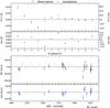 |
Fig. B.2 Same as for Fig. B.1, but showing the 2nd best solution found by trades. |
| In the text | |
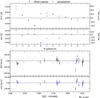 |
Fig. B.3 Same as for Fig. B.1, but showing the 3rd best solution found by trades. |
| In the text | |
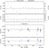 |
Fig. B.4 Same as for Fig. B.1, but showing the 4th best solution found by trades. |
| In the text | |
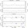 |
Fig. B.5 Same as for Fig. B.1, but showing the 5th best solution found by trades. |
| In the text | |
Current usage metrics show cumulative count of Article Views (full-text article views including HTML views, PDF and ePub downloads, according to the available data) and Abstracts Views on Vision4Press platform.
Data correspond to usage on the plateform after 2015. The current usage metrics is available 48-96 hours after online publication and is updated daily on week days.
Initial download of the metrics may take a while.