| Issue |
A&A
Volume 589, May 2016
|
|
|---|---|---|
| Article Number | A40 | |
| Number of page(s) | 12 | |
| Section | Stellar structure and evolution | |
| DOI | https://doi.org/10.1051/0004-6361/201527996 | |
| Published online | 12 April 2016 | |
Asteroseismology of the GW Virginis stars SDSS J0349−0059 and VV 47
1
Grupo de Evolución Estelar y Pulsaciones, Facultad de Ciencias Astronómicas
y Geofísicas, Universidad Nacional de La Plata,
Paseo del Bosque s/n,
1900
La Plata,
Argentina
2
Instituto de Astrofísica La Plata, CONICET-UNLP, Paseo del Bosque s/n,
1900
La Plata,
Argentina
e-mail: This email address is being protected from spambots. You need JavaScript enabled to view it.
;
This email address is being protected from spambots. You need JavaScript enabled to view it.
; This email address is being protected from spambots. You need JavaScript enabled to view it.
Received: 17 December 2015
Accepted: 20 February 2016
Abstract
Context. GW Virginis stars are a well-studied class of nonradial g-mode pulsators. SDSS J0349−0059 and VV 47 are two PG 1159 star members of this class of variable stars. SDSS J0349−0059 is an interesting GW Vir star that shows a complete pulsation spectrum that includes rotational splitting of some of its frequencies. VV 47 is a pulsating PG 1159 star surrounded by a planetary nebula. This star is particularly interesting because it exhibits a rich and complex pulsation spectrum.
Aims. We present an asteroseismological study of SDSS J0349−0059 and VV 47 aimed mainly at deriving their total mass on the basis of state-of-the-art PG 1159 evolutionary models.
Methods. We computed adiabatic nonradial g-mode pulsation periods for PG 1159 evolutionary models with stellar masses ranging from 0.515 to 0.741 M⊙, that take into account the complete evolution of the progenitor stars. We first estimated a mean period spacing for both SDSS J0349−0059 and VV 47 and then constrained the stellar mass of these stars by comparing the observed period spacing with the asymptotic period spacing and with the average of the computed period spacings. We also employed the individual observed periods to search for a representative seismological model for each star. Finally, we estimated the rotation period of SDSS J0349−0059.
Results. We found a spectroscopic mass of M⋆ ~ 0.543 M⊙ for SDSS J0349−0059 and M⋆ ~ 0.529 M⊙ for VV 47. By comparing the observed period spacing with the asymptotic period spacing, we obtain M⋆ ~ 0.569 M⊙ for SDSS J0349−0059 and M⋆ ~ 0.523 M⊙ for VV 47. When we compare the observed period spacing with the average of the computed period spacings, we find M⋆ ~ 0.535 M⊙ for SDSS J0349−0059 and M⋆ ~ 0.528 M⊙ for VV 47. Searching for the best period fit, we found for SDSS J0349−0059 an asteroseismological model with M⋆ = 0.542 M⊙ and Teff = 91 255 K. For VV 47, we were unable to find a unique and unambiguous asteroseismological model. Finally, for SDSS J0349−0059, we determined the rotation period to be Prot = 1/Ω ~ 0.407 days.
Conclusions. The results presented in this work constitute a further step in the study of GW Vir stars through asteroseismology in the frame of fully evolutionary models of PG 1159 stars. In particular, the potential of asteroseismology to derive stellar masses of PG 1159 stars with an unprecedented precision is shown yet again.
Key words: stars: evolution / stars: interiors / stars: oscillations / white dwarfs
© ESO, 2016
1. Introduction
GW Virginis stars include pulsating stars that are characterized into several spectral types (see Quirion et al. 2007). These include PG 1159 stars, which are very hot H-deficient post-asymptotic giant branch (AGB) stars with surface layers rich in He, C, and O (Werner & Herwig 2006; Werner et al. 2014; Werner & Rauch 2015). Pulsating PG 1159 stars exhibit multiperiodic luminosity variations with periods ranging from 5 to 100 min; the variations are attributable to non-radial pulsation g-modes. Some GW Vir are still embedded in a nebula (see the reviews by Winget & Kepler 2008; Fontaine & Brassard 2008; Althaus et al. 2010)1. PG 1159 stars are thought to be the evolutionary link between Wolf-Rayet-type central stars of planetary nebulae and most of the H-deficient white dwarfs (Wesemael et al. 1985; Sion 1986; Althaus et al. 2005). It is generally accepted that these stars originate in a born-again episode induced by a post-AGB He thermal pulse, see Iben et al. (1983), Herwig et al. (1999), Lawlor & MacDonald (2003), Althaus et al. (2005), Miller Bertolami & Althaus (2006) for references.
Notably, considerable observational effort has been invested to study GW Vir stars. Particularly noteworthy are the works of Vauclair et al. (2002) on RX J2117.1+3412, Fu et al. (2007) on PG 0122+200, and Costa et al. (2008) and Costa & Kepler (2008) on PG 1159−035. On the theoretical front, important progress in the numerical modeling of PG 1159 stars (Althaus et al. 2005; Miller Bertolami & Althaus 2006, 2007a,b) has paved the way for unprecedented asteroseismological inferences for the mentioned stars (Córsico et al. 2007a,b, 2008), and also for PG 2131+066, PG 1707+427, NGC 1501, and SDSS J0754+0852 (Córsico et al. 2009a; Kepler et al. 2014). The detailed PG 1159 stellar models of Miller Bertolami & Althaus (2006) were derived from the complete evolutionary history of progenitor stars with different stellar masses and an elaborate treatment of the mixing and extra-mixing processes during the core He burning and born-again phases. It is worth mentioning that these models are characterized by thick helium-rich outer envelopes. The reliability of the H-deficient post-AGB tracks of Miller Bertolami & Althaus (2006) regarding the previous evolution of their progenitor stars and the constitutive physics of the remnants have been assesed by Miller Bertolami & Althaus (2007a). The success of these models at explaining the spread in surface chemical composition observed in PG 1159 stars (Miller Bertolami & Althaus 2006), the short born-again times of V4334 Sgr (Miller Bertolami & Althaus 2007b), and the location of the GW Vir instability strip in the log Teff −log g plane (Córsico et al. 2006) renders inferences drawn for individual pulsating PG 1159 stars reliable. In the context of nonadiabatic analysis of GW Vir stars, the important theoretical work of Quirion et al. (2004, 2005, 2007, 2012) deserves special mention. These studies have shed light on the questions of variable and non-variable stars in the GW Vir region of the HR diagram and on the existence of the high-gravity red edge of the GW Vir instability domain.
SDSS J0349−0059 is a pulsating PG 1159 star with Teff = 90 000 ± 900 K and log g = 7.5 ± 0.01 (cgs) according to Hügelmeyer et al. (2006), who employed the Data Release 4 of the SDSS Catalog to estimate these quantities using non-local thermodynamic equilibrium (non-LTE) model atmospheres. Woudt et al. (2012) performed high-speed photometric observations in 2007 and 2009 and found a set of pulsation frequencies in the range of 1038–3323 μHz with amplitudes between 3.5 and 18.6 mmag. The data gathered by Woudt et al. (2012) show three frequencies closely spaced in the 2007 data, which in principle enables estimating a period rotation for this star.
VV 47 is a PNNV star characterized by Teff = 130 000 ± 13 000 K and log g = 7 ± 0.5 (Werner & Herwig 2006). Its stellar mass is M⋆ = 0.59 M⊙ according to Werner & Herwig (2006) and M⋆ = 0.53 M⊙ according to the evolutionary tracks created by Miller Bertolami & Althaus (2006). The surface chemical composition of VV 47 is typical of PG 1159 stars: C/He = 1.5 and O/He = 0.4 (Werner & Herwig 2006). VV 47 was first observed as potentially variable by Liebert et al. (1988). Later, it was monitored by Ciardullo & Bond (1996), but no clear variability was found. Finally, González Pérez et al. (2006) were able to confirm the elusive intrinsic variability of VV 47 for the first time. They found clear evidence that the pulsation spectrum of this star is extremely complex. The amplitudes of the main peaks of the power spectrum are strongly variable between observation seasons, and sometimes they are detected only in a particular run. It is apparent that real periodicities of VV 47 are in the range 131−5682 s. The shortest periods in the observed period spectrum of VV 47 could be associated with the ε-mechanism of mode driving acting at the He burning shell, as suggested by González Pérez et al. (2006). This hypothesis was explored from a theoretical point of view by Córsico et al. (2009b). If this hypothesis were confirmed, this object could be the first known pulsating PG 1159 star undergoing pulsation modes powered by this mechanism.
In this work, we present an adiabatic asteroseismological study of SDSS J0349−0059 and VV 47 aimed at determining the internal structure and evolutionary status of these stars on the basis of the very detailed PG 1159 evolutionary models of Miller Bertolami & Althaus (2006). We emphasize that the results presented in this work could change to some extent if another independent set of PG 1159 evolutionary tracks that is constructed assuming a different input physics were employed. We compute adiabatic g-mode pulsation periods on PG 1159 evolutionary models with stellar masses ranging from 0.515 to 0.741 M⊙. These models take into account the complete evolution of progenitor stars through the thermally pulsing AGB phase and born-again episode. A brief summary of the stellar models employed is provided in Sect. 2. We estimate a mean period spacing for both SDSS J0349−0059 and VV 47 (Sect. 3) and then constrain the stellar masses of these stars by comparing the observed period spacing with the asymptotic period spacing and with the average of the computed period spacings (Sect. 4). In Sect. 5 we employ the individual observed periods to search for a representative seismological model for these stars. In Sect. 6 we estimate the rotation period for SDSS J0349−0059, employing the observed triplet of frequencies. Finally, we close the article with a discussion and summary in Sect. 7.
2. Evolutionary models and numerical tools
The pulsation analysis presented in this work relies on a suite of state-of-the-art stellar models that take into account the complete evolution of the PG 1159 progenitor stars. Specifically, the stellar models were extracted from the evolutionary calculations presented by Althaus et al. (2005), Miller Bertolami & Althaus (2006), and Córsico et al. (2006), who computed the complete evolution of model star sequences with initial masses on the ZAMS in the range 1−3.75 M⊙. All of the post-AGB evolutionary sequences computed with the LPCODE evolutionary code (Althaus et al. 2005) were followed through the very late thermal pulse (VLTP) and the resulting born-again episode that give rise to the H-deficient, He-, C-, and O-rich composition characteristic of PG 1159 stars. The masses of the resulting remnants are 0.530, 0.542, 0.565, 0.589, 0.609, 0.664, and 0.741 M⊙. An additional evolutionary track of a remnant with a stellar mass of 0.515 M⊙ is also employed for VV 47. In Fig. 1 the evolutionary tracks are shown in the log Teff−log g plane. The blue and red edges of the theoretical GW Vir instability domain according to Córsico et al. (2006) correspond to PG 1159 models with surface fractional abundances (Xi) of 4He in the range 0.28−0.48, 12C in the range 0.27−0.41 and 16O in the range 0.10−0.23 (see Table 1 of Córsico et al. 2006). For details about the input physics and evolutionary code and the numerical simulations performed to obtain the PG 1159 evolutionary sequences employed here, we refer to Althaus et al. (2005) and Miller Bertolami & Althaus (2006, 2007a,b).
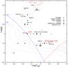 |
Fig. 1 PG 1159 (VLTP) evolutionary tracks of Miller Bertolami & Althaus (2006; from right to left: M⋆ = 0.515, 0.530, 0.542, 0.565, 0.589, 0.609, 0.664, 0.741 M⊙) in the log Teff − log g diagram (thin dotted curves). The location of all known PG 1159 stars (variable, non-variable, and objects with no variability data) is shown, including SDSS J0349−0059 and VV 47 with their uncertainties. The uncertainty values for SDSS J0349−0059 are very low in the adopted scale and are not visible in the plot. The hot blue edges (blue curves) and the low-gravity red edges (upper red curves) of the theoretical GW Vir instability strip for ℓ = 1 (dashed) and ℓ = 2 (dotted) modes according to Córsico et al. (2006) are also depicted. The high-gravity red edge that is due to the competition of residual stellar winds against the gravitational settling of C and O (Quirion et al. 2012) is also included (lower red solid curve). |
On the basis of the evolutionary tracks presented in Fig. 1, a value for the spectroscopic mass2 of SDSS J0349−0059 and VV 47 can be derived by linear interpolation. For SDSS J0349−0059 we derive a stellar mass of M⋆ = 0.543 ± 0.004 M⊙. This is the first time that a mass determination has been made for this star. The uncertainties in log g and log Teff for VV 47 are so large that the value derived for the spectroscopic mass is inaccurate. In this case, we derive a formal value of M⋆ ~ 0.529 M⊙ (in agreement with the value of M⋆ = 0.53 M⊙ derived by Miller Bertolami & Althaus 2006), although it can be as low as ~0.510 M⊙ or as high as ~0.609 M⊙. Quirion et al. (2009) proposed a novel approach called “non-adiabatic asteroseismology”, which leads to a much more precise surface gravity value for VV 47 of log g = 6.1 ± 0.1. By adopting Teff = 130 000 K and log g = 6.1, our evolutionary tracks predict a spectroscopic mass of ~0.542 M⊙.
We computed ℓ = 1,2g-mode adiabatic pulsation periods in the range 80−6000 s with the adiabatic version of the LP-PUL pulsation code (Córsico & Althaus 2006) and with the same methods as we employed in our previous works3. We analyzed about 4000 PG 1159 models covering a wide range of effective temperatures (5.4 ≳ log Teff ≳ 4.8), luminosities (0 ≲ log (L∗/L⊙) ≲ 4.2), and stellar masses (0.515 ≤ M⋆/M⊙ ≤ 0.741).
3. Estimating a constant period spacing
List of the 13 independent frequencies in the 2007 January data of SDSS J0349−0059 from Woudt et al. (2012).
In the asymptotic limit of high-radial order k, nonradial g modes with the same harmonic degree ℓ are expected to be equally spaced in period (Tassoul 1980): ![Mathematical equation: \begin{equation} \label{eq:spacing} \Delta\Pi^{\rm a}_{\ell}=\Pi_{k+1,\ell}-\Pi_{k,\ell}=\frac{2\pi^2}{\sqrt{\ell(\ell+1)}} \left[\int^{R_{\star}}_0{\frac{N(r)}{r}{\rm d}r}\right]^{-1} , \end{equation}](/articles/aa/full_html/2016/05/aa27996-15/aa27996-15-eq103.png) (1)where N is the Brunt-Väisälä frequency. In principle, the asymptotic period spacing or the average of the period spacings computed from a grid of models with different masses and effective temperatures can be compared with the mean period spacing exhibited by the star, and then the value of the stellar mass can be inferred (Sect. 4). These methods take full advantage of the fact that the period spacing of pulsating PG 1159 stars primarily depends on the stellar mass and only weakly on the luminosity and the He-rich envelope mass fraction, as was first recognized by Kawaler (1986, 1987, 1988, 1990; see also Kawaler & Bradley 1994; Córsico & Althaus 2006). These approaches have been successfully applied in numerous studies of pulsating PG 1159 stars (see, for instance, Córsico et al. 2007a,b, 2008, 2009a). The first step in this process is to obtain a mean uniform period separation underlying the observed periods (if one exists). We searched for a constant period spacing in the data of the stars under analysis by using the Kolmogorov-Smirnov (K-S; see Kawaler 1988), the inverse variance (I-V; see O’Donoghue 1994) and the Fourier transform (F-T; see Handler et al. 1997) significance tests. In the K-S test, the quantity Q is defined as the probability that the observed periods are randomly distributed. Thus, any uniform or at least systematically non-random period spacing in the period spectrum of the star will appear as a minimum in Q. In the I-V test, a maximum of the inverse variance will indicate a constant period spacing. Finally, in the F-T test, we calculate the Fourier transform of a Dirac comb function (created from a set of observed periods), and then we plot the square of the amplitude of the resulting function in terms of the inverse of the frequency. And once again, a maximum in the square of the amplitude will indicate a constant period spacing.
(1)where N is the Brunt-Väisälä frequency. In principle, the asymptotic period spacing or the average of the period spacings computed from a grid of models with different masses and effective temperatures can be compared with the mean period spacing exhibited by the star, and then the value of the stellar mass can be inferred (Sect. 4). These methods take full advantage of the fact that the period spacing of pulsating PG 1159 stars primarily depends on the stellar mass and only weakly on the luminosity and the He-rich envelope mass fraction, as was first recognized by Kawaler (1986, 1987, 1988, 1990; see also Kawaler & Bradley 1994; Córsico & Althaus 2006). These approaches have been successfully applied in numerous studies of pulsating PG 1159 stars (see, for instance, Córsico et al. 2007a,b, 2008, 2009a). The first step in this process is to obtain a mean uniform period separation underlying the observed periods (if one exists). We searched for a constant period spacing in the data of the stars under analysis by using the Kolmogorov-Smirnov (K-S; see Kawaler 1988), the inverse variance (I-V; see O’Donoghue 1994) and the Fourier transform (F-T; see Handler et al. 1997) significance tests. In the K-S test, the quantity Q is defined as the probability that the observed periods are randomly distributed. Thus, any uniform or at least systematically non-random period spacing in the period spectrum of the star will appear as a minimum in Q. In the I-V test, a maximum of the inverse variance will indicate a constant period spacing. Finally, in the F-T test, we calculate the Fourier transform of a Dirac comb function (created from a set of observed periods), and then we plot the square of the amplitude of the resulting function in terms of the inverse of the frequency. And once again, a maximum in the square of the amplitude will indicate a constant period spacing.
3.1. SDSS J0349−0059
We were able to infer an estimate for the period spacing of SDSS J0349−0059 by using the data available in Woudt et al. (2012). In particular, we employed the periods listed in Tables 1 and 2, extracted from Table 2 of Woudt et al. (2012), which correspond to two different observation dates. First, we considered the complete set of periods from both tables. The results of our analysis are shown in Fig. 2. The plot shows evidence of a period spacing at about 23.5 s, but it shows other minima as well, at ~17 s in the three tests. Next, we repeated the analysis for several different sets of data in which we discarded one or two periods, following Woudt et al. (2012). We found an unambiguous indication of a constant period spacing of 23.49 s and also a secondary solution of 16.5 s, as can be seen in Fig. 3, where the periods used are listed in boldface in Tables 1 and 2. We can safely identify the period spacing of 23.49 s with ℓ = 1 modes by comparing with the ℓ = 1 period spacing observed in other GW Vir stars: 21.6 s for RXJ2117+3412 (Vauclair et al. 2002), 22.9 s for PG 0122+200 (Fu et al. 2007), 21.4 s for PG 1159−035 (Costa et al. 2008), 21.6 s for PG 2131+066 (Reed et al. 2000), 23.0 s for PG 1707+427 (Kawaler et al. 2004), and 22.3 s for NGC 1501 (Bond et al. 1996). We also compared this with the asymptotic period spacing of our PG 1159 models. We discarded the second-highest amplitude mode of the 2009 set of modes and the fourth-highest amplitude mode of the 2007 set of 13 modes (i.e., Π = 412.27 s and Π = 517.84 s, respectively) because they did not match the determined period spacing associated with ℓ = 1. We found that they are probably associated with ℓ = 2, and our models predict their theoretical values to be 410.38 s and 518.10 s, respectively. For the fifth-highest amplitude mode of the 2007 set (Π = 353.79 s), our models predict that it is associated with ℓ = 1, but the final result is independent of whether or not it is included in the list of the considered periods.
List of the ten independent frequencies in the 2009 December data of SDSS J0349−0059 from Woudt et al. (2012).
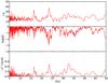 |
Fig. 2 I-V (upper panel), K-S (middle panel), and F-T significance (bottom panel) tests applied to the period spectrum of SDSS J0349−0059 to search for a constant period spacing. The periods used here are those indicated in Table 1 and 2. |
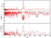 |
Fig. 3 Same as Fig. 2, but for the 15 selected periods of SDSS J0349−0059 emphasized with boldface in Tables 1 and 2. |
When we applied the three significance tests to six of the discarded periods (i.e., 353.79, 412.27, 482.17, 504.18, 516.18, and 517.84 s), we found a period spacing of 11.6 s, as shown in Fig. 4. At this point, we may wonder whether the spacings at 16.5 s and 11.6 s may be associated with ℓ = 2 modes. A simple analysis of the asymptotic period spacing helps us to show that this is not the case. Equation (1) shows that the relation  /
/ between the period spacing corresponding to ℓ = 1 and ℓ = 2 holds. If the period spacing 23.49 s is associated with ℓ = 1, then a
  s should be expected for a period separation associated with ℓ = 2. From this, we conclude that the spacings of 16.5 s and 11.6 s cannot be associated with ℓ = 2 modes.
We refined the value of the period spacing at 23.49 s by performing a least-squares fit to the set of 15 periods employed in building Fig. 3. We obtained ΔΠO = 23.4904 ± 0.07741 s.
From these results we conclude that there exists strong evidence for a constant period spacing of ΔΠO = 23.49 s in the pulsation spectrum exhibited by SDSS J0349−0059. This agrees perfectly well with Woudt et al. (2012). We note that the departures from this period spacing could be associated with mode-trapping or confinement phenomena (Kawaler & Bradley 1994; Córsico & Althaus 2006).
3.2. VV 47
The analysis presented in this section is based on the work of González Pérez et al. (2006). Specifically, we use the periods listed in Table 3, extracted from Table 4 of González Pérez et al. (2006), to estimate a period spacing in VV 47.
Most important peaks in the VV 47 power spectra according to González Pérez et al. (2006).
First, we considered the complete set of periods of Table 3. For simplicity, we adopted a single period of 132.05 s that is the average of the pair of periods at 131.6 s and 132.5 s. The results of our analysis are shown in Fig. 5. In spite of the two minima in log Q (middle panel), they are not statistically meaningful in the context of the K-S test because there are other several minima with similar significance levels. The F-T-based method (lower panel) shows multiple local maxima and is therefore inconclusive. The I-V test (upper panel) does not exhibit any obvious maximum. The application of these tests to the complete list of periods provides no clue about a possible constant period spacing in VV 47.
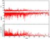 |
Fig. 5 I-V (upper panel), K-S (middle panel), and F-T (bottom panel) significance tests applied to the period spectrum of VV 47 to search for a constant period spacing. The periods used here are those provided by Table 3, where we considered a single period at 132.05 s instead of the pair of periods at 131.6 s and 132.5 s. No unambiguous signal of a constant period spacing is evident. |
Next, we repeated this analysis for numerous different sets of periods, ignoring one or more periods from the list, and then we examined the predictions of the three statistical tests. In particular, we found some evidence of a period spacing of ~24 s when the periods at 132.05 s and 153.5 s were omitted. We also noted that the periods providing the larger discrepancies with this tentative period spacing are 240.4 s, 280.1 s, 3521 s, and 4310 s. Figure 6 is similar to Fig. 5, but it shows the situation in which the periods at 132.05 s, 153.5 s, 240.4 s, 280.1 s, and 3521 s are not taken into account in the analysis. The plot of the remaining 11 periods shows strong evidence of a constant period spacing at 24.2 s in the three tests.
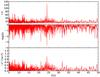 |
Fig. 6 Same as Fig. 5, but discarding the periods at 132.05 s, 153.5 s, 240.4 s, 280.1 s, and 3521 s of VV 47 from the analysis (see text for details). |
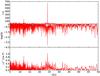 |
Fig. 7 Same as Fig. 5, but discarding the periods at 132.05 s, 153.5 s, 240.4 s, 280.1 s, 3521 s, and 4310 s of VV 47 from the analysis (see text for details). |
To confirm our hypothesized period spacing, we repeated the three tests, but this time by discarding the period at 4310 s as well, which also presents a significant departure from an equally spaced period pattern. We obtained a very strong confirmation for a period spacing of ΔΠO = 24.2 s by using this subset of ten periods. This is illustrated in Fig. 7. The agreement between the three methods is excellent. The K-S test indicates that this constant period spacing is significant at a confidence level of [ 100 × (1−Q) ] = 99%. The F-T also shows unambiguous evidence of this value. However, the clearest and most unambiguous indication of ΔΠO = 24.2 s is provided by the I-V test. It is also possible to visualize the first harmonic at ΔΠO/ 2 = 12.1 s shown by all the three tests. We note that the value of the inverse variance maximum is more than five times higher than in the case displayed in Fig. 6.
The three tests were finally applied to the five periods that had the best chance to be real according to González Pérez et al. (2006; listed in boldface in Table 3). The results did not show any clear indication of a constant period spacing.
Additional confirmation for the period spacing of VV 47 at 24.2 s, similar as for SDSS J0349−0059, comes from a least-squares fit to the set of 11 periods employed in constructing Fig. 6. We obtain ΔΠO = 24.2015 ± 0.03448 s. With identical arguments as for SDSS J0349−0059 (see Sect. 3.1), we identify this period spacing with ℓ = 1g-modes.
In view of these results, we conclude that there exists evidence for a constant period spacing of ΔΠO = 24.2 s in the pulsation spectrum exhibited by VV 47, and once again, that the departures from this period spacing could be associated with mode-trapping or confinement phenomena as for SDSS J0349−0059. The constant period spacing at ~24 s is by far the largest ever found in pulsating PG 1159 stars. If we assume that this period spacing is associated with ℓ = 1 modes, a value ΔΠO this high would imply a very low total mass value for VV 47, in excellent agreement with the spectroscopic estimation that uses the Miller Bertolami & Althaus (2006) tracks (see the next section).
4. Mass determination from the observed period spacing
In this section we constrain the stellar masses of SDSS J0349−0059 and VV 47 by comparing the asymptotic period spacing and the average of the computed period spacings with the observed period spacing estimated in the previous section for each star. As mentioned, these approaches exploit the fact that the period spacing of pulsating PG 1159 stars primarily depends on the stellar mass, and the dependence on the luminosity and the He-rich envelope mass fraction is negligible (Kawaler & Bradley 1994). To assess the total mass of VV47, we considered both the high- and low-luminosity regimes of the evolutionary sequences, that is, before and after the “evolutionary knee” of the tracks (see Fig. 1).
We emphasize that the methods for deriving the stellar mass (both spectroscopic and seismic) are not completely independent because the same set of evolutionary models is used in both approaches (see Fontaine & Brassard 2008). Therefore, an eventual agreement between spectroscopic and seismic masses only reflects an internal consistency of the procedure.
4.1. First method: comparing the observed period spacing ( ) with the asymptotic period spacing (
 )
)
Figure 8 shows the asymptotic period spacing  for ℓ = 1 modes (calculated according to Eq. (1)) as a function of the effective temperature for different stellar masses. We also show in this diagram the locations of SDSS J0349−0059, with
 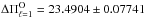 s (Sect. 3.1) and Teff = 90 000 ± 900 K (Hügelmeyer et al. 2006), along with VV 47, with
  s (Sect. 3.2) and Teff = 130 000 ± 13 000 K (Werner & Herwig 2006). The figure shows that the greater the stellar mass, the lower the values of the asymptotic period spacing.
When we linearly interpolate the theoretical values of , the comparison between  and
and  yields a stellar mass of
 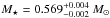 for SDSS J0349−0059. Proceeding similarly for VV 47 (when there were no points to perform the linear interpolation, we extrapolated the theoretical values of ) the comparison between and
  gives a stellar mass of
  (
( ) if VV 47 is after (before) the evolutionary knee. Both values agree excellently well with each other. The errors quoted for VV 47 are admittedly tiny and are unrealistic because of the large uncertainties in the effective temperature. They only represent the internal errors involved in the procedure.
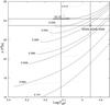 |
Fig. 8 Dipole (ℓ = 1) asymptotic period spacing, |

As in our previous works, we emphasize that deriving the stellar mass using the asymptotic period spacing may not be entirely reliable in pulsating PG 1159 stars that exhibit short and intermediate periods (see Althaus et al. 2008). This is because the asymptotic predictions are strictly valid in the limit of very high radial order (very long periods) and for chemically homogeneous stellar models, while PG 1159 stars are assumed to be chemically stratified and characterized by strong chemical gradients built up during the progenitor star’s life.
In the next section we employ another method to infer the stellar mass of PG 1159 stars. Even though this method is computationally expensive because requires detailed pulsation computations, it has the advantage of being more realistic.
4.2. Second method: comparing the observed period spacing ( ) with the average of the computed period spacings (
 )
)
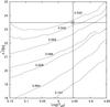 |
Fig. 9 Dipole average of the computed period spacings, |
The average of the computed period spacings is assessed as  , where the “forward” period spacing is defined as ΔΠk = Πk + 1 − Πk (k being the radial order) and n is the number of theoretical periods within the range of periods observed in the target star. For SDSS J0349−0059, Πk ∈ [ 300,970 ] s and for VV 47, Πk ∈ [ 160,5700 ] s.
In Fig. 9 we show the run of the average of the computed period spacings (ℓ = 1) for SDSS J0349−0059 in terms of the effective temperature for our PG 1159 evolutionary sequences (without the sequence of M⋆ = 0.515 M⊙), along with the observed period spacing for SDSS J0349−0059. The figure shows that the greater the stellar mass, the lower the average values of the computed period spacings. After a linear interpolation of the theoretical values of  , the comparison between and
  yields a stellar mass of M⋆ = 0.535 ± 0.004 M⊙. This value is lower than derived through the asymptotic period spacing, which shows that the asymptotic approach overestimates the stellar mass of PG 1159 stars for stars pulsating with short and intermediate periods, which is precisely the situation of SDSS J0349−0059. The value obtained by this approach is more reliable because the method is valid for short, intermediate, and long periods as long as the average of the computed period spacing is evaluated at the correct range of periods.
To investigate the possibility that the period spacings at ~16.5 and ~11.6 s found in Sect. 3.1 might be associated with quadrupole (ℓ = 2) modes, we repeated these calculations, but this time for ℓ = 2. If  s, the stellar mass should then be much lower than M⋆ = 0.530 M⊙. On the other hand, if
  s, then the stellar mass should be ~0.741M⊙. In conclusion, both possible period spacing would lead to values of the stellar mass that are too different from those given by the other determinations, in particular, the value derived using the spectroscopic parameters (M⋆ = 0.543 ± 0.004 M⊙, Sect. 2). This analysis, along with the arguments presented in Sect. 3.1 based on the relation between the asymptotic period spacings for ℓ = 1 and ℓ = 2, allows discarding these values as probable period spacings associated with ℓ = 2.
We depict in Fig. 10 the run of the average of the computed period spacings (ℓ = 1) in terms of the effective temperature for our PG 1159 evolutionary sequences for VV 47 (including M⋆ = 0.515 M⊙). The observed period spacing for VV 47 is also shown. By adopting the effective temperature of VV 47 as given by spectroscopy, we found a stellar mass of  if the star is before the knee, and
  if the star is after the knee. These values are very close to those derived from the asymptotic period spacing, as is expected because this star pulsates with very long periods, almost in the asymptotic regime.
5. Constraints from the individual observed periods
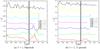 |
Fig. 11 Inverse of the quality function of the period fit considering ℓ = 1 versus Teff for SDSS J0349−0059, adopting the sets of 10 (left panel) and 11 (right panel) periods (see text for details). The vertical gray strip depicts the spectroscopic Teff of SDSS J0349−0059 and its uncertainties. For clarity, the curves have been arbitrarily shifted upward (with a step of 0.05 in the left panel and 0.1 in the right panel) except for the lowest curve. The asteroseismological model has M⋆ = 0.542 M⊙. |
In this procedure we search for a pulsation model that best matches the individual pulsation periods of a given star under study. The goodness of the match between the theoretical pulsation periods ( ) and the observed individual periods (
 ) is measured by means of a merit function defined as
 ![Mathematical equation: \begin{equation} \label{chi} \chi^2(M_{\star}, T_{\rm eff})= \frac{1}{m} \sum_{i=1}^{m} \min\left[\left(\Pi_i^{\rm O}- \Pi_k^{\rm T}\right)^2\right], \end{equation}](/articles/aa/full_html/2016/05/aa27996-15/aa27996-15-eq211.png) (2)where m is the number of observed periods. The PG 1159 model that shows the lowest value of χ2, if one exists, is adopted as the best-fit model. This approach has been used in GW Vir stars by Córsico et al. (2007a,b, 2008, 2009a) and Kepler et al. (2014). We assess the function χ2 = χ2(M⋆,Teff) for stellar masses of 0.515, 0.530, 0.542, 0.565, 0.589, 0.609, 0.664, and 0.741 M⊙. For the effective temperature we employ a much finer grid (ΔTeff = 10−30 K), which is given by the time step adopted by our evolutionary calculations.
(2)where m is the number of observed periods. The PG 1159 model that shows the lowest value of χ2, if one exists, is adopted as the best-fit model. This approach has been used in GW Vir stars by Córsico et al. (2007a,b, 2008, 2009a) and Kepler et al. (2014). We assess the function χ2 = χ2(M⋆,Teff) for stellar masses of 0.515, 0.530, 0.542, 0.565, 0.589, 0.609, 0.664, and 0.741 M⊙. For the effective temperature we employ a much finer grid (ΔTeff = 10−30 K), which is given by the time step adopted by our evolutionary calculations.
5.1. Searching for the best-fit model for SDSS J0349−0059
We started our analysis by assuming that all of the observed periods correspond to ℓ = 1 modes and considered two different sets of observed periods to compute the quality function given by Eq. (2). We began by considering the set of periods listed in boldface in Tables 1 and 2, but with a difference: the values numerically too close each other were averaged; it is not expected that they correspond to independent modes. This resulted in a total of ten periods to be included in the period fit. Figure 11a shows the quantity (χ2)-1 in terms of the effective temperature for different stellar masses, taking into account this set of periods. We also included the effective temperature of SDSS J0349−0059 and its uncertainty (vertical lines). As mentioned before, the goodness of the match between the theoretical and observed periods is measured by the value of χ2: the better the period match, the lower the value of χ2, in our case, the greater the value of (χ2)-1. For this case, there is a strong maximum of (χ2)-1 for a model with M⋆ = 0.609 M⊙ and Teff ~ 69 000 K, as can be seen in Fig. 11a. But although it represents a very good agreement between the observed and the theoretical periods, the effective temperature of this possible solution is unacceptably far from the Teff of SDSS J0349−0059. Another less pronounced maximum corresponds to models with M⋆ = 0.542 M⊙ and Teff ~ 72 000 K, M⋆ = 0.565 M⊙ and Teff ~ 80 000 K, M⋆ = 0.530 M⊙ and Teff ~ 77 000 K, and finally, M⋆ = 0.542 M⊙ and Teff ~ 91 000 K. This last model is closer to the effective temperature of SDSS J0349−0059, and we therefore adopted this model as the asteroseismological model.
Next, we carried out a period fit considering a set of periods from Tables 1 and 2, but adding a set of six periods that were previously discarded (i.e., 353.79 s, 412.27 s, 482.58 s, 504.18 s, 516.72 s, and 517.84 s). Once again, the values numerically too close each other were averaged, which finally resulted in a set of 11 periods. The outcome of the period fit in this case is displayed in Fig. 11b. Compared with the results from the first period fit (Fig. 11a), the function (χ2)-1 is characterized by a smoother behavior, although the peak at ~91 000 K still remains. As a result, there are no new solutions.
For the adopted asteroseismological model, we can compare the observed and the theoretical periods (ℓ = 1, m = 0) by computing the absolute period differences | δΠ | = | ΠO−ΠT |. The results are shown in Table 4. Column 5 of Table 4 shows the value of the linear nonadiabatic growth rate (η), defined as η (≡ −ℑ(σ)/ℜ(σ), where ℜ(σ) and ℑ(σ) are the real and the imaginary part, respectively, of the complex eigenfrequency σ, computed with the nonadiabatic version of the LP-PUL pulsation code (Córsico et al. 2006). A value of η> 0 (η< 0) implies an unstable (stable) mode (see Col. 6 of Table 4). Most periods of the asteroseismological model for SDSS J0349−0059 are associated with unstable modes. Our nonadiabatic computations fail to predict the unstable modes with periods at ~909 s and ~963 s observed in the star. The main features of the asteroseismological model for SDSS J0349−0059 are summarized in Table 5.
Observed periods compared with theoretical periods corresponding to the asteroseismological model for SDSS J0349−0059, with M⋆ = 0.542 M⊙ and Teff = 91 255 K (ℓ = 1, m = 0).
Main characteristics of the asteroseismological model for SDSS J0349−0059.
Next, we considered the possibility that the periods exhibited by the star are a mix of ℓ = 1,2g-modes. The results are shown in Fig. 12 for the same set of observed periods as were considered in Fig. 11a. In the first case (Fig. 12a), new possible solutions arise that can in principle represent good period fits, but the peaks lie well beyond the range allowed by the uncertainties in the effective temperature of SDSS J0349−0059. For the second set of 11 periods displayed in Fig. 12b, new possible solutions closer to the effective temperature of SDSS J0349−0059 arise, but there is no definite asteroseismological model. Altogether, since the period fits considering a mix of ℓ = 1 and ℓ = 2 modes do not show a clear solution, the results point out that the modes of SDSS J0349−0059 are probably only associated with ℓ = 1.
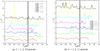 |
Fig. 12 Same as Fig. 11, but comparing the observed periods with theoretical ℓ = 1 and ℓ = 2 periods. In both panels the curves have been arbitrarily shifted upward (with a step of 1) except for the lower curve. |
5.2. Searching for the best-fit model for VV 47
For VV 47, we proceeded analogously to SDSS J0349−0059, but distinguishing the cases before the knee and after the knee. We carried the procedure out by considering three different sets of observed periods. The results of the search for the best-fit model for this star before the knee, considering only ℓ = 1 theoretical modes, can be appreciated in Fig. 13. Figure 13a corresponds to the complete set of periods and shows no unambiguous asteroseismological model in the range of Teff allowed by the spectroscopy. For the reduced list of 11 periods (see Sect. 3.2), Fig. 13b shows many local maxima as well for different masses at several values of the effective temperature, with roughly the same amplitude of (χ2)-1. However, it is possible to find some models that may constitute good period fits considering the range of the effective temperature, and, at the same time, discarding the models with too high masses (compared to the other mass determinations for this star). These models correspond to a mass of M⋆ = 0.530 M⊙ at Teff ~ 124 500 K and Teff ~ 131 000 K. In the third case (Fig. 13c) the set corresponds to the eight longest periods from the complete list (from 1181 s to 5682 s), and once again, there is no unambiguous solution in the range allowed by the effective temperature. However, it is also possible in this case to discard models, therefore we tentatively chose a solution for M⋆ = 0.530 M⊙ and Teff close to the effective temperature of VV 47. The strong peak in the three cases we considered corresponds to the model with M⋆ = 0.542 M⊙. However, in this case, the Teff is too low to be considered a solution, taking into account the constraint given by the spectroscopy. Reversing the argument, the period fit is so good that this might be an indication of a very inaccurate determination of the effective temperature from spectroscopy for this star.
When we analyzed the case after the knee, we found the results shown in Fig. 14. Again, there are multiple local maxima in the three cases. When we considered only the solutions that lie inside the range given for the uncertainty of the effective temperature and discarded those possible solutions associated with too high masses (as compared with the other mass determinations for this star), we adopted a possible solution for the mass M⋆ = 0.515 M⊙ at Teff ~ 126 300 K, but this solution does not touch the value of the effective temperature of the star and is therefore not completely reliable.
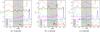 |
Fig. 13 Inverse of the quality function of the period fit considering ℓ = 1 modes only in terms of the effective temperature for VV 47 assuming that the star is before the knee for three different sets of periods (see text for details). The vertical wide strip in gray depicts the spectroscopic Teff and its uncertainties. The curves have been arbitrarily shifted upward (with a step of 0.02 for the left panel, 0.025 for the middle panel, and 0.04 for the right panel), except for the lowest curves. It is possible to adopt a model with M⋆ = 0.530 M⊙. |
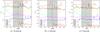 |
Fig. 14 Same as Fig. 13, but for VV 47 evolving after the knee. The curves have been arbitrarily shifted upward (with a step of 0.02 for the left panel and 0.04 for the middle and right panel), except for the lower curve. |
Next, we also considered the possibility that the periods exhibited by VV 47 are a mix of ℓ = 1 and ℓ = 2 modes. In Fig. 15 we show the results corresponding to the three set of periods considered for VV 47 before the knee. For the complete set of periods (Fig. 15a) there are several possible equivalent solutions within the constraint given by the spectroscopy that are consistent with the other determinations of the stellar mass. In the second case (Fig. 15b) we can appreciate a possible solution with M⋆ = 0.530 M⊙, which is close to the Teff of VV 47. In the third case (Fig. 15c), this possible solution is even more evident, and we therefore conclude that a model with M⋆ = 0.530 M⊙ and Teff ~ 130 000 K may be considered a seismological solution, although it is not unique.
Finally, we considered the case in which VV 47 is after the knee, and the results are shown in Fig. 16. In the first case, corresponding to the complete set of observed periods (Fig. 16a), the curves behave very smoothly, and there is no evident solution. The second case, on the other hand, is displayed in Fig. 16b. Here, there may be possible solutions within the uncertainty range for Teff that can be adopted as representative models of VV 47 for M⋆ = 0.515 M⊙ at Teff ~ 120 000 K. In the third case, which is shown in Fig. 16c, the situation is quite similar to the second case, and we may adopt the same solution. As for ℓ = 1, this sequence does not reach the value of the effective temperature given for this star, so this solution may not be accurate.
We close this section by emphasizing that, all in all, for VV 47 we were unable to find a clear and unambiguous seismological solution on the basis of our set of PG 1159 evolutionary models. This prevents us from adopting a representative asteroseismological model for this star (as we did for SDSS J0349−0059), and thus from inferring its internal structure.
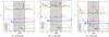 |
Fig. 15 Inverse of the quality function of the period fit considering a mix of ℓ = 1,2 modes in terms of the effective temperature for VV 47 before the knee for three different sets of periods (see text for details). The vertical gray strip depicts the spectroscopic Teff and its uncertainties. The curves have been arbitrarily shifted upward (with a step of 1) except for the lowest curve. It is possible to adopt a model with M⋆ = 0.530 M⊙. |
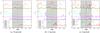 |
Fig. 16 Same as Fig. 15, but for VV 47 after the knee. |
6. Rotation of SDSS J0349−0059
As noted by Woudt et al. (2012), there is a probable frequency triplet in the 2007 data set at 2372.6μHz, 2387.2μHz, and 2401.4 μHz (421.48 s, 418.90 s, and 416.42 s, respectively). This makes a first-order analysis of the rotational splitting feasible from which to estimate the rotation period, Prot = 1/Ω, of SDSS J0349−0059.
In absence of rotation, each eigenfrequency of a nonradially pulsating star is (2ℓ + 1)-fold degenerate. Under the assumption of slow rotation, which is the case for most white dwarfs and pre-white dwarfs (Fontaine & Brassard 2008; Charpinet et al. 2009; Althaus et al. 2010), the perturbation theory can be applied to the first order. The frequency degeneration is lifted, and each component of the resulting multiplet can be calculated as σk,ℓ,m(Ω) = σk,ℓ(Ω = 0) + δσk,ℓ,m (Cowling & Newing 1949). If rotation is rigid (Ω = constant), the first-order corrections to the frequency can be expressed as δσk,ℓ,m = −mΩ(1 − Ck,ℓ), where m = 0, ± 1,..., ± ℓ, and Ckℓ are coefficients that depend on the details of the stellar structure and the eigenfunctions and can be obtained in the non-rotating case. When an asteroseismological model is found for the star under study, these coefficients are available (i.e., they result from the pulsation calculations), and this is our case. For SDSS J0349−0059, the asteroseismological model is characterized by Teff = 91 255 K and M⋆ = 0.542 M⊙ (Table 5). If we associate the periods of SDSS J0349−0059 at 416.42 s and 421.48 s with the components of a rotational triplet with m = + 1 and m = −1, respectively, and assume the period 418.90 s as the central component (m = 0) (see Table 1), then Δσ = σ(m = + 1) − σ(m = −1) = 28.8 μHz is the frequency spacing between the extreme components of the triplet. Thus, δσ = Δσ/ 2 = 14.4 μHz. The corresponding value for the coefficient Ck,ℓ is 0.4936, corresponding to the theoretical period closest to the observed period with m = 0 of the asteroseismological model for SDSS J0349−0059. Then, Ω = 28.4360 μHz, leading to a rotation period of Prot = 1/Ω = 0.407 d.
7. Summary and conclusions
We here presented a detailed asteroseismological study of the pulsating PG 1159 stars SDSS J0349−0059 and VV 47, aimed at determining the internal structure and evolutionary stage of these pulsating stars. Our analysis was based on the fully evolutionary PG 1159 models of Althaus et al. (2005), Miller Bertolami & Althaus (2006), and Córsico et al. (2006). The observational data employed for this study were based on the observed periods reported in Woudt et al. (2012) for SDSS J0349−0059 and González Pérez et al. (2006) for VV 47. Employing the spectroscopic data from Hügelmeyer et al. (2006) for SDSS J0349−0059 and Werner & Herwig (2006) for VV 47, we inferred a value for the spectroscopic mass of both stars. The results are M⋆ = 0.543 M⊙ for SDSS J0349−0059 and M⋆ = 0.529 M⊙ for VV 47 (see Fig. 1).
Stellar masses for all pulsating PG 1159 stars that were studied in detail.
Next, we determined the observed period spacing for both stars, employing three different and independent tests. We found  s for SDSS J0349−0059 and
  s for VV 47 (see Sect. 3). Then, making use of the strong dependence of the period spacing of pulsating PG 1159 stars on the stellar mass, we derived the mass for the two stars. First, this was achieved by comparing the observed period spacing with the asymptotic period spacing of our models (which is an inexpensive approach, since it does not involve pulsation computations). We obtained
  for SDSS J0349−0059. For VV 47, we derived
  assuming the star is before the knee, and
  for VV 47 assuming it is after the knee (see Sect. 4.1). A second estimate of M⋆, based on the comparison of the observed period spacings with the average of the computed period spacings (an approach that requires detailed period computations), gives M⋆ = 0.535 ± 0.004 M⊙ for SDSS J0349−0059, and
  (before the knee) and
  (after the knee) for VV 47 (see Sect. 4.2). A third determination was achieved by carrying out period-to-period fits, consisting of searching for models that best reproduce the individual observed periods of each star. The period fits were made on a grid of PG 1159 models with a fine resolution in stellar mass and a much finer grid in effective temperature and considering g-modes with ℓ = 1 and ℓ = 2. For SDSS J0349−0059 we were able to find an asteroseismological model with M⋆ = 0.542 M⊙ and Teff = 91 255 K (for ℓ = 1g-modes) based on the constraint given by the spectroscopy (see Sect. 5.1). The simultaneous search for a period fit for modes ℓ = 1 and ℓ = 2 did not result in an asteroseismological solution, thus indicating that the periods exhibited by this star are associated only with ℓ = 1 modes. We found no clear and unambiguous solution for VV 47 (see Sect. 5.2), which unfortunately prevents us from presenting a representative aseroseismological model for this star and from extracting seismic information of its internal structure. Finally, after we adopted the model with M⋆ = 0.542 M⊙ for SDSS J0349–0059 as the asteroseismological model, we were able to determine the rotation period by employing the observed triplet of frequencies associated with the period 418.90 s (m = 0) (see Sect. 6). We found a rotation period of Prot = 1/Ω = 0.407 d.
In Table 6 we show a compilation of the mass determinations carried out for the most frequently studied pulsating PG 1159 stars that were analyzed on the basis of our set of fully evolutionary models. For VV 47 the values quoted for the mass were obtained by averaging the two estimates we derived here considering that the star evolves before and after the evolutionary knee.
In summary, we were able to find an excellent agreement between our estimates for the stellar mass of both SDSS J0349−0059 and VV 47, which shows the great internal consistency of our analysis. We were able to find an asteroseismological model for SDSS J0349−0059, which implies that we have additional information about this star, such as the stellar radius, luminosity, and gravity (see Table 5). On the other hand, as expected, the determination of the rotation period agrees well with the estimates by Woudt et al. (2012) of Prot = 1/Ω = 0.40 ± 0.01d, and it is also in line with the values determined for other white dwarf and pre-white dwarf stars (see Fontaine & Brassard 2008, Table 4). This result reinforces the assumption that pre-white dwarf stars are slow rotators. It would be valuable to repeat these calculations using an independent set of evolutionary tracks of PG 1159 stars to add reliability to our results. This is beyond the scope of this paper.
Our results are a further step in a series of studies made by our group with the aim to study the internal structure and evolution status of pulsating PG 1159-type stars through the tools of asteroseismology. Our results for the pulsating PG 1159 stars SDSS J0349−0059 and VV 47 show the power of this approach once again, in particular for determining the stellar mass with an unprecedented precision.
For historical reasons, some authors designate planetary nebula nuclei variable (PNNV) to GW Vir stars that are still embedded in a nebula, and DOV to GW Vir stars without planetary nebula (Winget & Kepler 2008), a misnomer because no white dwarf of spectral type DO has ever been found to pulsate.
According to the nomenclature widely accepted in the literature, we use the term “spectroscopic mass”, although the term “evolutionary mass” might be more appropriate, because its derivation involves the employment of evolutionary tracks.
La Plata Stellar Evolution and Pulsation Research Group (http://fcaglp.fcaglp.unlp.edu.ar/evolgroup/)
Acknowledgments
We wish to thank our anonymous referee for the constructive comments and suggestions that greatly improved the original version of the paper. Part of this work was supported by AGENCIA through the Programa de Modernización Tecnológica BID 1728/OC-AR, and by the PIP 112-200801-00940 grant from CONICET. This research made use of NASA Astrophysics Data System.
References
- Althaus, L. G., Serenelli, A. M., Panei, J. A., et al. 2005, A&A, 435, 631 [NASA ADS] [CrossRef] [EDP Sciences] [Google Scholar]
- Althaus, L. G., Córsico, A. H., Kepler, S. O., & Miller Bertolami, M. M. 2008, A&A, 478, 175 [NASA ADS] [CrossRef] [EDP Sciences] [Google Scholar]
- Althaus, L. G., Córsico, A. H., Isern, J., & García-Berro, E. 2010, A&ARv, 18, 471 [NASA ADS] [CrossRef] [Google Scholar]
- Bond, H. E., Kawaler, S. D., Ciardullo, R., et al. 1996, AJ, 112, 2699 [NASA ADS] [CrossRef] [Google Scholar]
- Charpinet, S., Fontaine, G., & Brassard, P. 2009, Nature, 461, 501 [NASA ADS] [CrossRef] [PubMed] [Google Scholar]
- Ciardullo, R., & Bond, H. E. 1996, AJ, 111, 2332 [NASA ADS] [CrossRef] [Google Scholar]
- Córsico, A. H., & Althaus, L. G. 2006, A&A, 454, 863 [NASA ADS] [CrossRef] [EDP Sciences] [Google Scholar]
- Córsico, A. H., Althaus, L. G., & Miller Bertolami, M. M. 2006, A&A, 458, 259 [NASA ADS] [CrossRef] [EDP Sciences] [Google Scholar]
- Córsico, A. H., Althaus, L. G., Miller Bertolami, M. M., & Werner, K. 2007a, A&A, 461, 1095 [NASA ADS] [CrossRef] [EDP Sciences] [Google Scholar]
- Córsico, A. H., Miller Bertolami, M. M., Althaus, L. G., Vauclair, G., & Werner, K. 2007b, A&A, 475, 619 [NASA ADS] [CrossRef] [EDP Sciences] [Google Scholar]
- Córsico, A. H., Althaus, L. G., Kepler, S. O., Costa, J. E. S., & Miller Bertolami, M. M. 2008, A&A, 478, 869 [NASA ADS] [CrossRef] [EDP Sciences] [Google Scholar]
- Córsico, A. H., Althaus, L. G., Miller Bertolami, M. M., & García-Berro, E. 2009a, A&A, 499, 257 [NASA ADS] [CrossRef] [EDP Sciences] [Google Scholar]
- Córsico, A. H., Althaus, L. G., Miller Bertolami, M. M., González Pérez, J. M., & Kepler, S. O. 2009b, ApJ, 701, 1008 [NASA ADS] [CrossRef] [Google Scholar]
- Costa, J. E. S., & Kepler, S. O. 2008, A&A, 489, 1225 [NASA ADS] [CrossRef] [EDP Sciences] [Google Scholar]
- Costa, J. E. S., Kepler, S. O., Winget, D. E., et al. 2008, A&A, 477, 627 [NASA ADS] [CrossRef] [EDP Sciences] [Google Scholar]
- Cowling, T. G., & Newing, R. A. 1949, ApJ, 109, 149 [Google Scholar]
- Fontaine, G., & Brassard, P. 2008, PASP, 120, 1043 [NASA ADS] [CrossRef] [Google Scholar]
- Fu, J.-N., Vauclair, G., Solheim, J.-E., et al. 2007, A&A, 467, 237 [NASA ADS] [CrossRef] [EDP Sciences] [Google Scholar]
- González Pérez, J. M., Solheim, J.-E., & Kamben, R. 2006, A&A, 454, 527 [NASA ADS] [CrossRef] [EDP Sciences] [Google Scholar]
- Handler, G., Pikall, H., O’Donoghue, D., et al. 1997, MNRAS, 286, 303 [NASA ADS] [CrossRef] [Google Scholar]
- Herwig, F., Blöcker, T., Langer, N., & Driebe, T. 1999, A&A, 349, L5 [NASA ADS] [Google Scholar]
- Hügelmeyer, S. D., Dreizler, S., Homeier, D., et al. 2006, A&A, 454, 617 [NASA ADS] [CrossRef] [EDP Sciences] [Google Scholar]
- Iben, Jr., I., Kaler, J. B., Truran, J. W., & Renzini, A. 1983, ApJ, 264, 605 [NASA ADS] [CrossRef] [Google Scholar]
- Kawaler, S. D. 1986, Ph.D. Thesis, Texas Univ., Austin [Google Scholar]
- Kawaler, S. D. 1987, in IAU Colloq. 95: Second Conference on Faint Blue Stars, eds. A. G. D. Philip, D. S. Hayes, & J. W. Liebert, 297 [Google Scholar]
- Kawaler, S. D. 1988, in Advances in Helio- and Asteroseismology, eds. J. Christensen-Dalsgaard, & S. Frandsen, IAU Symp., 123, 329 [Google Scholar]
- Kawaler, S. D. 1990, in Confrontation Between Stellar Pulsation and Evolution, eds. C. Cacciari, & G. Clementini, ASP Conf. Ser., 11, 494 [Google Scholar]
- Kawaler, S. D., & Bradley, P. A. 1994, ApJ, 427, 415 [NASA ADS] [CrossRef] [Google Scholar]
- Kawaler, S. D., Potter, E. M., Vucković, M., et al. 2004, A&A, 428, 969 [NASA ADS] [CrossRef] [EDP Sciences] [Google Scholar]
- Kepler, S. O., Fraga, L., Winget, D. E., et al. 2014, MNRAS, 442, 2278 [NASA ADS] [CrossRef] [Google Scholar]
- Lawlor, T. M., & MacDonald, J. 2003, ApJ, 583, 913 [NASA ADS] [CrossRef] [Google Scholar]
- Liebert, J., Fleming, T. A., Green, R. F., & Grauer, A. D. 1988, PASP, 100, 187 [NASA ADS] [CrossRef] [Google Scholar]
- Miller Bertolami, M. M., & Althaus, L. G. 2006, A&A, 454, 845 [NASA ADS] [CrossRef] [EDP Sciences] [Google Scholar]
- Miller Bertolami, M. M., & Althaus, L. G. 2007a, A&A, 470, 675 [NASA ADS] [CrossRef] [EDP Sciences] [Google Scholar]
- Miller Bertolami, M. M., & Althaus, L. G. 2007b, MNRAS, 380, 763 [NASA ADS] [CrossRef] [Google Scholar]
- O’Donoghue, D. 1994, MNRAS, 270, 222 [NASA ADS] [CrossRef] [Google Scholar]
- Quirion, P.-O., Fontaine, G., & Brassard, P. 2004, ApJ, 610, 436 [NASA ADS] [CrossRef] [Google Scholar]
- Quirion, P.-O., Fontaine, G., & Brassard, P. 2005, A&A, 441, 231 [NASA ADS] [CrossRef] [EDP Sciences] [Google Scholar]
- Quirion, P.-O., Fontaine, G., & Brassard, P. 2007, ApJS, 171, 219 [NASA ADS] [CrossRef] [Google Scholar]
- Quirion, P.-O., Fontaine, G., & Brassard, P. 2009, J. Phys. Conf. Ser., 172, 012077 [NASA ADS] [CrossRef] [Google Scholar]
- Quirion, P.-O., Fontaine, G., & Brassard, P. 2012, ApJ, 755, 128 [NASA ADS] [CrossRef] [Google Scholar]
- Reed, M. D., Kawaler, S. D., & O’Brien, M. S. 2000, ApJ, 545, 429 [NASA ADS] [CrossRef] [Google Scholar]
- Sion, E. M. 1986, PASP, 98, 821 [NASA ADS] [CrossRef] [Google Scholar]
- Tassoul, M. 1980, ApJS, 43, 469 [NASA ADS] [CrossRef] [Google Scholar]
- Vauclair, G., Moskalik, P., Pfeiffer, B., et al. 2002, A&A, 381, 122 [NASA ADS] [CrossRef] [EDP Sciences] [Google Scholar]
- Werner, K., & Herwig, F. 2006, PASP, 118, 183 [NASA ADS] [CrossRef] [Google Scholar]
- Werner, K., & Rauch, T. 2015, A&A, 584, A19 [NASA ADS] [CrossRef] [EDP Sciences] [Google Scholar]
- Werner, K., Rauch, T., & Kepler, S. O. 2014, A&A, 564, A53 [NASA ADS] [CrossRef] [EDP Sciences] [Google Scholar]
- Wesemael, F., Green, R. F., & Liebert, J. 1985, ApJS, 58, 379 [Google Scholar]
- Winget, D. E., & Kepler, S. O. 2008, ARA&A, 46, 157 [NASA ADS] [CrossRef] [EDP Sciences] [Google Scholar]
- Woudt, P. A., Warner, B., & Zietsman, E. 2012, MNRAS, 426, 2137 [NASA ADS] [CrossRef] [Google Scholar]
All Tables
List of the 13 independent frequencies in the 2007 January data of SDSS J0349−0059 from Woudt et al. (2012).
List of the ten independent frequencies in the 2009 December data of SDSS J0349−0059 from Woudt et al. (2012).
Most important peaks in the VV 47 power spectra according to González Pérez et al. (2006).
Observed periods compared with theoretical periods corresponding to the asteroseismological model for SDSS J0349−0059, with M⋆ = 0.542 M⊙ and Teff = 91 255 K (ℓ = 1, m = 0).
All Figures
|
Fig. 1 PG 1159 (VLTP) evolutionary tracks of Miller Bertolami & Althaus (2006; from right to left: M⋆ = 0.515, 0.530, 0.542, 0.565, 0.589, 0.609, 0.664, 0.741 M⊙) in the log Teff − log g diagram (thin dotted curves). The location of all known PG 1159 stars (variable, non-variable, and objects with no variability data) is shown, including SDSS J0349−0059 and VV 47 with their uncertainties. The uncertainty values for SDSS J0349−0059 are very low in the adopted scale and are not visible in the plot. The hot blue edges (blue curves) and the low-gravity red edges (upper red curves) of the theoretical GW Vir instability strip for ℓ = 1 (dashed) and ℓ = 2 (dotted) modes according to Córsico et al. (2006) are also depicted. The high-gravity red edge that is due to the competition of residual stellar winds against the gravitational settling of C and O (Quirion et al. 2012) is also included (lower red solid curve). |
| In the text | |
|
Fig. 2 I-V (upper panel), K-S (middle panel), and F-T significance (bottom panel) tests applied to the period spectrum of SDSS J0349−0059 to search for a constant period spacing. The periods used here are those indicated in Table 1 and 2. |
| In the text | |
|
Fig. 3 Same as Fig. 2, but for the 15 selected periods of SDSS J0349−0059 emphasized with boldface in Tables 1 and 2. |
| In the text | |
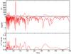 |
Fig. 4 Same as Fig. 2 but for 6 of the discarded periods of SDSS J0349−0059. |
| In the text | |
|
Fig. 5 I-V (upper panel), K-S (middle panel), and F-T (bottom panel) significance tests applied to the period spectrum of VV 47 to search for a constant period spacing. The periods used here are those provided by Table 3, where we considered a single period at 132.05 s instead of the pair of periods at 131.6 s and 132.5 s. No unambiguous signal of a constant period spacing is evident. |
| In the text | |
|
Fig. 6 Same as Fig. 5, but discarding the periods at 132.05 s, 153.5 s, 240.4 s, 280.1 s, and 3521 s of VV 47 from the analysis (see text for details). |
| In the text | |
|
Fig. 7 Same as Fig. 5, but discarding the periods at 132.05 s, 153.5 s, 240.4 s, 280.1 s, 3521 s, and 4310 s of VV 47 from the analysis (see text for details). |
| In the text | |
|
Fig. 8 Dipole (ℓ = 1) asymptotic period spacing, |
| In the text | |
|
Fig. 9 Dipole average of the computed period spacings, |
| In the text | |
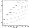 |
Fig. 10 Same as Fig. 9, but for VV 47. |
| In the text | |
|
Fig. 11 Inverse of the quality function of the period fit considering ℓ = 1 versus Teff for SDSS J0349−0059, adopting the sets of 10 (left panel) and 11 (right panel) periods (see text for details). The vertical gray strip depicts the spectroscopic Teff of SDSS J0349−0059 and its uncertainties. For clarity, the curves have been arbitrarily shifted upward (with a step of 0.05 in the left panel and 0.1 in the right panel) except for the lowest curve. The asteroseismological model has M⋆ = 0.542 M⊙. |
| In the text | |
|
Fig. 12 Same as Fig. 11, but comparing the observed periods with theoretical ℓ = 1 and ℓ = 2 periods. In both panels the curves have been arbitrarily shifted upward (with a step of 1) except for the lower curve. |
| In the text | |
|
Fig. 13 Inverse of the quality function of the period fit considering ℓ = 1 modes only in terms of the effective temperature for VV 47 assuming that the star is before the knee for three different sets of periods (see text for details). The vertical wide strip in gray depicts the spectroscopic Teff and its uncertainties. The curves have been arbitrarily shifted upward (with a step of 0.02 for the left panel, 0.025 for the middle panel, and 0.04 for the right panel), except for the lowest curves. It is possible to adopt a model with M⋆ = 0.530 M⊙. |
| In the text | |
|
Fig. 14 Same as Fig. 13, but for VV 47 evolving after the knee. The curves have been arbitrarily shifted upward (with a step of 0.02 for the left panel and 0.04 for the middle and right panel), except for the lower curve. |
| In the text | |
|
Fig. 15 Inverse of the quality function of the period fit considering a mix of ℓ = 1,2 modes in terms of the effective temperature for VV 47 before the knee for three different sets of periods (see text for details). The vertical gray strip depicts the spectroscopic Teff and its uncertainties. The curves have been arbitrarily shifted upward (with a step of 1) except for the lowest curve. It is possible to adopt a model with M⋆ = 0.530 M⊙. |
| In the text | |
|
Fig. 16 Same as Fig. 15, but for VV 47 after the knee. |
| In the text | |
Current usage metrics show cumulative count of Article Views (full-text article views including HTML views, PDF and ePub downloads, according to the available data) and Abstracts Views on Vision4Press platform.
Data correspond to usage on the plateform after 2015. The current usage metrics is available 48-96 hours after online publication and is updated daily on week days.
Initial download of the metrics may take a while.