© ESO, 2016

1. Introduction

A significant part of stars are located in double or multiple stellar systems. However, reviews of pulsating stars bound in binaries (e.g. Szatmáry 1990; Zhou 2010) clearly show the lack of stellar pairs with an RR Lyrae component. The number of currently confirmed binaries comprising an RR Lyrae type pulsator can be counted on one hand.

The binarity of an object can be revealed in many different ways. For example, detection of eclipses, periodic radial velocity (RV) changes, or regular astrometric shifts in a visual binary can serve as a direct proof of binarity. A companion of a periodic variable star can also be detected indirectly through changes in timings of light extrema, the so-called light time effect (hereafter LiTE). RR Lyrae stars are generally located at larger distance from Earth, hence astrometric detection of binarity is highly unlikely. Since the spectra of RR Lyrae stars are influenced by pulsations, discovering the binary nature of stars through changes in the position of spectral lines is also difficult (e.g. Fernley & Barnes 1997; Solano et al. 1997). Thus the most promising methods are detection of eclipses and LiTE.

In the Large Magellanic Cloud (LMC) three candidates for RR Lyraes in eclipsing binaries were detected (Soszyński et al. 2003). However, these objects were identified as optical blends consisting of two objects, RR Lyrae star and eclipsing system (Soszyński et al. 2003; Prša et al. 2008). A very interesting object was identified by Soszyński et al. (2011) and subsequently studied by Pietrzyński et al. (2012) and Smolec et al. (2013). This peculiar eclipsing system with an orbital period of 15.24 d contains a component that mimics an RR Lyrae pulsator. The detailed study showed that this object, OGLE-BLG-RRLYR-02792, has a very low mass of only 0.26 M_{⊙ ,} which is too low for classical RR Lyrae stars. Other physical characteristics also indicate that this binary component is a very special object as a result of an evolution in a close binary followed by a life similar to a classical RR Lyrae star. Pietrzyński et al. (2012) included the object in a new class of pulsating stars called binary evolution pulsators (BEP). OGLE-LMC-RRLYR-03541 is another candidate for RR Lyr in eclipsing binary (Soszyński et al. 2009). Nonetheless, the similarity in the shape of the light curve and the short orbital period of 16.229 d might mean that it belongs to the class of BEP (Hajdu, priv. comm.). In addition, it is not yet excluded that it could be actually a blend of two close stars.

Szatmáry (1990) published a list of various types of pulsating stars bound in binary systems that were visually identified on the basis of the LiTE in their O–C diagrams. However, detailed information and references are missing. The catalogue of various binary systems with pulsating components from Zhou (2010, version December 2014) contains in the RR Lyrae class TU UMa, OGLE-BLG-RRLYR-02792, and several tens of candidates without any closer information. Therefore, including some of these objects as binary systems (in both catalogues) is at least doubtful.

Several examples of RR Lyrae stars in binaries were very recently identified through the analysis of their O–C diagrams. Li & Qian (2014) found that FN Lyr and V894 Cyg are probably in pairs with brown dwarves. Hajdu et al. (2015) found 20 additional candidates among OGLE bulge RRab variables. Liška et al. (2015) presented an analysis of 11 new binary candidates located in the Galactic field. Nevertheless, all these candidates need to be confirmed spectroscopically or using another independent method.

In this paper, we present a new analysis of the LiTE in TU UMa (23-yr long cycle, detected by Szeidl et al. 1986) that is based on a much wider sample of O–C than was used for the LiTE in TU UMa before (Wade et al. 1999). Highly accurate photometric observations that cover two thirds of the proposed orbital period, are newly available. In Sect. 2 we briefly discuss the history of observation of TU UMa with an emphasis on its binary nature. In Sect. 3 we summarise the characteristics of our data sample. Except for data from various sources, we used the original measurements gathered in 2013–2014. We apply our LiTE procedure (described in Sect. 4 and Appendix A) and model the TU UMa data in Sect. 5. Other proofs for binarity are discussed in Sect. 6, and all results are summarised in Sect. 7.

2. History of TU UMa observations

TU Ursae Majoris = AN 1.1929 = BD+30 2162 = HIP 56088 (α = 11^h29^m48$\mathit{.}{}^{\mathrm{s}}$49, δ = +30°04′02.̋4, J2000.0) is a pulsating RR Lyrae star of Bailey ab type. According to the Variable Star Index¹ (Watson et al. 2006), its brightness in V band varies in the range of 9.26–10.24 mag (spectral type A8–F8) with a period of about 0.558 d. No signs of the Blažko effect have been reported for TU UMa up to now.

The variability of TU UMa was discovered by Guthnick & Prager (1929) on Babelsberg plates. Many authors thereafter studied the star using photoelectric photometry and spectroscopy. A detailed description of the history of TU UMa research was performed by Szeidl et al. (1986). Only the most important information about the LiTE is briefly mentioned below, since about 180 articles with the keyword TU UMa are currently retrievable at the NASA ADS portal.

Payne-Gaposchkin (1939) was the first who noted cyclic variations in maxima timings and proposed a 12 400-day (34-yr) long cycle. Important results were obtained by Szeidl et al. (1986), who mentioned a secular period decrease that causes the parabolic trend in the O–C diagram, and a probable 23-yr (8400 d) variation that is possibly caused by the binarity of the star. Saha & White (1990a) detected systematic shifts in RVs that indicate binarity, but they used very few RV measurements. They modelled the LiTE for the first time and determined orbital period of 7374.5 d (20.19 yr). Their analysis showed that the proposed stellar pair has an extremely eccentric orbit with e = 0.970. They considered only a constant pulsation period in their model. The effect of neglecting the secular changes of e, a sini, and M₂ sin³i was tested by Wade et al. (1992).

The LiTE with secular variation in the pulsation period was firstly solved by Kiss et al. (1995), who determined more accurate orbital elements and derived an orbital period of 8800 d (24.1 yr). Wade et al. (1999) collected all available maxima timings and also RVs and successfully verified results from Saha & White (1990a). They obtained five different groups of models of the LiTE with respect to different subsets of maxima timings (all maxima without visual values, only photoelectric and CCD values, etc.). They derived orbital periods in the range from 20.26 yr to 24.13 yr depending on the particular data set and the number of fitting parameters (with or without parabolic trend). Subsequently, they used nine derived sets of orbital elements to reconstruct the orbital RV curve of the pulsating component and to compare it with shifts in observed RVs. Since then, TU UMa has not been studied with regard to its LiTE for about 15 yr. However, improvements of quadratic ephemeris were performed by Arellano Ferro et al. (2013), for instance. Many high-accurate maxima timings (mainly CCD measurements) were published during this 15-yr interval. The currently available data exceed five proposed orbital cycles.

3. Data sources

3.1. GEOS RR Lyrae database

Since the GEOS RR Lyrae database² (Groupe Européen d’Observations Stellaires, Boninsegna et al. 2002; Le Borgne et al. 2007) is the most extended archive of times of RR Lyrae star maxima, we used this as the main data source for our analysis. The version of the database of November 2014 contains corrected values for three maxima timings from Kiss et al. (1995) that originally contained incorrect heliocentric corrections (Wade et al. 1999).

We discarded all visually determined maxima timings because they were inaccurate and omitted two photographic maxima from Robinson & Shapley (1940) and Payne-Gaposchkin (1954), which were replaced by our maxima from the DASCH project (see Sect. 3.3). We used also the latest maxima timings from Hübscher (2014), Hübscher & Lehmann (2015) that were not included in the version of the GEOS list we used.

We paid special attention to maxima timings based on data from sky surveys such as Hipparcos (ESA 1997) or ROTSE = NSVS (Woźniak et al. 2004) for the GEOS values³. These timings were acquired with a special method because in most cases they were determined statistically based on the combination of many points that are often spread out over a few years. O–C values determined from such data sets very often did not follow the general trend of O–C dependence⁴. They were therefore omitted. However, we re-analysed the original data of these surveys (Sect. 3.3). All used maxima timings are available at the CDS portal.

3.2. Our observations

As an extension of the GEOS data we also used ten new maxima timings gathered by J. Liška in 19 nights between December 2013 and June 2014. CCD photometric measurements were performed using two telescopes – three nights with a 24-inch Newtonian telescope (vby Strömgren filters) at Masaryk University Observatory in Brno, and 16 nights with a small 1-inch refractor (green filter with similar throughput as the Johnson V filter, Liška & Lišková 2014) at a private observatory in Brno. For the small-aperture telescope, five frames with exposure times of 30 s each were combined to a single image to achieve a better signal-to-noise ratio. The time resolution of such a combined frame is about 170 s. The comparison star BD+30 2165 was the same for both instruments, but the control stars were BD+30 2164 (for the 24-inch telescope) and HD 99593 (for the 1-inch telescope). Maxima timings were determined via polynomial fitting⁵ or the template fitting described in Sect. 3.3. Monitoring with the small telescope resulted in the well-covered phase light curve shown in Fig. 1. Except for maxima timings determination, the observations were also important for detecting possible eclipse (Sect. 6.2). Our measurements are available at the CDS portal.

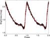Fig. 1 Differential magnitudes of TU UMa obtained with the 1-inch telescope folded with the pulsation period (black dots) plotted together with the model of V-band observations from Liakos & Niarchos (2011a).

3.3. Other sources

We used high-cadence measurements from the SuperWASP project (Pollacco et al. 2006; Butters et al. 2010) and Pi of the Sky project (e.g. Burd et al. 2004; Siudek et al. 2011) to determine maximum timings from the individual well-covered nights.

In addition, to extend the O–C dataset as far as possible, we also analysed data from other large sky surveys (Hipparcos, NSVS) and from the project DASCH (photometry from scanned Harvard plates, e.g. Grindlay et al. 2009). For these very sparse but very extended data, maxima timings were estimated using template fitting. The same process was applied to the data from the other sources.

Firstly, we chose the dataset with the best-quality data and with the best phase-coverage. Since the data from all surveys were of insufficient quality to construct the template light curve (e.g. in Hipparcos and NSVS data the phase around maximum brightness was not observed), V-band measurements from Liakos & Niarchos (2011a) were used. We then modelled the shape of the light curve m(t) in Matlab with a non-linear least-squares method (hereafter LSM) with an n-order harmonic polynomial 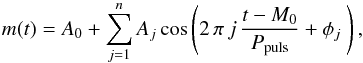$\mathit{m}\mathrm{\left(}\mathit{t}\mathrm{\right)}\mathrm{=}{\mathit{A}}_{\mathrm{0}}\mathrm{+}\sum _{\mathit{j}\mathrm{=}\mathrm{1}}^{\mathit{n}}{\mathit{A}}_{\mathit{j}}\cos \left(\mathrm{2}\hspace{0.17em}\mathit{\pi }\hspace{0.17em}\mathit{j}\hspace{0.17em}\frac{\mathit{t}\mathrm{-}{\mathit{M}}_{\mathrm{0}}}{{\mathit{P}}_{\mathrm{puls}}}\mathrm{+}{\mathit{\phi }}_{\mathit{j}}\right)\mathit{,}$(1)where A₀ is the zeroth level of brightness in mag, A_j are amplitudes of the components in mag, t is the time of observation in Heliocentric Julian Date (HJD), M₀ is the zero epoch of maximal brightness in HJD, P_puls is the pulsation period in days, and φ_j represents the phase shifts in radians. After some experiments, we found that a polynomial with n = 15 is sufficient for a good template model.

Nevertheless, using one template curve for various surveys brings some particularities. Firstly, each dataset has its own magnitude zero level, and the model has to be scaled because different surveys use different filters. Therefore we used the whole light curves for our fit. Individual amplitudes A_j and phase shifts φ_j known from the template curve remained fixed, but the total amplitude was rescaled using the ratio of total amplitudes for the analysed and template datasets. The factor was typically close to 1. In addition, pulsation period and zero epoch had to be slightly refined for each dataset. Subsequently, outliers were iteratively removed.

Individual observational instruments have different spectral sensitivities, therefore it was necessary to verify the usability of the same V-band template for different datasets. We used photometric measurements in UBVRI filters from Liakos & Niarchos (2011a) and compared all curves. The main difference is in amplitude, which is highly dependent on the mean wavelength (the amplitude decreases from 1.3 mag in U to 0.6 mag in I). When the amplitudes are normalised, the differences between shapes of U, B, V, and R curves are almost negligible (comparable with the noise level). The same applies for the times of maxima. Only I-band light changes differ, apparently. Surveys typically observed in broad band filters and mean wavelengths are not known, or the values were only roughly estimated. We can fortunately estimate them using comparison between amplitudes of survey data and UBVRI-amplitudes. We found that effective wavelengths for all surveys lie between the wavelengths of the B and R filters; this means that our approach (V-band template) is applicable.

The good consistence of our template and the observed curves was controlled visually (see Fig. 2). For SuperWASP data, which were obtained using six different CCD cameras, a very careful selection of the best nights compared to the template was performed to avoid significant trends that are present in the data.

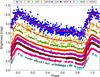Fig. 2 Light curves of TU UMa from different datasets: DA – DASCH A, DB – DASCH B, HIPP – Hipparcos, LIAKOS – Liakos & Niarchos (2011a, V, OUR – this paper (1-inch, green-filter), WASP – SuperWASP (CCD 144), PI – Pi of the Sky, NSVS – NSVS, MODEL – used template curves (DASCH templates are described in Sect. 3.4). Light curves are vertically shifted to better display the light variability.

When the data were sparse without well-defined maxima, it was necessary to divide the whole dataset into smaller subsamples containing typically about 30 points, with a time span from several days to hundreds of days. The data in these subsamples were then compared with the refined template light curve, and the time of maximum was determined. With this subsampling we were of course only able to estimate the mean time of maximum for the time interval of particular subset. However, in comparison with the total time span of the O–C values, which cover several decades, this method is fully appropriate. The numbers of all used maxima timings from particular surveys are listed in Table 1.

In addition, we determined five maxima times from the data that were omitted or only poorly determined from the analysis in Boenigk (1958), Liakos & Niarchos (2011a,b), Liu & Janes (1989), and Preston et al. (1961).

The uncertainty of each time of maximum determined by the template fitting method is influenced mainly by the choice of the used model (selection of polynomial degree), the time determined for the template maximum, and by the quality of the fitted datasets. The first two components were estimated statistically from the template light curve, and their combination was set to 0.0008 d. The influence of the third source of uncertainties was individually estimated for each light curve directly from the LSM.

3.4. Photographic measurements – DASCH maxima timings

Photographic measurements that were obtained with exposure times of an hour and longer are special cases. Light curves resulting from these observations differ from real curves in amplitude and also in time of minima and maxima (for example the models of B-band measurements of TU UMa from Liakos & Niarchos 2011a, in Fig. 3). We performed a detailed analysis of this problem and will publish the results elsewhere. Therefore we discuss only the most important findings. The extrema timings and amplitude change almost linearly with the duration of the exposure time. Maxima are delayed, minima occurred sooner, and the amplitude is lower than for shorter exposures.

Fig. 3 Change of the light curve shape caused by long exposure time. The model of the real light curve based on B-band observations from Liakos & Niarchos (2011a; red line) is plotted together with models of observed curves with exposures of 63 min (black crosses) and 200 min (blue dots).

The photographic plates that were digitalised in the DASCH project have various integration times, mostly from 1 to 200 min (Fig. 4), therefore it is very difficult to correctly analyse the data (different models of the observing curve have to be used). We solved this problem by selecting the measurements with similar exposures (they can be approximated with the same template curve; the time difference is no more than 0.0005 d).

At first, we selected the measurements according to the exposure – group A (58–68 min, older measurements) and group B (30–40 min, newer measurements). Then we calculated template curves for the mean exposures 63 min and 35 min (deformed by the exposure) based on measurements of Liakos & Niarchos (2011a). These two templates were used for the DASCH A and B dataset.

Our tests showed that for ~ 60 min exposure, for instance, the maximum brightness based on exposure-deformed light curve is delayed of about +0.004 d in comparison with real changes. This difference will be apparent, for example, in maxima timings determined using polynomial fitting. Therefore, this shift has to be included in the final maxima times. When the template fitting method is applied with an improved time-corrected model (template from the deformed curve), the exposure-length discrepancy is fully reduced to zero.

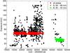Fig. 4 Exposure times of the photographic plates of TU UMa in the DASCH project. The data were divided into two groups according to their integration times – group A with 58–68 min (red crosses) and B with 30–40 min (green stars).

4. Modelling the LiTE

4.1. Light time effect

The LiTE was suggested at the end of the ninteenth century in the Algol system by Chandler (1888), while the first detailed theoretical analysis of the problem was performed by Woltjer (1922). Irwin (1952a) solved important equations for a part of the direct solution of the LiTE and described a graphical way to determine the orbital elements.

Currently, the LiTE is usually solved very accurately by applying equations of motion in a two-body system (the equations from Irwin 1952a included a direct solution of Kepler’s equation) or using numerical calculations of a perturbed orbit in a multiple system. Nevertheless, the inverse part of the calculations, in which the best solution is determined (minimisation), still remains a problem to be discussed – various authors use various methods, for example, damped differential corrections (Pribulla et al. 2000), the LSM (Panchatsaram 1981), the simplex (Levenberg-Marquart) method (Wade et al. 1999; Lee et al. 2010), or a combination of LSM and simplex method (Zasche 2008). For example, the simplex method has several versions that differ in the setting of the initial parameters, sorting conditions, or in the size of corrections. Thus, obtaining the same results, that is, repeat the process, is very difficult, even impossible. To avoid this ambiguity, the inverse part of our code was constructed on the basis of the non-linear LSM described in (e.g., Mikulášek & Zejda 2013) applied to modelling the LiTE (for details see Sect. 4.2 and Appendix A). This way has previously been applied to analyse the LiTE in the AR Aur system (Mikulášek et al. 2011; Chrastina 2013) and is similar to the one used by Van Hamme & Wilson (2007) and Wilson & Van Hamme (2014).

4.2. Fitting procedure

The code that we used is written in Matlab. It consists of several modules: loading measurements and setting initial input parameters, direct solution of the LiTE including an optional parabolic trend, inverse minimisation method, and, finally, selecting the best solution and calculating uncertainties of individual parameters through bootstrap resampling (Sect. 4.3).

A prediction of maxima timings T_cal calculated according to the relation 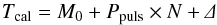${\mathit{T}}_{\mathrm{cal}}\mathrm{=}{\mathit{M}}_{\mathrm{0}}\mathrm{+}{\mathit{P}}_{\mathrm{puls}}\mathrm{\times }\mathit{N}\mathrm{+}\mathit{\Delta }$(2)contains linear ephemeris, as well as correction Δ for the LiTE. The parameter M₀ is the zero epoch of pulsations in HJD, P_puls is the pulsation period in days, and N is the number of pulsation cycle from M₀.

The correction Δ for the LiTE includes calculating the orbit of a pulsating star around the centre of mass of a binary in relative units and can be expressed by the equation adopted from Irwin (1952a)$\mathit{\Delta }\mathrm{=}\mathit{A}\hspace{0.17em}\left[\mathrm{(}\mathrm{1}\mathrm{-}{\mathit{e}}^{\mathrm{2}}\mathrm{)}\hspace{0.17em}\frac{\sin \mathrm{(}\mathit{\nu }\mathrm{+}\mathit{\omega }\mathrm{)}}{\mathrm{1}\mathrm{+}\mathit{e}\hspace{0.17em}\cos \mathit{\nu }}\mathrm{+}\mathit{e}\hspace{0.17em}\sin \mathit{\omega }\right]\mathit{,}$(3)where e is the numerical eccentricity, ω is the argument of periastron (usually in degrees), A ≐ a₁ sini/ 173.145 is the projection of the semi-major axis of primary (pulsating) component a₁ in light days⁶ according to the inclination of the orbit i, and ν is the true anomaly. The eccentric anomaly E, which is necessary to determine the true anomaly ν, is solved with Kepler’s equation by iteratively using Newton’s method with a given precision higher than 1 × 10^-9arcsec. Kepler’s equation requires a mean anomaly M, which is determined from the orbital period P_orbit in days and the time of periastron passage T₀ in HJD.

Another more complex model that includes a parabolic trend in O–C (e.g. Zhu et al. 2012), uses the modified Eq. (2) in the form of 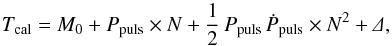${\mathit{T}}_{\mathrm{cal}}\mathrm{=}{\mathit{M}}_{\mathrm{0}}\mathrm{+}{\mathit{P}}_{\mathrm{puls}}\mathrm{\times }\mathit{N}\mathrm{+}\frac{\mathrm{1}}{\mathrm{2}}\hspace{0.17em}{\mathit{P}}_{\mathrm{puls}}\hspace{0.17em}\mathit{Ṗ}\mathrm{puls}\mathrm{\times }{\mathit{N}}^{\mathrm{2}}\mathrm{+}\mathit{\Delta ,}$(4)where P_puls is the instantaneous pulsation period at the moment M₀ and the parameter Ṗ_puls = dP_puls/ dt is the rate of changes in the pulsation period in [d d^-1]. For easy comparison with other RR Lyrae stars, we used prescriptions from Le Borgne et al. (2007). Their parameter a₃ = 1/2 P_pulsṖ_puls is the rate of period changes per one cycle in [d cycle^-1], and the rate of period changes β in [ms d^-1] is β = 6.31152 × 10¹⁰a₃/P_puls or β = 0.07305 × 10¹⁰a₃/P_puls in [d Myr^-1] ⁷. The instantaneous pulsation period at arbitrary epoch N is P_puls(N) = P_puls(M₀) + Ṗ_puls × N.

The first step of the non-linear LSM is linearising the non-linear model function (Eqs. (2) or (4)) by Taylor decomposition of the first order (see Mikulášek et al. 2006; Mikulášek & Gráf 2011) 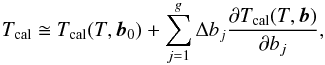${\mathit{T}}_{\mathrm{cal}}\cong {\mathit{T}}_{\mathrm{cal}}\mathrm{\left(}\mathit{T,}{{b}}_{\mathrm{0}}\mathrm{\right)}\mathrm{+}\sum _{\mathit{j}\mathrm{=}\mathrm{1}}^{\mathit{g}}\mathrm{\Delta }{\mathit{b}}_{\mathit{j}}\frac{\mathit{\partial }{\mathit{T}}_{\mathrm{cal}}\mathrm{\left(}\mathit{T,}{b}\mathrm{\right)}}{\mathit{\partial }{\mathit{b}}_{\mathit{j}}}\mathit{,}$(5)where b_j are individual free parameters in vector b. Vector b₀ contains initial estimates of parameters, Δb_j are their corrections, g is the number of free parameters (the length of matrix b).

After linearisation, the problem can be solved in the same way as in the linear LSM, but with several necessary iterations to obtain a precise solution. Our code generates the initial parameters quasi-randomly many times from large intervals with limits that are defined by user. The derivatives are solved analytically. For more details see Appendix A.

The parameter χ²(b_k) or its normalised value ${\mathit{\chi }}_{\mathrm{R}}^{\mathrm{2}}\mathrm{\left(}{{b}}_{\mathit{k}}\mathrm{\right)}\mathrm{=}{\mathit{\chi }}^{\mathrm{2}}\mathrm{\left(}{{b}}_{\mathit{k}}\mathrm{\right)}\mathit{/}\mathrm{(}\mathit{n}\mathrm{-}\mathit{g}\mathrm{)}$, where n is a number of measurements, was used as an indicator of the quality of the k-fit.

Since many maxima timings from the GEOS database are given without errors or are often questionable, we used an alternative approach to determine the weights. The dataset was divided into several groups according to the type of observations (photographic, photoelectric, CCD, DSLR), and weights were assigned to each of the groups with respect to the dispersion of points around the model. The weights were improved iteratively. Groups with fewer than five points (DSLR) were merged with another group with similar data quality to avoid unrealistic weight assignment (CCD+DSLR). During the fitting process, outliers differing by more than 5σ from the model were rejected. All steps of the analysis were supervised visually.

The LiTE fitting process does not allow estimating the masses of the two stars, but only a mass function f(M)$\mathit{f}\mathrm{\left(}M\mathrm{\right)}\mathrm{=}\frac{\mathrm{(}{M}_{\mathrm{2}}\hspace{0.17em}\sin \mathit{i}{\mathrm{)}}^{\mathrm{3}}}{\mathrm{(}{M}_{\mathrm{1}}\mathrm{+}{M}_{\mathrm{2}}{\mathrm{)}}^{\mathrm{2}}}\mathrm{=}\frac{\mathrm{4}\hspace{0.17em}{\mathit{\pi }}^{\mathrm{2}}}{\mathit{G}}\hspace{0.17em}\frac{\mathrm{(}{\mathit{a}}_{\mathrm{1}}\hspace{0.17em}\sin \mathit{i}{\mathrm{)}}^{\mathrm{3}}}{{\mathit{P}}_{\mathrm{orbit}}^{\mathrm{2}}}\mathit{,}$(6)where M₁, M₂ are masses of the components, i is the inclination angle of the orbit, P_orbit is the orbital period, and a₁ is the semi-major axis of the primary component. Based on the studies of Fernley (1993) and Skarka (2014), we adopted as the value for the mass of the RR Lyrae component M₁ = 0.55 M_⊙ and set the inclination angle to i = 90 ° (sini = 1). This allows computing the lowest mass of the second component by solving the cubic equation $M_{\mathrm{2}}^{\mathrm{3}}\mathrm{-}\mathit{f}\mathrm{\left(}M\mathrm{\right)}\hspace{0.17em}{M}_{\mathrm{2}}^{\mathrm{2}}\mathrm{-}\mathrm{2}\hspace{0.17em}\mathit{f}\mathrm{\left(}M\mathrm{\right)}\hspace{0.17em}{M}_{\mathrm{1}}\hspace{0.17em}{M}_{\mathrm{2}}\mathrm{-}\mathit{f}\mathrm{\left(}M\mathrm{\right)}\hspace{0.17em}{M}_{\mathrm{1}}^{\mathrm{2}}\mathrm{=}\mathrm{0.}$(7)We expect that the variation in the O–C diagram of TU UMa can be well described using Eq. (4) and that other possible secular variation of the pulsation period can be neglected (it has a low amplitude or appears to be on a longer timescale).

4.3. Bootstrap-resampling

The (non-linear) LSM itself gives an estimate of the uncertainty of all fitted parameters, but the method is extremely sensitive to data characteristics. A slight change of the dataset by adding one single measurement can cause a significant difference in the new parameters from the previous solution. We therefore decided to use a statistical approach represented by bootstrap-resampling to estimate the errors.

The parameters from the best solution were used as initial values to fit a new dataset, whose points were randomly selected from the original dataset. This procedure was repeated 5000 times. From the scattering of individual parameters of these five thousand solutions, we estimated their uncertainties. The errors in Tables 2 and 3 correspond to 1σ.

4.4. Test object CL Aurigae: an eclipsing binary with probable LiTE and mass transfer

The code was, among others, tested on the well-known detached binary system CL Aur. This eclipsing binary was chosen because it shows the LiTE and a secular period change. In addition, CL Aur was studied in a similar way three times during the past 15 yr (Wolf et al. 1999, 2007; Lee et al. 2010).

The times of minima of CL Aur taken from the O–C gateway database⁸ (Paschke & Brát 2006) were used to construct O–C diagram and to determine parameters through the methods described above⁹. Our best model (Fig. 5) describes the O–C variations very well in the most recent part (precise CCD observations). The old part of the O–C diagram with visual and photographic measurements is highly scattered, but these measurements were also taken into account during the fitting process by assigning them a lower weight (model weights for different observation methods were found in the ratio pg:vis:ccd 1:11.5:403)¹⁰. We conclude that our results are comparable with previous results (Table 2). This example, as well as additional testing, showed that our code works well and is suitable for analysing RR Lyraes with suspected LiTE. The code was successfully used to model the LiTE in V2294 Cyg (Liška 2014).

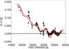Fig. 5 O–C diagram of the testing eclipsing binary CL Aurigae (double star without an RR Lyrae component) with the LiTE and parabolic trend (black circles). The model of changes (red line) is based on our parameters from Table 2.

5. LiTE in TU UMa and analysis of the O–C diagram

Cyclic changes in O–C diagram of TU UMa have been well known for a long time and were analysed in detail by Saha & White (1990a)¹¹, Kiss et al. (1995), and Wade et al. (1999). The parameters determined by these authors are given in Table 3.

Our dataset described in Sect. 3 is much denser and more extended than in previous studies (in contrast to Wade et al. 1999, who used only 83, we used 253 maxima timings). Our O–C values span 113 yr, which is mainly due to measurements recorded on the Harvard plates (provided by the project DASCH) in the first half of the twentieth century. Because the complete dataset is not homogeneous (it has incomparably better coverage over the last two decades with CCD measurements), we analysed LiTE in TU UMa in two ways. Model 1 is based on the whole dataset¹², while model 2 describes only photoelectric, CCD, and DSLR observations¹³. Since TU UMa experiences secular period decrease (in Fig. 6 represented by the parabolic dot-dashed curve) with the rate 1/2 P_pulsṖ_puls of about −2.9 × 10^-11 days per cycle (Wade et al. 1999), we used the complex form of the model (Eq. (4)).

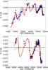Fig. 6 O–C diagram of TU UMa. Black circles and blue stars display the maxima adopted from the GEOS database and new maxima determined in this work. The period decrease manifested by the parabolic trend (dot–dashed line) is obvious. Cyclic changes due to an orbital motion are also clearly visible. Our model of LiTE is represented by the solid red line. The top panel shows model 1 with all available data, while the plot in the bottom panel shows the situation with only photoelectric, CCD, and DSLR observations (model 2).

Logically, model 1, which is based on the whole data set (covering five orbital periods) gives more precise, but slightly different results than model 2, which spans only two of the 23-yr orbital cycles. Nevertheless, high-accurate photoelectric and CCD measurements cover the whole orbital cycle very well (see Fig. 7). Because of the shorter time base, our second model has a lower value of the secular period evolution, for example. This happens at the expense of an increasing eccentricity (0.66 and 0.69 for models 1 and 2, respectively) and change in the argument of periastron (181 and 184°).

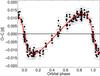Fig. 7 O–C diagram of TU UMa constructed only from photoelectric, CCD, and DSLR measurements after subtracting the parabolic trend and phased with the orbital period based on model 2.

In comparison with orbital elements from previous studies given in Table 3, our results have a higher confidence level that is due to the larger and better dataset. Our values differ mainly in eccentricity and distance between components and in the mass function. All these values were found to be significantly lower than those from Saha & White (1990a), Kiss et al. (1995), or Wade et al. (1999). Values from Saha & White (1990a) differ more because they neglected the period decrease.

The eccentricity is not as extreme as proposed by Saha & White (1990a). Its value is comparable with other systems from Hajdu et al. (2015), Li & Qian (2014).

Based on our results, it seems that TU UMa is very likely a member of a well-detached system with a dwarf component with a minimal mass of only 0.33 M_⊙. Since no signs of the companion are observed in the light of TU UMa, it is probably a late-type main-sequence dwarf star. However, we cannot exclude the possibility that it is a white dwarf or a neutron star, since we do not know the inclination.

Except for the LiTE, which is the most remarkable feature of the O–C diagram, changes represented by the parabolic trend are also apparent. The progression of the dependence suggests secular shortening of the pulsation period of TU UMa, which is almost certainly an evolutionary effect because the mass transfer, which is responsible for period changes in close binaries, can be excluded because of the very wide orbit of TU UMa. In addition, value β = Ṗ_puls ~ −2.2 ms yr^-1 = −0.026 d Myr^-1 can correspond to a blueward evolution of the RR Lyrae component, but Le Borgne et al. (2007), for instance, reported a higher median value β = −0.20 d Myr^-1 for their sample of 21 stars with a significant period decrease.

After subtracting our model 1 from the whole dataset (Fig. 8), several photographic measurements (in the range of between JD 2 425 000 and 2 429 000) are deviate more than other values, with a systematic shift of about 15 min (0.01 d). This might indicate that TU UMa undergoes more complex period changes than the LiTE and parabolic trend alone. Some possible explanations such as cubic trend or an additional LiTE could describe this variation. However, even though the influence of longer exposure of photographic measurements was taken into account, some other instrumental artefact might play a role.

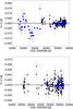Fig. 8 Residual O–C diagram of TU UMa after subtracting the first LiTE model (top panel) and second model – only photoelectric, CCD, and DSLR observations (bottom). Black circles and blue stars display maxima adopted from the GEOS database and new maxima determined in this work. The jump in the general trend of O–C in the range from JD 2 425 000 to 2 429 000 (top panel) might be an indication of a more complex period change.

6. Other proofs for binarity

Since the LiTE is only an indirect manifestation of binarity, it is necessary to prove it in a different way. The analysis of the mean RVs can be considered as the most valuable test. In addition to this method, other possible approaches with which the binarity of TU UMa can be confirmed are discussed in the next sections.

6.1. Radial velocities

The known orbital parameters from the analysis of the LiTE allow us to predict, but also reconstruct, the RV curve from the past. The binarity can then be proved by comparing the model for the orbital RV curve and the spectroscopically determined centre-of-mass RV. This analysis was first performed for TU UMa by Saha & White (1990a) and a few years later by Wade et al. (1999). They noted systematic shifts in the RV determined at different times. Their predictions correlate fairly well with measurements.

We scanned the literature for RV measurements and found nine sources (Table 4). Unfortunately, the last available dataset with RVs was published in 1997. Saha & White (1990a) used only three RV sources, Wade et al. (1999) did not give their values. In addition, both authors ignored the RV measurements from Preston & Paczynski (1964). Other authors have reported slightly different values determined from the same dataset (Table 5, Col. 2) without listing the mean time of observation. Therefore we decided to re-analyse all available RV measurements.

Determining the centre of mass of the RV for a binary with a pulsating star is more complicated than for a binary with non-variable stars (pulsations are often the dominant source of RV changes). Other inconveniences are connected with an RV based on different types of spectral lines (e.g. Balmer or metallic lines). They are formed at different depths, and therefore RV curves from different lines have different shapes, amplitudes, and zero points (shown e.g. by Sanford 1949; Oke et al. 1962). Since available RV measurements are based on various lines, it was necessary to unify them. This was done using the highly accurate normalised template curves from Sesar (2012). Firstly we modelled these template curves with an n-order harmonic polynomial. The observed RV curve for the particular spectral line was then compared with the polynomial image of the template, and the amplitude and the central value of RV curve was simultaneously determined by the LSM for all datasets. Before this step, measurements were time-corrected for binary orbit and period shortening (based on model 1), and several of the datasets were divided into smaller groups to obtain a time resolution of about one year (see Table 5 with the determined mean RVs for given epochs corresponding to the mean value of observation time). We did not find original RV measurements for two studies (Fernley & Barnes 1997; Solano et al. 1997) and therefore adopted their mean RV values and estimated the mean time of observation from the information provided in their papers. Finally, the mean centre of mass of the RV values were compared with the RV model resulting from our LiTE analysis (Fig. 9). The points roughly follow the model RV curve.

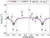Fig. 9 Models of variations in RV caused by orbit of pulsating component around mass-centre of the binary system (red and blue lines) and center-of-mass velocities determined for each dataset of RV measurements using template fitting or adopted from literature. The visually estimated correction −91 km s-1 for systematic velocity mass-centre of the system from Sun (γ-velocity) was applied.

An alternative test for binarity using RV curves can be performed by comparing the observed RV curves (the top panel of Fig. 10) and those in which the orbital RV curve from the model is subtracted (the bottom panel of Fig. 10). In this figure RV measurements are phased according to the pulsation period¹⁴. Apparently, the phased RV curve with corrected velocities is significantly less vertically scattered than without the correction. The residual scatter in the bottom panel results from the different metallic lines that the RVs were based on.

Both tests clearly show that TU UMa is very likely bound in a binary system.

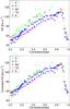Fig. 10 Radial velocity curves from the metallic lines of TU UMa from different publications phased with the pulsation period corrected for the LiTE and secular period changes. Uncorrected observed RVs (top) and corrected values after subtracting the changes in RV caused by orbital motion based on our model 1 (bottom). RV values corrected for binary orbit are evidently less scattered than uncorrected RVs.

6.2. Eclipses

A detection of eclipses in the light curve (in the appropriate phase of the orbit) would be a strong proof for binarity of TU UMa. Several third components of eclipsing binary stars that were known only from the LiTE were confirmed by detecting additional eclipses (e.g. in the Kepler project, Slawson et al. 2011). The probability of catching an eclipse in TU UMa is very low because the expected orbital period of the binary system is very long and radius and luminosity of the secondary component are probably much smaller and lower than for the pulsating star. In addition, the inclination angle of the orbit is unknown. Our two preliminary LiTE models allow us to estimate the time of a possible eclipse, where the RR Lyrae component should transit the secondary one (January – February 2014 or May – June 2014), but the difference between the two predictions is too large. However, we attempted to detect the proposed eclipse.

Observations with the small telescope described in Sect. 3.2 were dedicated for this purpose. Unfortunately, our measurements were insufficient for a reliable decision about eclipses. Weather conditions, limited object visibility and other influences allowed us to observe in only 19 nights, which is hardly sufficient considering the imprecise eclipse prediction. At least we can conclude that no sign of an eclipse with an amplitude higher than 0.07 mag was detected in our data (see Fig. 11).

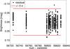Fig. 11 Residuum of the light curve of TU UMa after subtracting the harmonic polynomial model. No signs of an eclipse with an amplitude higher than 0.07 mag was detected in the green band.

7. Summary and conclusions

We presented a new analysis of a probable LiTE in TU UMa. We used published maxima timings from the GEOS database (168 values) and added maxima values from our photometric observations and from the SuperWASP and Pi of the Sky surveys. We applied the template fitting method to determine maxima from these measurements and also from sparse data from the projects Hipparcos, NSVS and DASCH. Altogether, we analysed 253 maxima timing measurements, which is about three times more than were used in the dataset in the last study of TU UMa by Wade et al. (1999). This large and well covered dataset allowed us to determine a quadratic ephemeris of the pulsations and orbital elements of the binary system with much better accuracy than in previous studies (Table 3). All analyses were performed with a new code written in Matlab that uses a bootstrap method to estimate the errors. We calculated two models: model 1, which describes the whole dataset (without visual maxima timings), and model 2, which describes only high-accurate photoelectric, CCD and DSLR maxima. The second model is based on data with a significantly shorter time span than for model 1.

The second model gives a lower value of the period-decrease rate (β = Ṗ_puls ~ −1.4 ms yr^-1), which causes the eccentricity to become higher (e ~ 0.69) than in the first model (β ~ −2.2 ms yr^-1, e ~ 0.66). For comparison, Arellano Ferro et al. (2013) give β = −1.3 ms yr^-1 without fitting the LiTE. Nevertheless, both our models have a lower eccentricity value, semi-major axis of pulsating component a₁ sini (2.9 au or 3.0 au), and semi-amplitude of RV variations of the pulsating star K₁ (5.0 km s^-1 or 5.3 km s^-1) than in previous works. Our values of the orbital period (identically 23.3 yr) and argument of periastron ω (181° or 184°) are comparable with values determined by previous authors. In addition, the lowest mass limit of the secondary component (0.33 M_⊙ or 0.34 M_⊙) was determined with an assumption for the mass of the RR Lyrae component of 0.55 M_⊙.

The binary nature was tested in several ways. Firstly, our models of the orbit gave predictions of possible eclipses. Although the prediction was highly inaccurate and an eclipse is highly unlikely (wide orbit, unknown inclination, and other important parameters) we attempted to detect them, but were unfortunately not successful.

Binarity is expected manifest itself in cyclic changes of the mean RV. We adopted RV measurements from nine independent sources and corrected their values according to our model by subtracting the LiTE and secular changes. When an observed RV curve was phased with the pulsation period, we obtained the typical RV curve for RR Lyrae, which was scattered. The scatter significantly decreased when our model was applied.

We also determined central RV values for each RV dataset using pulsation templates for different spectral lines from Sesar (2012). We compared these values with our model of orbital RV variations based on orbital parameters known from the LiTE. The correlation is evident (Fig. 9).

The two successful proofs are important for confirming the binarity of TU UMa. However, only long-term spectroscopic measurements covering the whole orbital cycle can unambiguously confirm that TU UMa is indeed a member of a binary system.

Acknowledgments

The DASCH project at Harvard is grateful for partial support from NSF grants AST-0407380, AST-0909073, and AST-1313370. This paper makes use of data from the DR1 of the WASP data (Butters et al. 2010) as provided by the WASP consortium, and the computing and storage facilities at the CERIT Scientific Cloud, reg. No. CZ.1.05/3.2.00/08.0144, which is operated by Masaryk University, Czech Republic. This research has made use of NASA’s Astrophysics Data System. Work on the paper has been supported by LH14300. M.S. acknowledges the support of the postdoctoral fellowship programme of the Hungarian Academy of Sciences at the Konkoly Observatory as a host institution. We are very grateful to the anonymous referee, who significantly helped to improve this paper.

References

Appendix A: Application of the non-linear LSM on calculating the LiTE

We assumed a group of n maxima timings given in Heliocentric Julian Date¹⁵ (HJD) determined from observations. Times are inserted in the column vector y with a size n × 1. Each time of an observed maximum T_l has a corresponding uncertainty σ_l. We assumed that the quality of the l-measurement can be quantified by the l-weight using the relation ${\mathit{w}}_{\mathit{l}}\mathrm{=}{\mathit{\sigma }}_{\mathit{l}}^{-2}$, and these weights were inserted in the column vector w. For a correct calculation, the weights were normalised (the average value of weights is $\overline{\mathit{w}}\mathrm{=}\mathrm{1}$) and were inserted in a square matrix W = diag(w).

In the next step, we selected the equation for the model function T_cal(T,b) with unknown parameters in vector b. Changes in the position times of the maxima for a pulsating star that are caused by the LiTE (periodic changes in the O–C diagram) can be expressed by ${\mathit{T}}_{\mathrm{cal}}\mathrm{\left(}\mathit{T,}{b}\mathrm{\right)}\mathrm{=}{\mathit{M}}_{\mathrm{0}}\mathrm{+}{\mathit{P}}_{\mathrm{puls}}\mathrm{\times }\mathit{N}\mathrm{+}\mathit{\Delta ,}$(A.1)where M₀ is the zero epoch of pulsation in HJD, P_puls is the pulsation period in days, N is the number of pulsation cycles from M₀, and parameter Δ is the correction for the LiTE. The integer number of the pulsation cycle (epoch) N is $\mathit{N}\mathrm{=}\mathrm{round}\left(\frac{\mathit{T}\mathrm{-}{\mathit{M}}_{\mathrm{0}}}{{\mathit{P}}_{\mathrm{puls}}}\right)\mathrm{·}$(A.2)An optional more complex model that includes the parabolic trend in the O–C diagram (e.g. Zhu et al. 2012) uses the modified Eq. (A.1) in the form of ${\mathit{T}}_{\mathrm{cal}}\mathrm{\left(}\mathit{T,}{b}\mathrm{\right)}\mathrm{=}{\mathit{M}}_{\mathrm{0}}\mathrm{+}{\mathit{P}}_{\mathrm{puls}}\mathrm{\times }\mathit{N}\mathrm{+}\frac{\mathrm{1}}{\mathrm{2}}\hspace{0.17em}{\mathit{P}}_{\mathrm{puls}}\hspace{0.17em}\mathit{Ṗ}\mathrm{puls}\mathrm{\times }{\mathit{N}}^{\mathrm{2}}\mathrm{+}\mathit{\Delta ,}$(A.3)where P_puls is the instantaneous pulsation period at the moment M₀, and parameter Ṗ_puls = dP_puls/ dt is the rate of changes in the pulsation period.

The correction Δ for the LiTE includes calculating the orbit of the pulsating star around the binary mass centre in relative units and is given by the equation adopted from (Irwin 1952a) $\mathit{\Delta }\mathrm{=}\mathit{A}\hspace{0.17em}\left[\mathrm{(}\mathrm{1}\mathrm{-}{\mathit{e}}^{\mathrm{2}}\mathrm{)}\hspace{0.17em}\frac{\sin \mathrm{(}\mathit{\nu }\mathrm{+}\mathit{\omega }\mathrm{)}}{\mathrm{1}\mathrm{+}\mathit{e}\hspace{0.17em}\cos \mathit{\nu }}\mathrm{+}\mathit{e}\hspace{0.17em}\sin \mathit{\omega }\right]\mathit{,}$(A.4)where e is the numerical eccentricity, ν the true anomaly, ω the argument of periastron in degrees, and A is a constant in light days, which compares the shift in a radial position to the time delay caused by the constant speed of light. 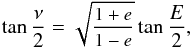The true anomaly ν is calculated from $\tan \frac{\mathit{\nu }}{\mathrm{2}}\mathrm{=}\sqrt{\frac{\mathrm{1}\mathrm{+}\mathit{e}}{\mathrm{1}\mathrm{-}\mathit{e}}}\tan \frac{\mathit{E}}{\mathrm{2}}\mathit{,}$(A.5)and the eccentric anomaly E is iteratively determined in our code by Newton’s method from Kepler’s equation 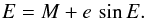$\mathit{E}\mathrm{=}\mathit{M}\mathrm{+}\mathit{e}\hspace{0.17em}\sin \mathit{E}\mathit{.}$(A.6)The mean anomaly M is in the form 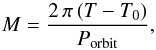$\mathit{M}\mathrm{=}\frac{\mathrm{2}\hspace{0.17em}\mathit{\pi }\hspace{0.17em}\mathrm{(}\mathit{T}\mathrm{-}{\mathit{T}}_{\mathrm{0}}\mathrm{)}}{{\mathit{P}}_{\mathrm{orbit}}}\mathit{,}$(A.7)where the orbital period P_orbit is in days and the time of periastron passage T₀ in HJD.

The constant A is the projection of the semi-major axis of the pulsating component a₁ on the unit light day 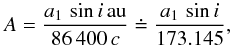$\mathit{A}\mathrm{=}\frac{{\mathit{a}}_{\mathrm{1}}\hspace{0.17em}\sin \mathit{i}\hspace{0.17em}\mathrm{au}}{\mathrm{86}\hspace{0.17em}\mathrm{400}\hspace{0.17em}\mathit{c}}\doteq \frac{{\mathit{a}}_{\mathrm{1}}\hspace{0.17em}\sin \mathit{i}}{\mathrm{173.145}}\mathit{,}$(A.8)where i is the inclination angle of the orbit in degrees, au is length of the astronomical unit in metres, c is the speed of the light in vacuum in m s^-1. The semi-amplitude of LiTE changes in the O–C diagram in days is then ${\mathit{A}}_{\mathrm{LiTE}}\mathrm{=}\mathit{A}\hspace{0.17em}\sqrt{\mathrm{1}\mathrm{-}{\mathit{e}}^{\mathrm{2}}\hspace{0.17em}{\cos }^{\mathrm{2}}\mathit{\omega }}\mathit{.}$(A.9)Subsequently, the observed values of the time of maximum can be compared with those from the model obtained from Eqs. (A.1) and (A.3). Their difference for a given set of parameters is equal to $\mathit{\delta }{\mathit{T}}_{\mathit{l}}\mathrm{=}{\mathit{T}}_{\mathit{l}}\mathrm{-}{\mathit{T}}_{\mathrm{cal}\mathit{,l}}\mathrm{\left(}{\mathit{T}}_{\mathit{l}}\mathit{,}{b}\mathrm{\right)}\mathit{.}$(A.10)The LSM described in detail in (Mikulášek & Zejda 2013) points that the best model has the lowest sum of squares of residuals between observation and model. The modified form of the LSM used the weighted form $\mathit{\delta }{\mathit{T}}_{\mathrm{mod}\mathit{,l}}\mathrm{=}\frac{\mathit{\delta }{\mathit{T}}_{\mathit{l}}}{{\mathit{\sigma }}_{\mathit{l}}}\mathrm{=}\frac{{\mathit{T}}_{\mathit{l}}\mathrm{-}{\mathit{T}}_{\mathrm{cal}\mathit{,l}}\mathrm{\left(}{\mathit{T}}_{\mathit{l}}\mathit{,}{b}\mathrm{\right)}}{{\mathit{\sigma }}_{\mathit{l}}}\mathit{,}$(A.11)and then the sum is $\begin{array}{ccc}{\mathit{\chi }}^{\mathrm{2}}\mathrm{\left(}{b}\mathrm{\right)}\mathrm{=}\sum _{\mathit{l}\mathrm{=}\mathrm{1}}^{\mathit{n}}{\mathit{\delta T}}_{\mathrm{mod}\mathit{,l}}^{\mathrm{2}}& \mathrm{=}& \sum _{\mathit{l}\mathrm{=}\mathrm{1}}^{\mathit{n}}{\left[\frac{{\mathit{T}}_{\mathit{l}}\mathrm{-}{\mathit{T}}_{\mathrm{cal}\mathit{,l}}\mathrm{\left(}{\mathit{T}}_{\mathit{l}}\mathit{,}{b}\mathrm{\right)}}{{\mathit{\sigma }}_{\mathit{l}}}\right]}^{\mathrm{2}}\\ & \mathrm{=}& \sum _{\mathit{l}\mathrm{=}\mathrm{1}}^{\mathit{n}}\mathrm{[}\mathit{\delta }{\mathit{T}}_{\mathit{l}}^{\mathrm{2}}\hspace{0.17em}{\mathit{w}}_{\mathit{l}}\mathrm{]}\mathit{.}\end{array}$(A.12)Its normalised value ${\mathit{\chi }}_{\mathrm{R}}^{\mathrm{2}}\mathrm{\left(}{{b}}_{\mathit{k}}\mathrm{\right)}\mathrm{=}{\mathit{\chi }}^{\mathrm{2}}\mathrm{\left(}{{b}}_{\mathit{k}}\mathrm{\right)}\mathit{/}\mathrm{(}\mathit{n}\mathrm{-}\mathit{g}\mathrm{)}$, where n is the number of measurements and g is the number of free parameters (the length of matrix b), was used as an indicator of the quality of the k-fit.

The first step of the non-linear LSM is linearisation of the non-linear model function (Eqs. (A.1) or (A.3)) by a Taylor decomposition of the first order (see Mikulášek et al. 2006; Mikulášek & Gráf 2011) ${\mathit{T}}_{\mathrm{cal}}\cong {\mathit{T}}_{\mathrm{cal}}\mathrm{\left(}\mathit{T,}{{b}}_{\mathrm{0}}\mathrm{\right)}\mathrm{+}\sum _{\mathit{j}\mathrm{=}\mathrm{1}}^{\mathit{g}}\mathrm{\Delta }{\mathit{b}}_{\mathit{j}}\frac{\mathit{\partial }{\mathit{T}}_{\mathrm{cal}}\mathrm{\left(}\mathit{T,}{{b}}_{\mathrm{0}}\mathrm{\right)}}{\mathit{\partial }{\mathit{b}}_{\mathit{j}}}\mathit{,}$(A.13)where b_j are individual free parameters from the vector b, vector b₀ contains the initial estimates of the parameters, and Δb_j are their corrections in the vector Δb.

Important equations for solving non-linear LSM by matrices are $\hspace{0.17em}\begin{array}{c}\begin{array}{c}\end{array}{U}\mathrm{=}{{X}}^{{T}}\hspace{0.17em}{W}\hspace{0.17em}{\Delta }{y}\mathit{,} {V}\mathrm{=}{{X}}^{{T}}\hspace{0.17em}{W}\hspace{0.17em}{X}\mathit{,}\\ \begin{array}{c}\end{array}{H}\mathrm{=}{{V}}^{-1}\mathrm{=}\mathrm{(}{{X}}^{{T}}\hspace{0.17em}{W}\hspace{0.17em}{X}{\mathrm{)}}^{-1}\mathit{,} {\Delta }{b}\mathrm{=}{H}\hspace{0.17em}{U}\mathit{,}\end{array}$(A.14)

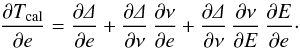
from which the new parameters in vector b₁ can be calculated as b₁ = b₀ + Δb. The difference between observed values and model is Δy = y−T_cal. The matrix with the derivatives has the form $\begin{array}{ccc}{X}\mathrm{=}\left[\frac{\mathit{\partial }{\mathit{T}}_{\mathrm{cal}}}{\mathit{\partial }{\mathit{M}}_{\mathrm{0}}}\mathit{,}\frac{\mathit{\partial }{\mathit{T}}_{\mathrm{cal}}}{\mathit{\partial }{\mathit{P}}_{\mathrm{puls}}}\mathit{,}\frac{\mathit{\partial }{\mathit{T}}_{\mathrm{cal}}}{\mathit{\partial }{\mathit{T}}_{\mathrm{0}}}\mathit{,}\frac{\mathit{\partial }{\mathit{T}}_{\mathrm{cal}}}{\mathit{\partial }{\mathit{P}}_{\mathrm{orbit}}}\mathit{,}\frac{\mathit{\partial }{\mathit{T}}_{\mathrm{cal}}}{\mathit{\partial A}}\mathit{,}\frac{\mathit{\partial }{\mathit{T}}_{\mathrm{cal}}}{\mathit{\partial \omega }}\mathit{,}\frac{\mathit{\partial }{\mathit{T}}_{\mathrm{cal}}}{\mathit{\partial e}}\right]\mathit{,}& & \end{array}$(A.15)where individual derivatives are also presented $\begin{array}{ccc}\frac{\mathit{\partial }{\mathit{T}}_{\mathrm{cal}}}{\mathit{\partial }{\mathit{M}}_{\mathrm{0}}}\mathrm{=}\mathrm{1}\mathit{,} \frac{\mathit{\partial }{\mathit{T}}_{\mathrm{cal}}}{\mathit{\partial }{\mathit{T}}_{\mathrm{0}}}\mathrm{=}\frac{\mathit{\partial \Delta }}{\mathit{\partial \nu }}\hspace{0.17em}\frac{\mathit{\partial \nu }}{\mathit{\partial E}}\hspace{0.17em}\frac{\mathit{\partial E}}{\mathit{\partial M}}\hspace{0.17em}\frac{\mathit{\partial M}}{\mathit{\partial }{\mathit{T}}_{\mathrm{0}}}\mathit{,}& & \end{array}$$\begin{array}{ccc}\frac{\mathit{\partial }{\mathit{T}}_{\mathrm{cal}}}{\mathit{\partial }{\mathit{P}}_{\mathrm{puls}}}\mathrm{=}\mathit{N,} \frac{\mathit{\partial }{\mathit{T}}_{\mathrm{cal}}}{\mathit{\partial }{\mathit{P}}_{\mathrm{orbit}}}\mathrm{=}\frac{\mathit{\partial \Delta }}{\mathit{\partial \nu }}\hspace{0.17em}\frac{\mathit{\partial \nu }}{\mathit{\partial E}}\hspace{0.17em}\frac{\mathit{\partial E}}{\mathit{\partial M}}\hspace{0.17em}\frac{\mathit{\partial M}}{\mathit{\partial }{\mathit{P}}_{\mathrm{orbit}}}\mathit{,}& & \end{array}$$\begin{array}{ccc}\frac{\mathit{\partial }{\mathit{T}}_{\mathrm{cal}}}{\mathit{\partial A}}\mathrm{=}\frac{\mathrm{(}\mathrm{1}\mathrm{-}{\mathit{e}}^{\mathrm{2}}\mathrm{)}\hspace{0.17em}\sin \mathrm{(}\mathit{\nu }\mathrm{+}\mathit{\omega }\mathrm{)}}{\mathrm{1}\mathrm{+}\mathit{e}\hspace{0.17em}\cos \mathit{\nu }}\mathrm{+}\mathit{e}\hspace{0.17em}\sin \mathit{\omega ,}& & \end{array}$$\begin{array}{ccc}\frac{\mathit{\partial }{\mathit{T}}_{\mathrm{cal}}}{\mathit{\partial \omega }}\mathrm{=}\mathit{A}\hspace{0.17em}\left[\frac{\mathrm{(}\mathrm{1}\mathrm{-}{\mathit{e}}^{\mathrm{2}}\mathrm{)}\hspace{0.17em}\cos \mathrm{(}\mathit{\nu }\mathrm{+}\mathit{\omega }\mathrm{)}}{\mathrm{1}\mathrm{+}\mathit{e}\hspace{0.17em}\cos \mathit{\nu }}\mathrm{+}\mathit{e}\hspace{0.17em}\cos \mathit{\omega }\right]\mathit{,}& & \end{array}$$\begin{array}{ccc}\frac{\mathit{\partial }{\mathit{T}}_{\mathrm{cal}}}{\mathit{\partial e}}\mathrm{=}\frac{\mathit{\partial \Delta }}{\mathit{\partial e}}\mathrm{+}\frac{\mathit{\partial \Delta }}{\mathit{\partial \nu }}\hspace{0.17em}\frac{\mathit{\partial \nu }}{\mathit{\partial e}}\mathrm{+}\frac{\mathit{\partial \Delta }}{\mathit{\partial \nu }}\hspace{0.17em}\frac{\mathit{\partial \nu }}{\mathit{\partial E}}\hspace{0.17em}\frac{\mathit{\partial E}}{\mathit{\partial e}}\mathrm{·}& & \end{array}$

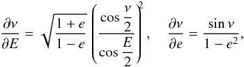
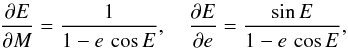
Other necessary derivatives are

$\begin{array}{ccc}\frac{\mathit{\partial \Delta }}{\mathit{\partial \nu }}\mathrm{=}\frac{\mathit{A}\hspace{0.17em}\mathrm{(}\mathrm{1}\mathrm{-}{\mathit{e}}^{\mathrm{2}}\mathrm{)}}{\mathrm{1}\mathrm{+}\mathit{e}\hspace{0.17em}\cos \mathit{\nu }}\hspace{0.17em}\left[\cos \mathrm{(}\mathit{\nu }\mathrm{+}\mathit{\omega }\mathrm{)}\mathrm{+}\frac{\mathit{e}\hspace{0.17em}\sin \mathrm{(}\mathit{\nu }\mathrm{+}\mathit{\omega }\mathrm{)}\hspace{0.17em}\sin \mathit{\nu }}{\mathrm{1}\mathrm{+}\mathit{e}\hspace{0.17em}\cos \mathit{\nu }}\right]\mathit{,}& & \end{array}$$\begin{array}{ccc}\frac{\mathit{\partial \Delta }}{\mathit{\partial e}}\mathrm{=}\mathit{A}\hspace{0.17em}\left\{\sin \mathit{\omega }\mathrm{-}\frac{\sin \mathrm{(}\mathit{\nu }\mathrm{+}\mathit{\omega }\mathrm{)}\hspace{0.17em}\mathrm{[}\mathrm{2}\hspace{0.17em}\mathit{e}\mathrm{+}\mathrm{(}\mathrm{1}\mathrm{+}{\mathit{e}}^{\mathrm{2}}\mathrm{\left)}\hspace{0.17em}\cos \mathit{\nu }\mathrm{\right]}}{\mathrm{(}\mathrm{1}\mathrm{+}\mathit{e}\hspace{0.17em}\cos \mathit{\nu }{\mathrm{)}}^{\mathrm{2}}}\right\}\mathit{,}& & \end{array}$$\begin{array}{ccc}\frac{\mathit{\partial \nu }}{\mathit{\partial E}}\mathrm{=}\sqrt{\frac{\mathrm{1}\mathrm{+}\mathit{e}}{\mathrm{1}\mathrm{-}\mathit{e}}}\hspace{0.17em}{\left(\frac{\cos \frac{\mathit{\nu }}{\mathrm{2}}}{\cos \frac{\mathit{E}}{\mathrm{2}}}\right)}^{\mathrm{2}}\mathit{,} \frac{\mathit{\partial \nu }}{\mathit{\partial e}}\mathrm{=}\frac{\sin \mathit{\nu }}{\mathrm{1}\mathrm{-}{\mathit{e}}^{\mathrm{2}}}\mathit{,}& & \end{array}$$\begin{array}{ccc}\frac{\mathit{\partial E}}{\mathit{\partial M}}\mathrm{=}\frac{\mathrm{1}}{\mathrm{1}\mathrm{-}\mathit{e}\hspace{0.17em}\cos \mathit{E}}\mathit{,} \frac{\mathit{\partial E}}{\mathit{\partial e}}\mathrm{=}\frac{\sin \mathit{E}}{\mathrm{1}\mathrm{-}\mathit{e}\hspace{0.17em}\cos \mathit{E}}\mathit{,}& & \end{array}$$\begin{array}{ccc}\frac{\mathit{\partial M}}{\mathit{\partial }{\mathit{P}}_{\mathrm{orbit}}}\mathrm{=}\frac{\mathrm{-}\mathrm{2}\hspace{0.17em}\mathit{\pi }\hspace{0.17em}\mathrm{(}\mathit{T}\mathrm{-}{\mathit{T}}_{\mathrm{0}}\mathrm{)}}{{\mathit{P}}_{\mathrm{orbit}}^{\mathrm{2}}}\mathit{,} \frac{\mathit{\partial M}}{\mathit{\partial }{\mathit{T}}_{\mathrm{0}}}\mathrm{=}\frac{\mathrm{-}\mathrm{2}\hspace{0.17em}\mathit{\pi }}{{\mathit{P}}_{\mathrm{orbit}}}\mathrm{·}& & \end{array}$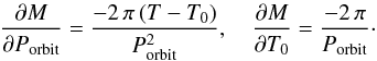Matrix X will be expanded by about one additional member to calculate the parabolic trend according to Eq. (A.3) $\begin{array}{ccc}{X}\mathrm{=}[\frac{\mathit{\partial }{\mathit{T}}_{\mathrm{cal}}}{\mathit{\partial }{\mathit{M}}_{\mathrm{0}}}\mathit{,}\frac{\mathit{\partial }{\mathit{T}}_{\mathrm{cal}}}{\mathit{\partial }{\mathit{P}}_{\mathrm{puls}}}\mathit{,}\frac{\mathit{\partial }{\mathit{T}}_{\mathrm{cal}}}{\mathit{\partial }{\mathit{T}}_{\mathrm{0}}}\mathit{,}\frac{\mathit{\partial }{\mathit{T}}_{\mathrm{cal}}}{\mathit{\partial }{\mathit{P}}_{\mathrm{orbit}}}\mathit{,}\frac{\mathit{\partial }{\mathit{T}}_{\mathrm{cal}}}{\mathit{\partial A}}\mathit{,}& & \\ \frac{\mathit{\partial }{\mathit{T}}_{\mathrm{cal}}}{\mathit{\partial \omega }}\mathit{,}\frac{\mathit{\partial }{\mathit{T}}_{\mathrm{cal}}}{\mathit{\partial e}}\mathit{,}\frac{\mathit{\partial }{\mathit{T}}_{\mathrm{cal}}}{\mathit{\partial }\mathit{Ṗ}\mathrm{puls}}]\mathit{,}& & \end{array}$(A.16)

where two of X members are in the form $\begin{array}{ccc}\frac{\mathit{\partial }{\mathit{T}}_{\mathrm{cal}}}{\mathit{\partial }{\mathit{P}}_{\mathrm{puls}}}\mathrm{=}\mathit{N}\mathrm{+}\frac{\mathrm{1}}{\mathrm{2}}\hspace{0.17em}\mathit{Ṗ}\mathrm{puls}\mathrm{\times }{\mathit{N}}^{\mathrm{2}}\mathit{,} \frac{\mathit{\partial }{\mathit{T}}_{\mathrm{cal}}}{\mathit{\partial }\mathit{Ṗ}\mathrm{puls}}\mathrm{=}\frac{\mathrm{1}}{\mathrm{2}}\hspace{0.17em}{\mathit{P}}_{\mathrm{puls}}\mathrm{\times }{\mathit{N}}^{\mathrm{2}}\mathit{.}& & \end{array}$The determined parameters allow calculating the radial velocity (RV) changes caused by the secondary component (e.g. Irwin 1952b) $\mathit{R}{\mathit{V}}_{\mathrm{1}}\mathrm{=}\mathit{\gamma }\mathrm{+}{\mathit{K}}_{\mathrm{1}}\left[\cos \mathrm{(}\mathit{\nu }\mathrm{+}\mathit{\omega }\mathrm{)}\mathrm{+}\mathit{e}\hspace{0.17em}\cos \mathit{\omega }\right]\mathit{,}$(A.17)where γ is systematic velocity mass-centre of the binary system from the Sun in km s^-1 (γ-velocity) and K₁ is the semi-amplitude of RV changes in km s^-1 given by ${\mathit{K}}_{\mathrm{1}}\mathrm{=}\frac{\mathrm{2}\hspace{0.17em}\mathit{\pi }\hspace{0.17em}{\mathit{a}}_{\mathrm{1}}\hspace{0.17em}\sin \mathit{i}\hspace{0.17em}\mathrm{au}}{\mathrm{8.64}\mathrm{\times }{\mathrm{10}}^{\mathrm{7}}\hspace{0.17em}{\mathit{P}}_{\mathrm{orbit}}\sqrt{\mathrm{(}\mathrm{1}\mathrm{-}{\mathit{e}}^{\mathrm{2}}\mathrm{)}}}\mathit{,}$(A.18)where the projection of the semi-major axis a₁ sini is in au, the constant au in meters, and the orbital period P_orbit in days.

All Tables

All Figures

	Fig. 1 Differential magnitudes of TU UMa obtained with the 1-inch telescope folded with the pulsation period (black dots) plotted together with the model of V-band observations from Liakos & Niarchos (2011a).
In the text

	Fig. 2 Light curves of TU UMa from different datasets: DA – DASCH A, DB – DASCH B, HIPP – Hipparcos, LIAKOS – Liakos & Niarchos (2011a, V, OUR – this paper (1-inch, green-filter), WASP – SuperWASP (CCD 144), PI – Pi of the Sky, NSVS – NSVS, MODEL – used template curves (DASCH templates are described in Sect. 3.4). Light curves are vertically shifted to better display the light variability.
In the text

	Fig. 3 Change of the light curve shape caused by long exposure time. The model of the real light curve based on B-band observations from Liakos & Niarchos (2011a; red line) is plotted together with models of observed curves with exposures of 63 min (black crosses) and 200 min (blue dots).
In the text

	Fig. 4 Exposure times of the photographic plates of TU UMa in the DASCH project. The data were divided into two groups according to their integration times – group A with 58–68 min (red crosses) and B with 30–40 min (green stars).
In the text

	Fig. 5 O–C diagram of the testing eclipsing binary CL Aurigae (double star without an RR Lyrae component) with the LiTE and parabolic trend (black circles). The model of changes (red line) is based on our parameters from Table 2.
In the text

Fig. 6 O–C diagram of TU UMa. Black circles and blue stars display the maxima adopted from the GEOS database and new maxima determined in this work. The period decrease manifested by the parabolic trend (dot–dashed line) is obvious. Cyclic changes due to an orbital motion are also clearly visible. Our model of LiTE is represented by the solid red line. The top panel shows model 1 with all available data, while the plot in the bottom panel shows the situation with only photoelectric, CCD, and DSLR observations (model 2).

In the text

	Fig. 7 O–C diagram of TU UMa constructed only from photoelectric, CCD, and DSLR measurements after subtracting the parabolic trend and phased with the orbital period based on model 2.
In the text

Fig. 8 Residual O–C diagram of TU UMa after subtracting the first LiTE model (top panel) and second model – only photoelectric, CCD, and DSLR observations (bottom). Black circles and blue stars display maxima adopted from the GEOS database and new maxima determined in this work. The jump in the general trend of O–C in the range from JD 2 425 000 to 2 429 000 (top panel) might be an indication of a more complex period change.

In the text

	Fig. 9 Models of variations in RV caused by orbit of pulsating component around mass-centre of the binary system (red and blue lines) and center-of-mass velocities determined for each dataset of RV measurements using template fitting or adopted from literature. The visually estimated correction −91 km s-1 for systematic velocity mass-centre of the system from Sun (γ-velocity) was applied.
In the text

Fig. 10 Radial velocity curves from the metallic lines of TU UMa from different publications phased with the pulsation period corrected for the LiTE and secular period changes. Uncorrected observed RVs (top) and corrected values after subtracting the changes in RV caused by orbital motion based on our model 1 (bottom). RV values corrected for binary orbit are evidently less scattered than uncorrected RVs.

In the text

	Fig. 11 Residuum of the light curve of TU UMa after subtracting the harmonic polynomial model. No signs of an eclipse with an amplitude higher than 0.07 mag was detected in the green band.
In the text

References

- Abt, H. A. 1970, ApJS, 19, 387 [NASA ADS] [CrossRef] [Google Scholar]
- Arellano Ferro, A., Peña, J. H., & Figuera Jaimes, R. 2013, Rev. Mexicana Astron. Astrofis., 49, 53 [NASA ADS] [Google Scholar]
- Barnes, T. G. III., Frueh, M. L., Moffett, T. J., et al. 1988, ApJS, 67, 403 [NASA ADS] [CrossRef] [Google Scholar]
- Boenigk, T. 1958, Acta Astron., 8, 13 [NASA ADS] [Google Scholar]
- Boninsegna, R., Vandenbroere, J.,Le Borgne, J. F., & Geos Team 2002, IAU Colloq. 185: Radial and Nonradial Pulsations as Probes of Stellar Physics, 259, 166 [NASA ADS] [Google Scholar]
- Burd, A., Cwiok, M., Czyrkowski, H., et al. 2004, Astron. Nachr., 325, 674 [NASA ADS] [CrossRef] [Google Scholar]
- Butters, O. W., West, R. G., Anderson, D. R., et al. 2010, A&A, 520, L10 [NASA ADS] [CrossRef] [EDP Sciences] [Google Scholar]
- Chandler, S. C. 1888 AJ, 7, 165 [NASA ADS] [CrossRef] [Google Scholar]
- Chrastina, M. 2013, Ph.D. Thesis, DTPA of Masaryk University, Brno, Czech Republic [Google Scholar]
- ESA 1997, The Hipparcos and Tycho Catalogs, ESA SP–1200 [Google Scholar]
- Fernley, J. 1993, A&A, 268, 591 [NASA ADS] [Google Scholar]
- Fernley, J., & Barnes, T. G. 1997, A&AS, 125, 313 [NASA ADS] [CrossRef] [EDP Sciences] [Google Scholar]
- Grindlay, J., Tang, S., Simcoe, R., et al. 2009, ASP Conf. Ser., 410, 101 [NASA ADS] [Google Scholar]
- Guthnick, P., & Prager, R. 1929, Beob. Zirk., 11, 32 [Google Scholar]
- Hajdu, G., Catelan, M., Jurcsik, J., et al. 2015, MNRAS, 449, L113 [NASA ADS] [CrossRef] [Google Scholar]
- Hemenway, M. K. 1975, AJ, 80, 199 [NASA ADS] [CrossRef] [Google Scholar]
- Hübscher, J. 2014, IBVS, 6118, 1 [NASA ADS] [Google Scholar]
- Hübscher, J., & Lehmann, P. B. 2015, IBVS, 6149, 1 [NASA ADS] [Google Scholar]
- Irwin, J. B. 1952a, ApJ, 116, 211 [NASA ADS] [CrossRef] [Google Scholar]
- Irwin, J. B. 1952b, ApJ, 116, 218 [NASA ADS] [CrossRef] [Google Scholar]
- Kiss, L. L., Szatmary, K., Gal, J., & Kaszas, G. 1995, IBVS, 4205, 1 [Google Scholar]
- Layden, A. C. 1993, Ph.D. Thesis, Yale University, New Haven, USA [Google Scholar]
- Layden, A. C. 1994, AJ, 108, 1016 [NASA ADS] [CrossRef] [Google Scholar]
- Le Borgne, J. F., Paschke, A., Vandenbroere, J., et al. 2007, A&A, 476, 307 [NASA ADS] [CrossRef] [EDP Sciences] [Google Scholar]
- Lee, J. W., Kim, Ch.-H., Kim, D. H., et al. 2010, AJ, 139, 2669 [NASA ADS] [CrossRef] [Google Scholar]
- Li, L.-J., & Qian, S.-B. 2014, MNRAS, 444, 600 [NASA ADS] [CrossRef] [Google Scholar]
- Liakos, A., & Niarchos, P. 2011a, IBVS, 6099, 1 [NASA ADS] [Google Scholar]
- Liakos, A., & Niarchos, P. 2011b, IBVS, 5990, 1 [NASA ADS] [Google Scholar]
- Liška, J. 2014, IBVS, 6119, 1 [NASA ADS] [Google Scholar]
- Liška, J., & Lišková, Z. 2014, IBVS, 6124, 1 [NASA ADS] [Google Scholar]
- Liška, J., Skarka, M., Zejda, M., & Mikulášek, Z. 2015, MNRAS, submitted [arXiv:1504.05246] [Google Scholar]
- Liu, T., & Janes, K. A. 1989, ApJS, 69, 593 [NASA ADS] [CrossRef] [Google Scholar]
- Liu, T., & Janes, K. A. 1990, ApJ, 354, 273 [NASA ADS] [CrossRef] [Google Scholar]
- Maintz, G. 2005, A&A, 442, 381 [NASA ADS] [CrossRef] [EDP Sciences] [Google Scholar]
- Mikulášek, Z., & Gráf, T. 2011, ArXiv e-prints [arXiv:1111.1142] [Google Scholar]
- Mikulášek, Z., & Zejda, M. 2013, in Úvod do studia proměnných hvězd (Brno: Masaryk University) [Google Scholar]
- Mikulášek, Z., Wolf, M., Zejda, M., & Pecharová, P. 2006, Ap&SS, 304, 363 [NASA ADS] [CrossRef] [Google Scholar]
- Mikulášek, Z., Žižňovský, J., Zejda, M., et al. 2011, in Magnetic Stars, Proc. Int. Conf., eds. I. I. Romanyuk, & D. O. Kudryavtsev, 431 [Google Scholar]
- Oke, J. B., Giver, L. P., & Searle, L. 1962, ApJ, 136, 393 [NASA ADS] [CrossRef] [Google Scholar]
- Paschke, A., & Brát, L. 2006, OEJV, 23, 13 [NASA ADS] [Google Scholar]
- Panchatsaram, T. 1981, Ap&SS, 77, 179 [NASA ADS] [CrossRef] [Google Scholar]
- Payne-Gaposchkin, C. 1939, PAPS, 81, 189 [Google Scholar]
- Payne-Gaposchkin, C. 1954, Annals of Harvard College Observatory, 113, 151 [NASA ADS] [Google Scholar]
- Pietrzyński, G., Thompson, I. B., Gieren, W., et al. 2012, Nature, 484, 75 [NASA ADS] [CrossRef] [PubMed] [Google Scholar]
- Pollacco, D. L., Skillen, I., Collier Cameron, A., et al. 2006, PASP, 118, 1407 [NASA ADS] [CrossRef] [Google Scholar]
- Preston, G. W., & Paczynski, B. 1964, ApJ, 140, 181 [NASA ADS] [CrossRef] [Google Scholar]
- Preston, G. W., Spinrad, H., & Varsavsky, C. M. 1961, ApJ, 133, 484 [NASA ADS] [CrossRef] [Google Scholar]
- Pribulla, T., Chochol, D., Tremko, J., et al. 2000, Contributions of the Astronomical Observatory Skalnate Pleso, 30, 117 [Google Scholar]
- Prša, A., Guinan, E. F., Devinney, E. J., & Engle, S. G. 2008, A&A, 489, 1209 [NASA ADS] [CrossRef] [EDP Sciences] [Google Scholar]
- Robinson, L. V., & Shapley, H. 1940, Annals of Harvard College Observatory, 90, 27 [NASA ADS] [Google Scholar]
- Saha, A., & White, R. E. 1990a, PASP, 102, 148 [NASA ADS] [CrossRef] [Google Scholar]
- Saha, A., & White, R. E. 1990b, PASP, 102, 495 [NASA ADS] [CrossRef] [Google Scholar]
- Sanford, R. F. 1949, ApJ, 109, 208 [NASA ADS] [CrossRef] [Google Scholar]
- Sesar, B. 2012, AJ, 144, 114 [NASA ADS] [CrossRef] [Google Scholar]
- Siudek, M., Malek, K., Mankiewicz, L., et al. 2011, Acta Polytechnica, 51, 68 [Google Scholar]
- Skarka, M. 2014, MNRAS, 445, 1584 [NASA ADS] [CrossRef] [Google Scholar]
- Slawson, R. W., Prsa, A., Welsh, W. F., et al. 2011, AJ, 142, 160 [NASA ADS] [CrossRef] [Google Scholar]
- Smolec, R., Pietrzyński, G., Graczyk, D., et al. 2013, MNRAS, 428, 3034 [NASA ADS] [CrossRef] [Google Scholar]
- Solano, E., Garrido, R., Fernley, J., & Barnes, T. G. 1997, A&AS, 125, 321 [NASA ADS] [CrossRef] [EDP Sciences] [Google Scholar]
- Soszyński, I., Udalski, A., Szymanski, M., et al. 2003, Acta Astron., 53, 93 [NASA ADS] [Google Scholar]
- Soszyński, I., Udalski, A., Szymański, M. K., et al. 2009, Acta Astron., 59, 1 [NASA ADS] [Google Scholar]
- Soszyński, I., Dziembowski, W. A., Udalski, A., et al. 2011, Acta Astron., 61, 1 [NASA ADS] [Google Scholar]
- Szatmáry, K. 1990, Journal of the American Association of Variable Star Observers, 19, 52 [Google Scholar]
- Szeidl, B., Olah, K., & Mizser, A. 1986, Commun. Konkoly Observatory Hungary, 89, 57 [Google Scholar]
- Van Hamme, W., & Wilson, R. E. 2007, ApJ, 661, 1129 [Google Scholar]
- Wade, R. A., Saha, A., White, R. E., & Fried, R. 1992, BAAS, 24, 1225 [NASA ADS] [Google Scholar]
- Wade, R. A., Donley, J., Fried, R., et al. 1999, AJ, 118, 2442 [NASA ADS] [CrossRef] [Google Scholar]
- Watson, C. L., Henden, A. A., & Price, A. 2006, Society for Astronomical Sciences Annual Symp., 25, 47 [Google Scholar]
- Wilson, R. E., & Van Hamme, W. 2014, ApJ, 780, 151 [NASA ADS] [CrossRef] [Google Scholar]
- Wolf, M., Šarounová, L., Brož, M., & Horan, R. 1999, IBVS, 4683, 1 [NASA ADS] [Google Scholar]
- Wolf, M., Kotková, L., Brát, L., et al. 2007, IBVS, 5780, 1 [NASA ADS] [Google Scholar]
- Woltjer, Jr., J. 1922, Bull. Astron. Inst. Netherlands, 1, 93 [NASA ADS] [Google Scholar]
- Woźniak, P. R., Vestrand, W. T., Akerlof, C. W., et al. 2004, AJ, 127, 2436 [NASA ADS] [CrossRef] [Google Scholar]
- Zasche, P. 2008, ArXiv e-prints [arXiv:0801.4258] [Google Scholar]
- Zhou, A. -Y. 2010, ArXiv e-prints [arXiv:1002.2729] [Google Scholar]
- Zhu, L.-Y., Zejda, M., Mikulášek, Z., et al. 2012, AJ, 144, 37 [NASA ADS] [CrossRef] [Google Scholar]