| Issue |
A&A
Volume 588, April 2016
|
|
|---|---|---|
| Article Number | L5 | |
| Number of page(s) | 4 | |
| Section | Letters | |
| DOI | https://doi.org/10.1051/0004-6361/201527841 | |
| Published online | 15 March 2016 | |
Origin of the Lyman excess in early-type stars⋆
1 INAF, Osservatorio Astrofisico di Arcetri, Largo E. Fermi 5, 50125 Firenze, Italy
e-mail: This email address is being protected from spambots. You need JavaScript enabled to view it.
2 I. Physikalisches Institut der Universität zu Köln, Zülpicher Strasse 77, 50937 Köln, Germany
3 INAF, Istituto di Astrofisica e Planetologia Spaziale, via Fosso del Cavaliere 100, 00133 Roma, Italy
4 IRAM, Avenida Divina Pastora, 7, Núcleo Central, 18012 Granada, Spain
Received: 26 November 2015
Accepted: 16 February 2016
Abstract
Context. Ionized regions around early-type stars are believed to be well-known objects, but until recently, our knowledge of the relation between the free-free radio emission and the IR emission has been observationally hindered by the limited angular resolution in the far-IR. The advent of Herschel has now made it possible to obtain a more precise comparison between the two regimes, and it has been found that about a third of the young H ii regions emit more Lyman continuum photons than expected, thus presenting a Lyman excess.
Aims. With the present study we wish to distinguish between two scenarios that have been proposed to explain the existence of the Lyman excess: (i) underestimation of the bolometric luminosity, or (ii) additional emission of Lyman-continuum photons from an accretion shock.
Methods. We observed an outflow (SiO) and an infall (HCO+) tracer toward a complete sample of 200 H ii regions, 67 of which present the Lyman excess. Our goal was to search for any systematic difference between sources with Lyman excess and those without.
Results. While the outflow tracer does not reveal any significant difference between the two subsamples of H ii regions, the infall tracer indicates that the Lyman-excess sources are more associated with infall signposts than the other objects.
Conclusions. Our findings indicate that the most plausible explanation for the Lyman excess is that in addition to the Lyman continuum emission from the early-type star, UV photons are emitted from accretion shocks in the stellar neighborhood. This result suggests that high-mass stars and/or stellar clusters containing young massive stars may continue to accrete for a long time, even after the development of a compact H ii region.
Key words: stars: early-type / HII regions / ISM: molecules
Based on observations carried out with the IRAM 30 m Telescope. IRAM is supported by INSU/CNRS (France), MPG (Germany) and IGN (Spain).
© ESO, 2016
1. Introduction
Early-type stars are well-known emitters of copious amounts of ultraviolet photons shortward of 912 Å, which are sufficiently energetic to ionize atomic hydrogen. The neutral gas surrounding such stars during their earliest stages is thus ionized by the Lyman-continuum photons, and an H ii region is created. In the ideal case of an optically thin H ii region around a single OB-type star, it is easy to obtain the stellar Lyman-continuum photon rate (NLy) – as well as other relevant parameters of the star – from the radio continuum flux density emitted by the ionized gas (see, e.g., Schraml & Mezger 1969). In turn, from NLy we can estimate the stellar luminosity (see, e.g., Panagia 1973 and Martins et al. 2005). The latter can be measured by other means from the IR emission of the dusty envelope enshrouding the star and then compared to the value obtained from the Lyman continuum. While the two luminosity estimates should match, in practice the one obtained from the IR emission is often significantly greater than that computed from the radio flux. This discrepancy was discussed by Wood & Churchwell (1989a), and a number of explanations were proposed (opacity of the free-free emission, stellar multiplicity, insufficient angular resolution in the IR). The most important of these was probably the enormous difference in resolving power between IR and radio observations. In fact, the bolometric luminosity (Lbol) estimate was based on the IRAS data, whose instrumental beam in the far-IR is >1′much greater than the typical size of a compact (i.e., young) H ii region (<10′′; see, e.g., Wood & Churchwell 1989a) imaged with a radio interferometer. Consequently, the IRAS fluxes are measured over a solid angle encompassing not only the H ii region, but also other (unrelated) stars, and the value of Lbol is overestimated.
With the advent of the ESA Herschel Space Observatory (Pilbratt et al. 2010), it was possible to dramatically improve on the Lbol estimate and thus achieve a more reliable comparison with the luminosity obtained from the Lyman continuum. In a recent study, Cesaroni et al. (2015; hereafter C2015) have compared NLy to Lbol for the sample of compact and ultracompact H ii regions identified by Purcell et al. (2013) in the CORNISH survey (Hoare et al. 2012). The value of Lbol has been estimated for 200 objects by reconstructing the corresponding spectral energy distributions using the far-IR images of the Herschel/Hi-GAL survey of the Galactic plane (Molinari et al. 2010) and ancillary data from 1 mm to the mid-IR. As discussed by C2015 (see their Sect. 4.1), the surprising result is that about one-third of the H ii regions appear to have NLy greater than expected on the basis of their luminosities (see Fig. 1). After taking a number of possible explanations into account, C2015 (see also Sánchez-Monge et al. 2013) demonstrated that this so-called Lyman excess cannot be easily justified. Basically, two scenarios are possible.
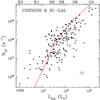 |
Fig. 1 Lyman-continuum photon rate versus the corresponding bolometric luminosity for the 200 CORNISH H ii regions with Herschel/Hi-GAL counterparts studied by C2015. The spectral types indicated at the top are computed under the assumption that Lbol originates from a single ZAMS star. The red solid line denotes the NLy–Lbol relation expected if the H ii regions were powered by single ZAMS stars (see C2015). Note that 67 objects (~34% of the sample) lie above this line. The error bars in the bottom right corner correspond to a 20% calibration uncertainty. |
The first involves the flashlight effect (e.g., Yorke & Bodenheimer 1999), where most stellar photons are leaking along the axis of a bipolar outflow, where the gas density is lower. In this way, a large portion of the photons is emitted away from our line of sight, and the assumption of spherical symmetry adopted in the Lbol calculation leads to an underestimate.
The second scenario assumes that the Lyman excess is due to additional emission of UV photons from the stellar neighborhood. The models adopted to estimate NLy for zero-age main-sequence (ZAMS) stars refer to visible objects, whose properties might be significantly different from those of a very young deeply embedded OB-type star, perhaps still undergoing accretion from the parental cloud. Recent theoretical studies of this type of objects predict significant Lyman-continuum emission from accretion shocks (Smith 2014; Hosokawa & Omukai 2009; Hosokawa, priv. comm.), which may justify an excess of up to two orders of magnitude above the expected value of NLy (see Figs. 15 and 16 of Smith 2014).
If the first scenario is correct, molecular outflows should be more common in Lyman-excess sources than in the rest of the sample. In contrast, the second hypothesis implies that accretion should be preferentially present in the Lyman excess sample. With this in mind, we decided to search for outflow and infall tracers in the whole sample of 200 H ii regions studied by C2015 and thus compare the occurrence of these two phenomena in sources with and without Lyman excess. For this purpose, we observed the HCO+(1–0) and SiO(2–1) lines. The former appears to present redshifted self-absorption when the gas is infalling, while the latter is a well-known tracer of shocked gas in molecular jets and outflows (see, e.g., López-Sepulcre et al. 2010; 2011, and references therein).
2. Observations and data analysis
The observations were performed with the IRAM 30 m telescope on Pico Veleta, using the EMIR receivers (Carter et al. 2012) with the fast Fourier Transform Spectrometer (FTS) at 200 kHz resolution (Klein et al. 2012). By combining two bands of the EMIR receiver, we covered a bandwidth of 16 GHz in dual polarization. While a plethora of potentially useful lines was observed with our setup, in this study we focus on the HCO+(1–0), H13CO+(1–0), and SiO(2–1) rotational transitions. The observations were performed in December 2014 and May and August 2015 using the position-switch mode, where the reference position was chosen from the Herschel/Hi-GAL maps as the closest to the target with minimal continuum emission at 350 μm. In this way, we maximized the likelihood that molecular line emission is also very faint. The on-source integration time per target was 4 min, although for a limited number of faint emitters the integration was repeated twice. We pointed on strong nearby quasars every ~1.5 h. Pointing corrections were stable, with errors below 3". Typical system temperatures ranged from 105 K to 200 K at 3 mm and from 120 K to 400 K at 2 mm. The instrumental half-power beam width was ~27′′.
The data reduction and analysis were made with the program CLASS of the GILDAS package1. For each line all relevant spectra were averaged and a first-order polynomial baseline was subtracted. Then a Gaussian profile was fit to the H13CO+(1–0) and SiO(2–1) lines. The HCO+(1–0) line is often asymmetric, hence the fit took only the channels around the peak into account and ignored those where the asymmetry was most evident. In this way, we could obtain a reliable estimate of the peak velocity, which is the only useful parameter for our purposes.
3. Results
We obtained data for all of the 200 targets, 67 of which present Lyman excess. The detection rates for the different lines are summarized in Table 1. The HCO+(1–0) line was detected in all sources, whereas the H13CO+(1–0) and SiO(2–1) transitions were detected in 192 and 99 targets, respectively. In the following we look for possible evidence in favor of either explanation of the Lyman excess phenomenon: flashlight effect due to a bipolar outflow, or accretion shock associated with infall.
Number of targets detected in the different tracers and corresponding detection rates.
3.1. Outflow
If the flashlight effect is at work in the Lyman-excess sources, the number of outflows in these objects should outnumber those detected in the remaining targets. Since, as previously mentioned, SiO is an excellent tracer of shocks in jets and outflows, we would expect the SiO line to be found preferentially in the Lyman-excess sample. However, this is not the case, as only 18 targets out of 67 have been detected among the Lyman-excess sources (see Table 1). The corresponding detection rate is 27±5%, significantly lower than for the other H ii regions (61±4%). This difference might be a luminosity effect. The Lyman-excess H ii regions are on average less luminous than the other sources (the former span the Lbol range 103–1.7 × 10⁵ L⊙, the latter 104–1.3 × 10⁶ L⊙ – see Fig. 1) and it may reasonably be expected that more intense SiO emission is associated with more luminous objects. There is no evidence that the SiO emission is preferentially associated with the Lyman-excess sources.
Broad wings are indicative of outflow motions, and it is thus worth inspecting the full width at zero intensity (FWZI) of the SiO(2–1) line. In general, the FWZI is measured at the 3σ level, but this definition affects the comparison between sources with different signal-to-noise ratios. Therefore, we prefer to define the FWZI as the line width at a fixed fraction of the peak intensity, which we arbitrarily chose to be 25%. Our choice is dictated by a trade-off between selecting the lowest possible level of intensity (to be more sensitive to the presence of wings) and keeping this level above the sensitivity limit. To optimize the signal-to-noise ratio, we smoothed the spectra to a resolution of 2.7 km s-1 before determining the FWZI, which made it possible to derive the FWZI for 70 sources out of 99 detected in SiO. No significant difference is found between the FWZI distributions of the sources with Lyman excess and those without, as indicated by the Kolmogorov-Smirnov test, which gives a probability of 91% that the two distributions are equivalent.
While an analysis of the FWZI is useful to investigate possible differences between the two samples, it is not ideal to establish the presence of line wings. For this purpose we developed a different method that we describe below. For a perfectly Gaussian profile, the ratio between the FWZI (defined as above) and the full width at half maximum (FWHM) is fixed and equal to  . If, instead, broad wings are present, the ratio FWZI/FWHM must be significantly greater. In an attempt to determine the presence of line wings in our sources in an objective way, we computed FWZI/FWHM for the SiO(2–1) line. We note that we were unable to use the HCO+(1–0) line, which has also been detected in outflows (e.g., López-Sepulcre et al. 2010), because the line shape is often asymmetric and makes it impossible to obtain a reliable measurement of the FWHM.
Figure 2 shows the distributions of the ratio FWZI/FWHM for sources with and without Lyman excess. Although some evidence of non-Gaussian profiles is seen (i.e., several sources with FWZI/FWHM > 1.41, suggesting the presence of outflows), the important point is that no remarkable difference is found between the two distributions, as confirmed by the Kolmogorov-Smirnov statistical test, which gives a relatively high probability (28%) that the two samples have the same intrinsic distribution. It is also worth noting that sources with prominent wings (e.g., with FWZI/FWHM > 2), correspond to 28 ± 12% of the Lyman-excess sample and 34 ± 6% of the other sample: these percentages are comparable, within the uncertainties, and therefore support the similarity between the two types of objects.
In conclusion, molecular outflows do not appear to be preferentially associated with Lyman-excess sources, and neither the flashlight effect, nor any other outflow-related phenomenon can therefore be a viable explanation.
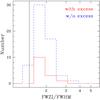 |
Fig. 2 Distributions of the ratio FWZI/FWHM of the SiO(2–1) line for the sources with (red solid histogram) and without (blue dashed histogram) Lyman excess. The FWZI is measured at 25% of the line peak (see text). The vertical line denotes the value of the ratio expected for a Gaussian profile. The bin size has been chosen following the Freedman-Diaconis rule. |
3.2. Infall
To determine the presence of infall, we adopted the approach of Mardones et al. (1997). Their method is based on the fact that an optically thick line of a molecule tracing infall, such as HCO+, has an asymmetric profile caused by redshifted self-absorption. In contrast, a line of the isotopolog, H13CO+, being optically thin, has a Gaussian profile. Therefore, by comparing the peak velocities of the two isotopologs, it is possible to reveal the presence of infall. In practice, Mardones et al. (1997) defined the parameter  (1)where Vthick is the peak velocity of the HCO+(1–0) line and Vthin and ΔVthin are, respectively, the peak velocity and FWHM of the H13CO+(1–0) line. Infall and expansion correspond to δV<0 and δV>0, respectively.
We computed δV for 171 of our sources, 56 of these with Lyman excess. The remaining 29 objects were not detected in the H13CO+ line or presented complex spectra made of multiple components and/or were affected by deep absorption features. The distributions of δV for the two samples are shown in Fig. 3. The step of the histograms has been taken equal to the mean 6σ uncertainty on the δV parameter. The distribution of the Lyman-excess sources is skewed toward negative values of δV, whereas the other appears centered on δV = 0. The Kolmogorov-Smirnov test gives a probability of only 3% that the two distributions are equivalent.
To further support that the Lyman-excess sample is dominated by infalling sources, we again followed Mardones et al. (1997), who defined the parameter  (2)where Ninfall is the number of sources with δV< −3σ (1σ rms in δV is ~0.05), Nexpansion those with δV> + 3 σ, and Ntotal = 171 the number of all sources. Positive values of E denote samples characterized by infalling objects, while negative values are associated with outflows. For the Lyman-excess sources we find E = 0.32 ± 0.09, whereas the other sample has E = 0.10 ± 0.06, consistent with the Lyman-excess sources being significantly more associated with infall than the others. In Table 1 we provide a summary of the information on the presence of infall in our sources.
Based on the above, we conclude that our findings are consistent with the accretion scenario proposed to explain the Lyman excess. Here a caveat is in order. Our HCO+ measurements are sensitive to large-scale (≲1 pc) infall and not to accretion onto the star or a putative circumstellar disk. The presence of infall is thus not direct evidence of the existence of accretion. However, we believe it plausible that at least part of the infalling material is bound to become focused on a very small region and there dissipate its energy in shocks.
4. Discussion and conclusions
The existence of Lyman excess in young early-type stars may have important consequences not only on the structure and evolution of H ii regions, but also on our understanding of the high-mass star formation process itself. All theories appear to agree that even the most massive stars may form through accretion, despite the different mechanisms invoked by the different models, such as competitive accretion (Bonnell et al. 2006) and monolithic collapse (Krumholz et al. 2009). However, it is still unclear whether the star reaches the ZAMS at approximately its final mass, or if still grows after igniting hydrogen burning.
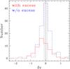 |
Fig. 3 Distributions of the Mardones et al. (1997) parameter, δV, for sources with (red solid histogram) and without (blue dashed histogram) Lyman excess. The hashed area indicates the range inside which | δV | < 3σ. Note how the solid distribution is skewed towards negative values of δV. |
Assuming that each of the H ii region is associated with a single massive star, our findings appear to support the latter scenario, where accretion may continue through the ionized region enshrouding the star, consistent with the model by Keto (2003; 2007). We can also conclude that the material accreted in this phase is a non-negligible fraction of the final stellar mass. If one-third of the ultracompact H ii regions are in the accretion phase, this means that accretion continues during one-third of the ultracompact H ii region lifetime (~105 yr; Wood & Churchwell 1989b), namely ~ 3 × 10⁴ yr. At an accretion rate of 10-4–10-3 M⊙ yr-1, typical of massive young stellar objects (see, e.g., Fazal et al. 2008 and references therein), this corresponds to a total accreted mass of 3–30 M⊙, a significant fraction of the mass of an early-type star. All the above indirectly suggests that the accretion flow significantly deviates from spherical symmetry. High accretion rates should quench the formation of an H ii region (Yorke 1984; Walmsley 1995; Keto 2002), but if accretion is focused through a circumstellar disk, for instance, the Lyman-continuum photons may escape along the disk axis and hence ionize the surrounding gas. This could explain the co-existence of accretion onto the star and formation of a compact H ii region in the same object.
The scenario depicted above assumes that our H ii regions are ionized by single stars. However, massive stars form in clusters (e.g., Tan et al. 2014), and it is likely that multiple stars contribute to the ionization. Therefore, an alternative scenario is that the infalling material does not end up on the ionizing, ZAMS star, but on one or more stellar companions still in the main accretion phase. In this case, our findings would imply that the high-mass star formation process in the cluster does not come to an end once the most massive star has reached the ZAMS, but instead continues even after the formation of an H ii region. Whether splitting the accreting material among two or more stars will be efficient enough to produce the required excess of Lyman-continuum photons is a non-trivial question that requires a dedicated model to be answered.
While all the previous considerations are at present purely speculative, direct detection of the accretion flow both in the molecular gas and in the ionized gas in the stellar surroundings are needed to establish the origin of the Lyman excess on solid grounds and to decide whether accretion is focused onto a single star or distributed among multiple stellar companions. To shed light on these questions, observations with the Atacama Large Millimeter and submillimeter Array (ALMA) are in progress for a selected subsample of our targets.
The GILDAS software has been developed at IRAM and Observatoire de Grenoble – see http://www.iram.fr/IRAMFR/GILDAS
Acknowledgments
It is a pleasure to thank the staff of the 30 m telescope for their valuable support during the observations. The research leading to these results has received funding from the European Commission Seventh Framework Programme (FP/2007–2013) under grant agreement No. 283393 (RadioNet3).
References
- Bonnell, I. A., & Bate, M. R. 2006, MNRAS, 370, 488 [NASA ADS] [CrossRef] [Google Scholar]
- Carter, M., Lazareff, B., Maier, D., et al. 2012, A&A, 538, A89 [NASA ADS] [CrossRef] [EDP Sciences] [Google Scholar]
- Cesaroni, R., Pestalozzi, M., Beltrán, M. T., et al. 2015, A&A, 579, A71 (C2015) [NASA ADS] [CrossRef] [EDP Sciences] [Google Scholar]
- Fazal, F. M., Sridharan, T. K., Qiu, K., et al. 2008, ApJ, 688, L41 [NASA ADS] [CrossRef] [Google Scholar]
- Hoare, M. G., Purcell, C. R., Churchwell, E. B., et al. 2012, PASP, 124, 939 [NASA ADS] [CrossRef] [Google Scholar]
- Hosokawa, T., & Omukai, K. 2009, ApJ, 691, 823 [NASA ADS] [CrossRef] [Google Scholar]
- Keto, E. H. 2002, ApJ, 580, 980 [NASA ADS] [CrossRef] [Google Scholar]
- Keto, E. H. 2003, ApJ, 599, 1196 [NASA ADS] [CrossRef] [Google Scholar]
- Keto, E. H. 2007, ApJ, 666, 976 [NASA ADS] [CrossRef] [Google Scholar]
- Klein, B., Hochgürtel, S., Krämer, I., et al. 2012, A&A, 542, L3 [NASA ADS] [CrossRef] [EDP Sciences] [Google Scholar]
- Krumholz, M. R., Klein, R. I., McKee, C. F., Offner, S. S. R., & Cunningham, A. J. 2009, Science, 323, 754 [NASA ADS] [CrossRef] [PubMed] [Google Scholar]
- López-Sepulcre, A., Cesaroni, R., & Walmsley, C. M. 2010, A&A, 517, A66 [NASA ADS] [CrossRef] [EDP Sciences] [Google Scholar]
- López-Sepulcre, A., Walmsley, C. M., Cesaroni, R., et al. 2011, A&A, 526, L2 [NASA ADS] [CrossRef] [EDP Sciences] [Google Scholar]
- Mardones, D., Myers, P. C., Tafalla, M., et al. 1997, ApJ, 489, 719 [NASA ADS] [CrossRef] [Google Scholar]
- Martins, F., Schaerer, D., & Hillier, D. J. 2005, A&A, 436, 1049 [NASA ADS] [CrossRef] [EDP Sciences] [Google Scholar]
- Molinari, S., Swinyard, B., Bally, J., et al. 2010, PASP, 122, 314 [NASA ADS] [CrossRef] [Google Scholar]
- Panagia, N. 1973, AJ, 78, 929 [NASA ADS] [CrossRef] [Google Scholar]
- Pilbratt, G. L., Riedinger, J. R., Passvogel, T., et al. 2010, A&A, 518, L1 [CrossRef] [EDP Sciences] [Google Scholar]
- Purcell, C. R., Hoare, M. G., Cotton, W. D., et al. 2013, ApJS, 205, 1 [NASA ADS] [CrossRef] [Google Scholar]
- Sánchez-Monge, Á., Beltrán, M. T., Cesaroni, R., et al. 2013, A&A, 550, A21 [NASA ADS] [CrossRef] [EDP Sciences] [Google Scholar]
- Schraml, J., & Mezger, P. G. 1969, ApJ, 156, 269 [NASA ADS] [CrossRef] [Google Scholar]
- Smith, M. D. 2014, MNRAS, 438, 1051 [NASA ADS] [CrossRef] [Google Scholar]
- Tan, J. C., Beltrán, M. T., Caselli, P., et al. 2014, Protostars and Planets VI, eds. H. Beuther, R. S. Klessen, C. P. Dullemond, & Th. Henning (Tucson: Univ. of Arizona Press), 149 [Google Scholar]
- Wood, D. O. S., & Churchwell, E. 1989a, ApJS, 69, 831 [NASA ADS] [CrossRef] [Google Scholar]
- Wood, D. O. S., & Churchwell, E. 1989b, ApJ, 340, 265 [NASA ADS] [CrossRef] [Google Scholar]
- Walmsley, M. 1995, in Rev. Mex. Astron. Astrofis. Ser. Conf., 1, Circumstellar Disks, Outflows, and Star Formation, eds. S. Lizano, & J. M. Torrelles, 137 [Google Scholar]
- Yorke, H. 1984, Workshop on Star Formation, ed. R. D. Wolstencroft (Edinburgh: Publ. R. Obs. Edinburgh), 63 [Google Scholar]
- Yorke, H. W., & Bodenheimer, P. 1999, ApJ, 525, 330 [NASA ADS] [CrossRef] [Google Scholar]
All Tables
Number of targets detected in the different tracers and corresponding detection rates.
All Figures
|
Fig. 1 Lyman-continuum photon rate versus the corresponding bolometric luminosity for the 200 CORNISH H ii regions with Herschel/Hi-GAL counterparts studied by C2015. The spectral types indicated at the top are computed under the assumption that Lbol originates from a single ZAMS star. The red solid line denotes the NLy–Lbol relation expected if the H ii regions were powered by single ZAMS stars (see C2015). Note that 67 objects (~34% of the sample) lie above this line. The error bars in the bottom right corner correspond to a 20% calibration uncertainty. |
| In the text | |
|
Fig. 2 Distributions of the ratio FWZI/FWHM of the SiO(2–1) line for the sources with (red solid histogram) and without (blue dashed histogram) Lyman excess. The FWZI is measured at 25% of the line peak (see text). The vertical line denotes the value of the ratio expected for a Gaussian profile. The bin size has been chosen following the Freedman-Diaconis rule. |
| In the text | |
|
Fig. 3 Distributions of the Mardones et al. (1997) parameter, δV, for sources with (red solid histogram) and without (blue dashed histogram) Lyman excess. The hashed area indicates the range inside which | δV | < 3σ. Note how the solid distribution is skewed towards negative values of δV. |
| In the text | |
Current usage metrics show cumulative count of Article Views (full-text article views including HTML views, PDF and ePub downloads, according to the available data) and Abstracts Views on Vision4Press platform.
Data correspond to usage on the plateform after 2015. The current usage metrics is available 48-96 hours after online publication and is updated daily on week days.
Initial download of the metrics may take a while.