| Issue |
A&A
Volume 588, April 2016
|
|
|---|---|---|
| Article Number | A128 | |
| Number of page(s) | 22 | |
| Section | Catalogs and data | |
| DOI | https://doi.org/10.1051/0004-6361/201527641 | |
| Published online | 30 March 2016 | |
Exploring the crowded central region of ten Galactic globular clusters using EMCCDs
Variable star searches and new discoveries⋆,⋆⋆
1 SUPA, School of Physics and Astronomy, University of St. Andrews, North Haugh, St Andrews, KY16 9SS, UK
e-mail: This email address is being protected from spambots. You need JavaScript enabled to view it.
2 European Southern Observatory, Karl-Schwarzschild-Straße 2, 85748 Garching bei München, Germany
3 Qatar Environment and Energy Research Institute (QEERI), HBKU, Qatar Foundation, Doha, Qatar
e-mail: This email address is being protected from spambots. You need JavaScript enabled to view it.
4 Centre for Electronic Imaging, Dept. of Physical Sciences, The Open University, Milton Keynes MK7 6AA, UK
5 Niels Bohr Institute and Centre for Star and Planet Formation, University of Copenhagen, Øster Voldgade 5, 1350 Copenhagen K, Denmark
6 Space Telescope Science Institute, 3700 San Martin Drive, Baltimore, MD 21218, USA
7 Dipartimento di Fisica “E. R. Caianiello”, Università di Salerno, via Giovanni Paolo II 132, 84084 - Fisciano (SA), Italy
8 Istituto Nazionale di Fisica Nucleare, Sezione di Napoli, Napoli, Italy
9 NASA Exoplanet Science Institute, MS 100-22, California Institute of Technology, Pasadena CA 91125, USA
10 Istituto Internazionale per gli Alti Studi Scientifici (IIASS), 84019 Vietri Sul Mare (SA), Italy
11 Max Planck Institute for Astronomy, Königstuhl 17, 69117 Heidelberg, Germany
12 Yunnan Observatories, Chinese Academy of Sciences, 650011 Kunming, PR China
13 Key Laboratory for the Structure and Evolution of Celestial Objects, Chinese Academy of Sciences, 650011 Kunming, PR China
14 Korea Astronomy and Space Science Institute, 305-348 Daejeon, Republic of Korea
15 Finnish Centre for Astronomy with ESO (FINCA), University of Turku, Väisäläntie 20, 21500 Piikkiö, Finland
16 Instituto de Astrofísica, Facultad de Física, Pontificia Universidad Católica de Chile, Av. Vicuña Mackenna 4860, 7820436 Macul, Santiago, Chile
17 Department of Physics, Sharif University of Technology, PO Box 11155-9161, Tehran, Iran
18 Astronomisches Rechen-Institut, Zentrum für Astronomie der Universität Heidelberg, Mönchhofstr. 12-14, 69120 Heidelberg, Germany
19 Planetary and Space Sciences, Department of Physical Sciences, The Open University, Milton Keynes, MK7 6AA, UK
20 Max-Planck-Institute for Solar System Research, Justus-von-Liebig-Weg 3, 37077 Göttingen, Germany
21 Astrophysics Group, Keele University, Staffordshire, ST5 5BG, UK
22 Las Cumbres Observatory Global Telescope Network, 6740 Cortona Drive, Suite 102, Goleta, CA 93117, USA
23 Institut d’Astrophysique et de Géophysique, Université de Liège, Allée du 6 Août, Bât. B5c, 4000 Liège, Belgium
Received: 26 October 2015
Accepted: 22 December 2015
Abstract
Aims. We aim to obtain time-series photometry of the very crowded central regions of Galactic globular clusters; to obtain better angular resolution thanhas been previously achieved with conventional CCDs on ground-based telescopes; and to complete, or improve, the census of the variable star population in those stellar systems.
Methods. Images were taken using the Danish 1.54-m Telescope at the ESO observatory at La Silla in Chile. The telescope was equipped with an electron-multiplying CCD, and the short-exposure-time images obtained (ten images per second) were stacked using the shift-and-add technique to produce the normal-exposure-time images (minutes). Photometry was performed via difference image analysis. Automatic detection of variable stars in the field was attempted.
Results. The light curves of 12 541 stars in the cores of ten globular clusters were statistically analysed to automatically extract the variable stars. We obtained light curves for 31 previously known variable stars (3 long-period irregular, 2 semi-regular, 20 RR Lyrae, 1 SX Phoenicis, 3 cataclysmic variables, 1 W Ursae Majoris-type and 1 unclassified) and we discovered 30 new variables (16 long-period irregular, 7 semi-regular, 4 RR Lyrae, 1 SX Phoenicis and 2 unclassified). Fluxes and photometric measurements for these stars are available in electronic form through the Strasbourg astronomical Data Center.
Key words: blue stragglers / galaxies: star clusters: general / globular clusters: general / stars: variables: RR Lyrae / novae, cataclysmic variables / instrumentation: high angular resolution
Based on data collected by the MiNDSTEp team with the Danish 1.54m telescope at ESO’s La Silla observatory in Chile.
Full Table 1 is only available at CDS via anonymous ftp to cdsarc.u-strasbg.fr (130.79.128.5) or via http://cdsarc.u-strasbg.fr/viz-bin/qcat?J/A+A/588/A128
Royal Society University Research Fellow.
Sagan visiting fellow.
© ESO, 2016
1. Introduction
Globular cluster systems in the Milky Way are excellent laboratories for several fields in astronomy, from cosmology to stellar evolution. As old as our Galaxy is, globular cluster systems are stellar fossils that enable astronomers to look back to earlier galaxy-formation stages to have a better understanding of the stellar population that forms the clusters.
Possibly the first official register of globular clusters started with the Catalog of Nebulae and Star Clusters made by Messier (1781) and followed by Herschel (1786). Several early studies (i.e. Barnard 1909; Hertzsprung 1915; Eddington 1916; Shapley 1916; Oort 1924) of globular clusters can also be found in the literature.
The first variable star found in the field of a globular cluster was T Scorpii (Luther 1860). Subsequent early studies of variable stars in globular clusters can also be found in the literature (see e.g. Davis 1917; Bailey 1918; Sawyer 1931; Oosterhoff 1938). Measurements of the variability of these stars were performed either by eye or by using photographic plates. It was not until about 1980 (Martínez Roger et al. 1999) that deeper studies in the photometry of globular clusters were performed using both CCDs and larger telescopes.
More recently, the implementation of new image analysis tools, such as difference image analysis (DIA; Alard & Lupton 1998), have enabled much more detailed and quantitative studies, but there are still several limiting constraints. The first is saturated stars. It is always important to balance the exposure time to prevent bright stars from saturating the CCD without losing signal-to-noise ratio (S/N) in the fainter stars. The second difficulty is the crowded nature of the central regions. Sometimes it is complicated to properly measure the point spread function (PSF) of the stars in the central regions of globular clusters owing to blending that is caused by the effect of atmospheric turbulence.
To overcome these limitations, we started a pilot study of the crowded central regions of globular clusters using electron-multiplying CCDs (EMCCDs) and the shift-and-add technique. The choice for our globular cluster sample is based mainly on the central concentration of stars while favouring clusters that are well known to have variable stars. We published the results of globular cluster NGC 6981 in Skottfelt et al. (2013) with the discovery of two new variables and five more globular clusters in Skottfelt et al. (2015a), where a total of 114 previously unknown variables were found. In this paper we report the results on ten further globular clusters.
Section 2 describes the instrumentation, data obtained, pipeline used and the data reduction procedures. Sections 3–5 explain the calibration, the colour magnitude diagrams, and the strategy used to identify variable stars. In Sect. 6 we classify the variable stars. Section 7 describes the methodology that was followed to observe the globular clusters. Section 8 presents the results that were obtained in each globular cluster and Sect. 9 summarises the main conclusions.
2. Data and reductions
2.1. Telescope and instrument
Observations were taken using the 1.54 m Danish telescope at the ESO observatory at La Silla in Chile, which is located at an elevation of 2340 m at 70°44′07 662W 29°15′14235S. The telescope is equipped with an Andor Technology iXon+897 EMCCD camera, which has a 512 × 512 array of 16 μm pixels, a pixel scale of 009 per pixel and a total field of view of ~45 × 45 arcsec2.
For this research, the camera was configured to work at a frame-rate of 10 Hz (this is 10 images per second) and an EM gain of 300e−/photon. The camera is placed behind a dichroic mirror, which works as a long-pass filter. Taking the mirror and the sensitivity of the camera into consideration, it is possible to cover a wavelength range of between 650 nm to 1050 nm, corresponding roughly to a combination of SDSS i′ + z′ filters (Bessell 2005). More details about the instrument can be found in Skottfelt et al. (2015b).
2.2. Observations
Observations were taken during 2013 and 2014 as part of an ongoing programme at the Danish telescope that was implemented from April to September each year. Figure 1 shows histograms of the number of observations per night per cluster. Data in the left-hand panel corresponds to 2013 and data in the right-hand panel, to 2014. As time at the telescope was limited, we tried to observe all clusters with the same rate as far as it was possible by taking two observations each night. However, as it is shown in the histograms, this was not possible because of the weather conditions or because the telescope was used to monitor microlensing events carried out by the MINDSTEp consortium, as part of the programme to characterise exoplanets.
It is worth commenting that, depending on the magnitude level of the horizontal branch of each globular cluster, observations with total exposure times between six to ten minutes were produced (see Sect. 7). To do this the camera was continuously taking images (at the rate of ten images per second) for the total exposure time desired and then all the images obtained during that particular exposure time were stacked to produce a single observation. That is, a ten-minute exposure time observation is the result of stacking 6000 images that were taken continuously. The technique for image stacking is called “shift-and-add” and it is explained in Sect. 2.3.2.
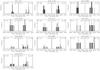 |
Fig. 1 Histograms with the number of observations per night for each globular cluster studied in this work. Panels on the left: plotted data taken during 2013; panels on the right: data taken during 2014. |
2.3. EMCCD data reduction
EMCCDs, also known as low-light-level charge-coupled devices (L3CCD; see e.g. Smith et al. 2008; Jerram et al. 2001), are conventional CCDs that are equipped with an extended serial gain register in which each electron produced during the exposure time has a probability of creating a second electron (avalanche multiplication) when it passes through the extended gain register. The process in which the second electrons are created is called impact ionisation.
To do bias, flat-field and tip-tilt corrections, the procedures and algorithms described in Harpsøe et al. (2012) were used.
2.3.1. Tip-tilt correction
As described in Harpsøe et al. (2012), the tip-tilt correction for a sample of bias and flat-field corrected images Ii(x,y) with respect to a reference image R(x,y) is calculated by finding the global maximum of Pi defined by Eq. (1),
![Mathematical equation: \begin{equation} \label{eq:tip_tilt} P_i(x,y)=|FFT^{-1}[FFT(R)\cdot\overline{FFT(I_i)}]|, \end{equation}](/articles/aa/full_html/2016/04/aa27641-15/aa27641-15-eq15.png) (1)which is the cross-correlation image (see Fourier cross-correlation theorem). The position of the maximum (xmax,ymax) is used to shift each of the images in the sample Ii(x,y) to the position of the stars in the reference image.
(1)which is the cross-correlation image (see Fourier cross-correlation theorem). The position of the maximum (xmax,ymax) is used to shift each of the images in the sample Ii(x,y) to the position of the stars in the reference image.
2.3.2. Image quality and stacking
The image quality is assessed by defining the quality index 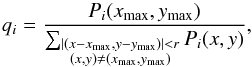 (2)which represents the ratio of the maximum Pi(xmax,ymax) to the sum of the Pi(x,y) values of the surrounding pixels. Once this index is calculated, images from a single observation are sorted from the one with the best quality (smallest qi) to the one with the worst quality (largest qi) and a ten-layer image frame is built by stacking images in the sequence: 1%, 2%, 5%, 10%, 20%, 50%, 90%, 98%, 99%, and 100%. This means that the first-layer frame has stacked the top 1% of the best quality images, the second-layer frame has stacked the next 1% of the best quality images, the third-layer frame has stacked the next 3%, the fourth has stacked the next 5%, and so on. In this study, we use the layers with the best full width at half maximun (FWHM) over all the frames to build the reference image for each globular cluster and we stack the ten layers of an observation into a single science image for the photometry (see also Skottfelt et al. 2015a).
2.4. Photometry
To extract the photometry in each of the images we used the DanDIA1 pipeline (Bramich 2008; Bramich et al. 2013), which is based on difference image analysis (DIA).
As commented in Sect. 2.3.2, for each EMCCD observation, we produced a ten-layer calibrated image cube where each of the images in the cube is sorted by quality. DanDIA builds a high S/N and high-resolution reference frame by selecting and combining the best quality images available in the cubes. This is done by detecting bright stars using DAOFIND (Stetson 1987) and employing these to align the images using the triangulation technique described in Pál & Bakos (2006). Each of the reference frames used in the analysis of each globular cluster can be found throughout the paper (e.g. Fig. 6) and the mean PSF FWHM for each reference image is listed in Table 3. Positions and reference fluxes (fref) in ADU/s for each star are calculated using the PSF photometry package “STARFINDER” (Diolaiti et al. 2000). The pipeline implements a low-order polynomial degree for the spatial variation of the PSF model (a quadratic polynomial degree was sufficient in our case).
Once the reference image is built, all of the science frames are registered with the reference image by once again using the Stetson (1987) and Pál & Bakos (2006) algorithms described before. Image subtraction then determines a spatially variable kernel, modelled as a discrete pixel array, that best matches the reference image to each science image. The photometric scale factor (p(t)) used to scale the reference frame to each image is calculated as part of the kernel model (Bramich et al. 2015). Difference images are created by subtracting the convolved reference image from each science image. Finally, difference fluxes (fdiff(t)) in ADU/s for each star detected in the reference image are measured in each of the difference images by optimally scaling the PSF model for the star to the difference image. The light curve for each star is the total flux (ftot(t)) in ADU/s defined as 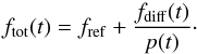 (3)We transform this to instrumental magnitudes mins at each given time t:
  (4)A detailed description of the procedures and techniques employed by the pipeline can be found in Bramich et al. (2011).
Time-series I photometry for all known and new variables in the field of view covered in each globular cluster.
 |
Fig. 2 Standard I magnitude taken from the HST observations as a function of the instrumental i′ + z′ magnitude. The red lines are the fits that best match the data and they are described by the equations in the titles of each plot. The correlation coefficient is 0.999 in all cases. |
For a conventional CCD, the noise model used by DanDIA is represented by the pixel variances  of the image k at the pixel positions i, j
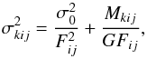 (5)where σ0 is the CCD readout noise (ADU), Fij is the master flat-field image, G is the CCD gain (e−/ADU) and Mkij is the image model. For an EMCCD, the noise model for a single exposure is different:
 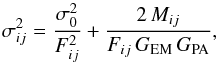 (6)where GEM is the electron-multiplying gain (photons/e−) and GPA is the Pre Amp gain (e−/ADU).
If N exposures are combined by summation, then the noise model for the combined image  is given by Eq. (7):
 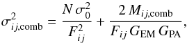 (7)where Mij,comb is the image model of the combined image (see also Skottfelt et al. 2015a).
In Table 1, we illustrate the format of the electronic table with all fluxes and photometric measurements as they are available at the CDS.
2.5. Astrometry and finding chart
To fit an astrometric model for the reference images, celestial coordinates available in the ACS Globular Cluster Survey2 (see Anderson et al. 2008) were uploaded for the field of the cluster through Gaia (Graphical Astronomy and Image Analysis Tool; Draper 2000). An (x,y) shift was applied to all of the uploaded positions until they matched the stars in the fields. Stars lying outside the field of view and those without a clear match were removed, and the (x,y) shift was refined by minimising the squared coordinate residuals. The number of stars used in the matching process ranged from 108 stars to 1034 stars, which guaranteed that the astrometric solutions that were applied to the reference images considered enough stars to cover the whole field. The radial rms scatter obtained in the residuals was ~01 (~1 pixel). The astrometrically calibrated reference images were used to produce a finding chart for each globular cluster on which we marked the positions and identifications of all variable stars studied in this work. Finally, a table with the equatorial J2000 celestial coordinates of all variables for each globular cluster is given (see, e.g. Table 4).
3. Photometric calibration
The photometric transformation of instrumental magnitudes to the standard system was accomplished using information available in the ACS Globular Cluster Survey, which provides calibrated magnitudes for selected stars in the fields of 50 globular clusters extracted from images taken with the Hubble Space Telescope (HST) instruments ACS and WFPC.
Convention used in the variable star classification of this work, based on the definitions of the general catalogue of variable stars (Samus et al. 2009a).
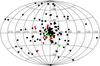 |
Fig. 3 Positions of the 157 known globular clusters in the Galaxy are plotted in the Galactic plane system. The 10 globular clusters studied in this work are labelled in red. Green corresponds to the globular clusters studied in Skottfelt et al. (2015a, 2013). |
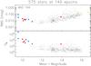 |
Fig. 4 Root mean square (rms) magnitude deviation (top) and SB statistic (bottom) versus the mean I magnitude for the 575 stars detected in the field of view of the reference image for NGC 104. Coloured points follow the convention adopted in Table 2 to identify the types of variables found in the field of this globular cluster. |
By matching the positions of the stars in the field of the HST images with those in our reference images, we obtained photometric transformations for our ten globular clusters, as shown in Fig. 2. The I magnitude obtained from the ACS (see Sirianni et al. 2005) is plotted versus the instrumental i′ + z′ magnitude obtained in this study. The red lines are linear fits with slope unity yielding zero-points labelled in the title of each plot. N is the number of stars used in the fit. The correlation coefficient was 0.999 in all cases. A transformation was derived for each globular cluster.
Some of the physical properties of the globular clusters studied in this work.
4. Colour magnitude diagrams
As our sample has data available for only one filter, we decided to build colour magnitude diagrams (CMD; see Fig. 5) by using the information available from the HST images at the ACS Globular Cluster Survey. The data used correspond to the V and I photometry obtained in Sirianni et al. (2005). The CMD was useful in classifying the variable stars, especially those with poorly defined light curves such as long-period irregular variables and semi-regular variables, as well as corroborating cluster membership.
5. Variable star searches
During the reductions, the DanDIA pipeline produced a total of 12 541 light curves for stars in the cores of the ten globular clusters studied. We used three automatic (or semi-automatic) techniques to search for variable stars, as described in Sects. 5.1−5.3.
5.1. Root mean square
Diagrams of root mean square (rms) magnitude deviation against mean I magnitude (see top Fig. 4) were constructed for each globular cluster. In these diagrams, we measure not only the photometric scatter for each star studied in this work, but also the intrinsic variation of the variable stars over time, which gives them a higher rms than the non-variables. The classification is indicated by colour, as detailed in Table 2.
To select possible variable stars, we fit a polynomial model to the rms values as a function of magnitude and flag all stars with rms values greater than three times the model. All difference images obtained with DanDIA were blinked as well to corroborate the variation of the stars selected.
5.2. SB statistic
A detailed discussion can be found about the benefits of using the SB statistic to detect variable stars (Figuera Jaimes et al. 2013) and RR Lyrae with Blazhko effect (Arellano Ferro et al. 2012). The SB statistic is defined as  (8)where N is the number of data points for a given light curve and M is the number of groups formed of time-consecutive residuals of the same sign from a constant-brightness light curve model (e.g. mean or median). The residuals ri,1 to ri,ki correspond to the ith group of ki time-consecutive residuals of the same sign with corresponding uncertainties σi,1 to σi,ki. The SB statistic is larger in value for light curves with long runs of consecutive data points above or below the mean, which is the case for variable stars with periods longer than the typical photometric cadence. Plots of SB versus mean I magnitude are given for each globular cluster (see bottom Fig. 4) and variable stars are plotted in colour.
To select variable stars, the same technique employed in 5.1 was used, but in this case the threshold was shifted between 3−10 times the model SB values, depending on the distribution of the data in each globular cluster. All stars selected were inspected in the difference images in the same way as explained in Sect. 5.1.
5.3. Stacked difference images
NGC 104: ephemerides and main characteristics of the variable stars in the field of this globular cluster.
Based on the results obtained using the DanDIA pipeline, a stacked difference image was built for each globular cluster with the aim of detecting the difference fluxes that correspond to variable stars in the field of the reference image. The stacked image is the result of summing the absolute values of the difference images divided by the respective pixel uncertainty  (9)where Sij is the stacked image, Dkij is the kth difference image, σkij is the pixel uncertainty associated with each image k and the indexes i and j correspond to pixel positions.
All of the variable star candidates obtained by using the rms diagrams or the SB statistic explained in Sects. 5.1 and 5.2 were inspected visually in the stacked images to confirm or refute their variability. Difference images were also blinked to finally corroborate the variation of the stars selected.
6. Variable star classification
All variable stars found were plotted in the colour–magnitude diagram for the corresponding globular cluster, to have a better understanding of the nature of their variation and their cluster membership. A period search of the light curve variations was undertaken by using the string method (Lafler & Kinman 1965) and by minimising the χ2 in a Fourier analysis fit. To decide the classification of the variable stars, we used the conventions defined in the General Catalogue of Variable Stars (Samus et al. 2009a) and by considering their position in the colour–magnitude diagrams and the periods found.
In Table 2, the classification, corresponding symbols, and colours used in the plots throughout the paper are shown.
7. Globular clusters observed
Figure 3 shows the Galactic plane celestial coordinates (l,b) for the 157 globular clusters listed in (Harris 1996, 2010 edition). The ten globular clusters analysed in this work are plotted in red where six are in the southern hemisphere and four are in the northern hemisphere. Also plotted (in green) are the six globular clusters studied in Skottfelt et al. (2015a, 2013).
NGC 5139: ephemerides and main characteristics of the variable stars in the field of this globular cluster.
The strategy to select and observe the clusters was the following:
-
(1)
We took into account the visibility. We selected all visible globular clusters based on the geographical coordinates of the telescope and some pointing restrictions too.
-
(2)
We focused on the concentration of stars in the central region of the clusters. As reference, we used the central luminosity density ρ0 (L⊙ pc-3) listed in (Harris 1996, 2010 edition). The entire sample, which is available in the catalogue, has log (ρ0) from ~0 to ~6. To explore the potential of the EMCCD and the shift-and-add technique for photometry, a sample with different levels of ρ0 were chosen from a very dense cluster NGC 6752 (log (ρ0) = 5.04) to a less dense cluster NGC 6723 (log (ρ0) = 2.79) and some intermediate levels as NGC 5139 (log (ρ0) = 3.15) and NGC 5286 (log (ρ0) = 4.10).
-
(3)
A bibliography review revealed how many variable stars are known from previous work. To do this, we used the information available for each globular cluster in the Catalogue of Variable Stars in Galactic Globular Clusters (Clement et al. 2001) and the ADS to do the bibliography review up-to-now.
-
(4)
Exploration of known colour–magnitude diagrams. As most of the variable stars that are globular cluster members have a particular position in these diagrams, we focused our attention on globular clusters with a high concentration of stars, for example at the top of the red giant branch (for semi-regular variables), the instability strip of the horizontal branch (for RR Lyrae), and the blue straggler region (for SX Phoenicis). To do this we used the colour information available in the ACS to build colour–magnitude diagrams for each globular cluster. Additionally, we also used the Galactic globular clusters database3.
-
5)
The exposure time to be used for a single EMCCD observation for each globular cluster was chosen based on the V magnitude of the horizontal branch. We selected exposure times as follows:
6 min for VHB< 14 mag,
8 min for 14 mag < VHB< 17 mag,
10 min for VHB> 17 mag.
We chose the ten globular clusters presented in this work. Some of their most relevant physical properties are detailed in Table 3.
8. Results
8.1. NGC 104/C0021-723/47 Tucanae
The globular cluster was discovered by Nicholas Louis de Lacaille in 17514. The cluster is in the constellation of Tucana at a distance of 4.5 kpc from the Sun and 7.4 kpc from the Galactic centre. It has a metallicity of [Fe/H] = −0.72 dex and a distance modulus of (m−M)V = 13.37 mag. The magnitude of its horizontal branch is VHB = 14.06 mag.
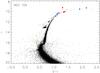 |
Fig. 5 Colour magnitude diagram for the globular cluster NGC 104 built with V and I magnitudes available in the ACS globular cluster survey extracted from HST images. The variable stars are plotted in colour following the convention adopted in Table 2. |
In Fig. 4, the root mean square magnitude deviation (top) and SB statistic (bottom) are plotted versus the mean I magnitude for a total of 575 light curves that were extracted in this analysis. The coloured points correspond to the variable stars studied in this work compared to the stars where no variation is found (normal black points).
8.1.1. Known variables
This globular cluster has approximately 300 known variable sources in the Catalogue of Variable Stars in Galactic Globular Clusters (version of summer 2007; Clement et al. 2001), which include long-period irregular variables, SX Phoenicis, RR Lyrae, and binary systems. Most were found by Albrow et al. (2001), Weldrake et al. (2004), and Lebzelter & Wood (2005). There are also 20 millisecond pulsars listed in the literature for this cluster (Freire et al. 2001). However, no visual counterparts have been found at their positions.
In the field of view covered by the reference image (Fig. 6), there are 49 previously known variables. However, for this cluster we were only able to detect stars brighter than I = 16.1 mag (see rms in Fig. 4). As a result, five known variable stars, which were brighter than this limit, were detected. These stars are labelled in the literature as PC1-V12, WF2-V34, LW10, LW11, and LW12. Our light curves for these variables can be found in Fig. 7.
PC1-V12: this star was discovered by Albrow et al. (2001) and classified as a blue straggler star (BSS) with an average magnitude of V = 16.076 mag. No period was reported in this case and it was not possible to find a period for this star in the present work.
WF2-V34: the variability of this star was discovered by Albrow et al. (2001) and was classified as a semi-regular variable with a period of P = 5.5 d. However, using this period it was not possible to produce a good phased light curve and it was not possible to find another period for this star. Based on this, we classified this star as a long-period irregular variable.
LW10-LW12: these three stars were discovered by Lebzelter & Wood (2005). Their positions in the colour–magnitude diagram (Fig. 5) confirm their cluster membership. Lebzelter & Wood (2005) classified them as long-period irregular variables and suggested periods for these stars to be LW10: 110 d or 221 d, LW11: 36.0 d, and LW12 : 61 d or 116 d. However, LW10 and LW12 are clearly irregular variables (see our Figs. 7 and 1 from Lebzelter & Wood 2005). For LW11 we found a period of 19.37 d and we classify it as semi-regular.
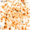 |
Fig. 6 Finding chart for the globular cluster NGC 104. The image used corresponds to the reference image constructed during the reduction. All known variables and new discoveries are labelled. Image size is ~41 × 41 arcsec2. |
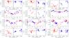 |
Fig. 7 NGC 104: light curves of the known and new variables discovered in this globular cluster. Red triangles correspond to the data obtained during the year 2013 and blue circles correspond to the data obtained during the year 2014. For EM7, we plot the quantity fdiff(t) /p(t) since a reference flux is not available. |
8.1.2. New variables
After extracting and analysing all possible variable sources in the field of our images, a total of seven new variables (EM1-EM7) were found of which four are semi-regular variables, two are long-period irregular variables and one is unclassified.
For this cluster, the nomenclature employed for most of the variable stars discovered in previous works does not correspond to the typical numbering system (e.g. V1, V2, V3, ... , Vn). For example, variables discovered by Lebzelter & Wood (2005) and Weldrake et al. (2004) are numbered using their initials LW and W, respectively; Albrow et al. (2001) used a PC or WF nomenclature that makes reference to the instrument employed during the observations. As a result, we did not find it practical to assign the typical numbering system to the new variable stars discovered in this work and we decided to use as reference the EMCCD camera used in the observations. That is, new variables are numbered as EM1-EM7.
EM1-EM4: these variable stars are placed at the top of the colour magnitude diagram (Fig. 5). Their light curve shape, amplitudes and periods found suggest that these stars are semi-regular variables. Periods found for these variables are listed in Table 4. The star EM1 is not over the red giant branch in Fig. 5 but instead is more towards the asymptotic giant branch, appearing at the top on the left. Finally the star EM4 is located at the bottom part of the red giant branch just below the starting point of the horizontal branch.
EM5-EM6: these stars have amplitudes of ~0.06 and 0.07 mag, respectively. They are located at the top of the red giant branch. We were not able to determine a proper period for these stars. Consequently, we classified them as long-period irregular variables.
EM7: this star is placed in the blue straggler region. The variation in the difference images is clear for this star. However, the pipeline did not find this star in the reference image and no reference flux is available to convert the difference fluxes to magnitudes. The difference fluxes are plotted in Fig. 7. We were unable to determine a period.
8.2. NGC 5139/C1323-472/ Omega Centauri
This globular cluster was discovered by Edmond Halley in 16775. The cluster is in the constellation of Centaurus at 5.2 kpc from the Sun and 6.4 kpc from the Galactic centre. It has a metallicity of [Fe/H] = −1.53 dex, a distance modulus of (m−M)V = 13.94 mag and the level of the horizontal branch is at VHB = 14.51 mag.
8.2.1. Known variables
In the Catalogue of Variable Stars in Galactic Globular Clusters (Clement et al. 2001), there are approximately 400 variable stars for this globular cluster. Most of these variables were discovered by Bailey (1902), Kaluzny et al. (2004) and Weldrake et al. (2007). All of the known variables are outside the field of view of our reference image. Most recently, Navarrete et al. (2015) made an updated analysis of the variables in this cluster, but the variables in their study are also located outside the field of view of our reference image.
8.2.2. New variables
We found three new variables in this globular cluster. Two are long-period irregular variables and one is unclassified.
The new variable stars are plotted in the rms diagram and SB statistic (see Fig. 8). Based on the position of the stars in Figs. 8 and 9, there is no evidence of RR Lyrae in the field covered by this work or in the inspection of the difference images obtained in the reductions.
V457: this variable star has an amplitude of ~0.15 mag with a median magnitude I = 15.82 mag. It lies on the RGB and we were unable to find a period.
V458, V459: theses two stars are at the top of the red giant branch in Fig. 9 and have amplitudes of ~0.04 and ~0.06 mag, respectively. No periods were found in this work. V459 is on the red side of the main red giant branch. We classify them as long-period irregular variables.
8.3. NGC 5286/C1343-511/Caldwell 84
This globular cluster was discovered by James Dunlop in 1827 (O’Meara 2002). It is in the constellation of Centaurus at 11.7 kpc from the Sun and 8.9 kpc from the Galactic centre. It has a metallicity of [Fe/H] = −1.69 dex, a distance modulus of (m−M)V = 16.08 mag, and the magnitude level of the horizontal branch is at VHB = 16.63 mag.
In Fig. 12, the rms diagram and the SB statistic are shown for the sample of 1903 stars that were analysed in this globular cluster. Most of them have 74 epochs. All variable stars studied in this work are plotted using the colour classification given in Table 2.
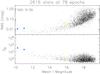 |
Fig. 8 Root mean square (rms) magnitude deviation (top) and SB statistic (bottom) versus the mean I magnitude for the 2616 stars detected in the field of view of the reference image for NGC 5139. Coloured points follow the convention adopted in Table 2 to identify the types of variables found in the field of this globular cluster. |
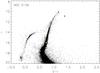 |
Fig. 9 Colour magnitude diagram of the globular cluster NGC 5139 built with V and I magnitudes available in the ACS globular cluster survey extracted from HST images. The variable stars are plotted in colour following the convention adopted in Table 2. |
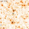 |
Fig. 10 Finding chart for the globular cluster NGC 5139. The image used corresponds to the reference image constructed during the reduction. The new variables discovered are labelled. Image size is ~41 × 41 arcsec2. |
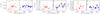 |
Fig. 11 NGC 5139: light curves of the three new variables discovered in this globular cluster. Symbols are the same as in Fig. 7. |
NGC 5286: ephemerides and main characteristics of the variable stars in the field of this globular cluster.
NGC 6093: ephemerides and main characteristics of the variable stars in the field of this globular cluster.
8.3.1. Known variables
This globular cluster has 58 known variable stars listed in the Catalogue of Variable Stars in Galactic Globular Clusters (Clement et al. 2001) of which 52 are RR Lyrae stars. There are only 11 previously known variable stars in the field of view of our reference image (V37, V39, V40, V41, V43, V46, V50, V55, V56, V57, V58). All of them are RR Lyrae, which were discovered by Zorotovic et al. (2010) using DIA on imaging data from a one-week observing run.
The celestial coordinates given in Table 1 of Zorotovic et al. (2010) do not match the positions of the known variable stars in the field of our images. We therefore used the finding chart given in their Fig. 1 to do a visual matching of the variables. As pointed out in the Catalogue of Variable Stars in Galactic Globular Clusters (Clement et al. 2001), there is a difference in the position of the variables studied by Zorotovic et al. (2010) with respect to the position of the variables in Samus et al. (2009b), which is ~6 arcsec in declination and ≲1 arcsec in right ascension. This difference is corroborated by the position of the variables in our reference image. Celestial coordinates of the positions we used are given in Table 6.
Our extended observational baseline has allowed us to greatly improve the periods of the variables discovered by Zorotovic et al. (2010). Our period estimates are listed in Table 6 and have typical errors of 0.00002−0.00010 d. We confirm the variable star classifications made by Zorotovic et al. (2010). We note that V41 is a strong blend with a brighter star that is only just resolved in our high-resolution reference image.
8.3.2. New variables
In this globular cluster we found 11 previously unknown variables where five are long-period irregular variables, three are semi-regular variables, two are RR Lyrae, and one is an SX Phoenicis.
V63: the star has a median magnitude of I ~ 18.52 mag and is in the blue straggler region. Its amplitude is Ai′ + z′ ~0.49 mag and it has a period of P = 0.0486320 d. The star is clearly an SX Phoenicis. The variation of this star was not detected using the rms or SB statistic, although it is very clear in the difference images.
V64: this star is an RR Lyrae pulsating in the first overtone (RR1) with a period of 0.369783 d and an amplitude of 0.41 mag. In Fig. 14, it is clear that V64 is very close to a bright star (6.808 pixels or 0.613 arcsec). This could be the reason why this variable was not discovered before and makes a good example of the benefits of using the EMCCD cameras and the shift-and-add technique along with DIA.
V65: this star is another RR Lyrae which is pulsating in the fundamental mode (RR0) with a period of 0.619491 d and an amplitude of ~0.36 mag.
V66-V68: these stars are semi-regular variables. As can be seen in Fig. 13, they are at the top of the red giant branch. They have amplitudes that range between 0.04 to 0.10 mag. They have periods between ~17 to 33 d. Ephemerides for these stars can be found in Table 6.
V69-V73: these five stars are also positioned at the top of the red giant branch with amplitudes of 0.05 to 0.52 mag. It was not possible to find periods for these stars in this work. Consequently, they were classified as long-period irregular variables.
In Fig. 16 the amplitude-period diagram for the RR Lyrae stars studied in this cluster is shown. The filled lines correspond to the Oosterhoff type I (OoI) and the dashed lines correspond to the Oosterhoff type II (OoII) models defined by Kunder et al. (2013). All RR0 variables (with the exception of V65) fall into the model for OoII type while the RR1 stars scatter around both models. In this diagram the RR0 stars suggest an OoII type classification for NGC 5286, which is in agreement with the study done by Zorotovic et al. (2010) where they found that their research pointed to an OoII status as well.
8.4. NGC 6093/C1614-228/M 80
This globular cluster was discovered by Charles Messier in 17816. This cluster is in the constellation of Scorpius at 10.0 kpc from the Sun and 3.8 kpc from the Galactic centre. Its has a metallicity of [Fe/H] = −1.75 dex, a distance modulus of (m−M)V = 15.56 mag and the position of its horizontal branch is at V = 16.10 mag.
A total of 1220 light curves were extracted in the field covered by the reference image for the globular cluster NGC 6093. Most of the stars have 58 epochs in their light curves and variable stars studied in this work are plotted with colour in the rms and SB diagrams shown in Fig. 17.
NGC 6121: ephemerides and main characteristics of one variable star in the field of this globular cluster.
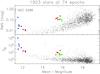 |
Fig. 12 Root mean square (rms) magnitude deviation (top) and SB statistic (bottom) versus the mean I magnitude for the 1903 stars detected in the field of view of the reference image for NGC 5286. Coloured points follow the convention adopted in Table 2 to identify the types of variables found in the field of this globular cluster. |
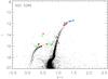 |
Fig. 13 Colour magnitude diagram for the globular cluster NGC 5286 built with V and I magnitudes available in the ACS globular cluster survey extracted from HST images. The variable stars are plotted in colour following the convention adopted in Table 2. |
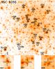 |
Fig. 14 Finding chart for the globular cluster NGC 5286. The image used corresponds to the reference image constructed during the reduction. All known variables and new discoveries are labelled. Image size is ~41 × 41 arcsec2. The image stamps are of size ~4.6 × 4.6 arcsec2. |
8.4.1. Known variables
This globular cluster has 34 known variable sources in the Catalogue of Variable Stars in Galactic Globular Clusters (Clement et al. 2001). Only seven are in the field of view covered by these observations. There is no visual detection of V11 in our images (discovered by Shara et al. 2005, and classified as a possible U Geminorum-type cataclysmic variable). This is to be expected since it has a U mean magnitude of 19.5 mag. The star V33 was discovered by Dieball et al. (2010) in an ultraviolet survey using the Hubble Space Telescope. They reported a UV magnitude for this target of about 19.8 mag. Again, it was not possible to obtain a light curve for this faint target.
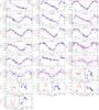 |
Fig. 15 NGC 5286: light curves of the known and new variables discovered in this globular cluster. Symbols are the same as in Fig. 7. |
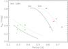 |
Fig. 16 Amplitude-period diagram for the RR Lyrae stars in the globular cluster NGC 5286. |
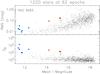 |
Fig. 17 Root mean square (rms) magnitude deviation (top) and SB statistic (bottom) versus the mean I magnitude for the 1220 stars detected in the field of view of the reference image for NGC 6093. Coloured points follow the convention adopted in Table 2 to identify the types of variables found in the field of this globular cluster. |
For the remaining variable stars in the field of view, three of them are RR0 (V10, V19, and V20), one is a RR1 (V17), and V34 is a Nova. Light curves for these stars are presented in Fig. 20. We have improved on the period estimates published by Kopacki (2013) for the four RR Lyrae variables since we observed them using a time baseline of over one year, whereas Kopacki (2013) analysed observations spanning only one week.
V34: this is the Nova discovered by Arthur von Auwers at Koenigsberg Observatory on May 21, 1860 (Luther 1860). As pointed out in the Catalogue of Variable Stars in Galactic Globular Clusters (Clement et al. 2001), an account of its discovery was given by Sawyer (1938) in which a maximum visual apparent magnitude of 6.8 mag was reported using the data taken by von Auwers and Luther. Another review can also be found in Wehlau et al. (1990). However, no observations of the Nova in outburst have been made until the present study. During our 2013 observing campaign, we caught an outburst of amplitude ~0.36 mag starting at around HJD ~ 2 456 500 d which lasted for ~50 days. In our 2014 data the Nova continued at its baseline magnitude at ~16.44 mag.
Dieball et al. (2010) in their ultraviolet survey assigned the label CX01 to an X-ray source that was found to be associated with the position of the Nova at the coordinates RA(J2000) = 16:17:02.817 and Dec(J2000) = −22:58:33.92. These coordinates match with the position of the outburst found in this work and details are given in Table 7.
The position in the colour magnitude diagram shown in Fig. 18 suggests that this system is a cluster member. It is located at the bottom part of the red giant branch. Its position is plotted with a green five pointed star.
As the Nova with its outburst has shown variability, we have assigned the label V34 to this object.
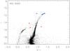 |
Fig. 18 Colour magnitude diagram for the globular cluster NGC 6093 built with V and I magnitudes available in the ACS globular cluster survey extracted from HST images. The variable stars are plotted in colour following the convention adopted in Table 2. |
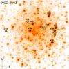 |
Fig. 19 Finding chart for the globular cluster NGC 6093. The image used corresponds to the reference image constructed during the reduction. All known variables and new discoveries are labelled. Image size is ~41 × 41 arcsec2. |
NGC 6656: ephemerides and main characteristics of the variable stars in the field of this globular cluster.
NGC 6681: ephemerides and main characteristics of one variable star in the field of this globular cluster.
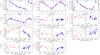 |
Fig. 20 NGC 6093: light curves of the known and new variables discovered in this globular cluster. Symbols are the same as in Fig. 7. |
8.4.2. New variables
A total of six new variables were found in this work. All of them are long-period irregular variables.
V35-V40: these stars are long-period irregular variables. They are located at the top of the red giant branch (see Fig. 18). Their amplitudes go from ~0.04 to 0.13 mag. The star V40 is the one placed on the blue side of the red giant branch. We did not find any kind of regular periodicity in the variation of these stars.
8.5. NGC 6121/C1620-264/M4
This globular cluster was discovered by Philippe Loys de Chéseaux in 17467. This cluster is in the constellation of Scorpius at a distance of 2.2 kpc from the Sun and 5.9 kpc from the Galactic centre. It has a metallicity of [Fe/H] = −1.16 dex and a distance modulus of (m−M)V = 12.82 mag. Its horizontal branch level is at VHB = 13.45 mag.
This globular cluster has approximately 100 known variables in the Catalogue of Variable Stars in Galactic Globular Clusters (Clement et al. 2001) and only three are in the field of view of the reference image; namely V21, V81, and V101. Furthermore, only V21 is bright enough to be detected. The light curve for this RR0 star is shown in Fig. 22. The known period P = 0.4720 d produces a very well phased light curve and is in agreement with the period P = 0.472008 d found in the analysis of this star.
No new variable stars were found in the field covered by the reference image for this globular cluster.
8.6. NGC 6541/C1804-437
This globular cluster was discovered by N. Cacciatore in 18268. It is in the constellation of Corona Australis at 7.5 kpc from the Sun and 2.1 kpc from the Galactic centre. The cluster has a metallicity of [Fe/H] = −1.81 dex, a distance modulus of (m−M)V = 14.82 mag and the level of the horizontal branch is at VHB = 15.35 mag. A total of 843 light curves were extracted in this globular cluster. Most of them have 42 epochs. rms diagram and SB statistic are shown in Fig. 23.
8.6.1. Known variables
This globular cluster has 20 known variables. Four of them are in the field of view of our reference image: V12, V14, V15, and V17. Fiorentino et al. (2014) discovered and classified these stars as SX Phoenicis in their study carried out using observations with the HST. We were only able to recover V14 in our data around 2 arcsec in declination from the reported position for this star in Fiorentino et al. (2014). We did not detect variability at the positions given for V12, V15, and V17 or in their surrounding areas, probably because the stars are too faint to be detected in our reference image. A reference image with higher S/N might be needed in future studies of this globular cluster and longer exposure times for each observation.
V14: for this star we refined the period estimate to 0.064669 d from the previously listed value of 0.0649 d in Fiorentino et al. (2014).
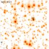 |
Fig. 21 Finding chart for the globular cluster NGC 6121. The image used corresponds to the reference image constructed during the reduction. The only known variable in the field is labelled. Image size is ~41 × 41 arcsec2. |
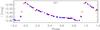 |
Fig. 22 NGC 6121: light curve of the variable V21 in this globular cluster. Symbols are the same as in Fig. 7. |
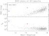 |
Fig. 23 Root mean square (rms) magnitude deviation (top) and SB statistic (bottom) versus the mean I magnitude for the 843 stars detected in the field of view of the reference image for NGC 6541. Coloured points follow the convention adopted in Table 2 to identify the types of variables found in the field of this globular cluster. |
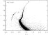 |
Fig. 24 Colour magnitude diagram for the globular cluster NGC 6541 built with V and I magnitudes available in the ACS globular cluster survey extracted from HST images. The variable stars are plotted in colour following the convention adopted in Table 2. |
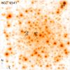 |
Fig. 25 Finding chart for the globular cluster NGC 6541. The image used corresponds to the reference image constructed during the reduction. All known variables and new discoveries are labelled. Image size is ~41 × 41 arcsec2. |
8.6.2. New variables
A total of two new variable stars were found in this globular cluster: one RR Lyrae and one long-period irregular variable.
V21: this star is a RR Lyrae pulsating in the fundamental mode. In the colour–magnitude diagram (Fig. 24) for this cluster it falls exactly in the instability strip of the horizontal branch. It is next to a brighter star (~1.039 arcsec) and this may be why it was not discovered before.
V22: this star is at the top of the red giant branch in the colour–magnitude diagram of the globular cluster (Fig. 24). From the light curve obtained it was possible to measure an amplitude of Ai′ + z′ = 0.17 mag. We classified this star as a long-period irregular variable as it was not possible to find a period.
8.7. NGC 6656/C1833-239/M 22
This globular cluster was discovered by Abraham Ihle in 16659. It is in the constellation of Sagittarius at 3.2 kpc from the Sun and 4.9 kpc from the Galactic centre. The cluster has a metallicity of [Fe/H] = −1.70 dex, a distance modulus of (m−M)V = 13.60 mag and the horizontal branch level is at VHB = 14.15 mag.
8.7.1. Known variables
There are approximately 100 variable sources known for this globular cluster. Only four of these are inside the field of view of the reference image (V35, PK-06, PK-08, and CV1). PK-08 is too faint for us to extract a light curve.
V35: this star is the brightest star in our field of view and it is classified as a semi-regular variable. The star is at the top of the red giant branch in the colour–magnitude diagram shown in Fig. 29. Sahay et al. (2014) found a period of ~56 d. However, we found a period of 141 ± 5 d.
PK-06: this star is classified as an EW eclipsing variable. It was discovered by Pietrukowicz & Kaluzny (2003) and it is their star M22_06. They found a period P = 0.239431 d. However, it does not produce a good phased light curve in our data. In the analysis of this variable, we found a period of P = 0.140851 d which produces a better phased light curve (see Fig. 28). However, our phased light curve is still not as clear as that of Pietrukowicz & Kaluzny (2003).
CV1: the variability of this star was first detected by Sahu et al. (2001) as a suspected microlensing event, but it was not until Anderson et al. (2003) that it was classified as a dwarf nova outburst. The analysis of our light curve for this source shows that it undergoes an outburst of ~3 mag around HJD ~2 456 877, which decays over ~20d. It is in agreement with previous studies. Anderson et al. (2003) found that an earlier outburst lasted ~20−26d with an amplitude of ~3 mag peaking at I ≈ 15 mag. Alonso-Garcia et al. (2015) also observed the 2014 outburst seen in our data and reported a Ks-band brightening of 1 mag. In Fig. 28, we have plotted the light curve for this star.
Our search for new variable sources in this cluster did not yield any.
 |
Fig. 26 NGC 6541: light curves of the known and new variables discovered in this globular cluster. Symbols are the same as in Fig. 7. |
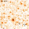 |
Fig. 27 Finding chart for the globular cluster NGC 6656. The image used corresponds to the reference image constructed during the reduction. All known variables and new discoveries are labelled. Image size is ~41 × 41 arcsec2. |
NGC 6723: ephemerides and main characteristics of the variable stars in the field of this globular cluster.
NGC 6752: ephemerides and main characteristics of one variable star in the field of this globular cluster.
 |
Fig. 28 NGC 6656: light curves of the known variables found in this globular cluster. Symbols are the same as in Fig. 7. |
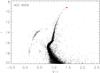 |
Fig. 29 Colour magnitude diagram for the globular cluster NGC 6656 built with V and I magnitudes available in the ACS globular cluster survey extracted from HST images. The variable stars are plotted in colour following the convention adopted in Table 2. |
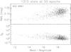 |
Fig. 30 Root mean square (rms) magnitude deviation (top) and SB statistic (bottom) versus the mean I magnitude for the 1315 stars detected in the field of view of the reference image for NGC 6681. The coloured point follows the convention adopted in Table 2 to identify the types of variables found in the field of this globular cluster. |
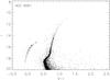 |
Fig. 31 Colour magnitude diagram for the globular cluster NGC 6681 built with V and I magnitudes available in the ACS globular cluster survey extracted from HST images. One variable star is plotted in colour following the convention adopted in Table 2. |
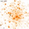 |
Fig. 32 Finding chart for the globular cluster NGC 6681. The image used corresponds to the reference image constructed during the reduction. All known variables and new discoveries are labelled. Image size is ~41 × 41 arcsec2. |
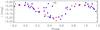 |
Fig. 33 NGC 6681: light curve of the new variable discovered in this globular cluster. Symbols are the same as in Fig. 7. |
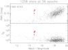 |
Fig. 34 Root mean square (rms) magnitude deviation (top) and SB statistic (bottom) versus the mean I magnitude for the 1258 stars detected in the field of view of the reference image for NGC 6723. Coloured points follow the convention adopted in Table 2 to identify the types of variables found in the field of this globular cluster. |
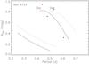 |
Fig. 35 Period-amplitude diagram for the globular cluster NGC 6723. The previously known RR Lyrae are plotted. |
8.8. NGC 6681/C1840-323/M70
This globular cluster was discovered by Charles Messier in 178010. The globular cluster is in the constellation of Sagittarius at 9.0 kpc from the Sun and 2.2 kpc from the Galactic centre. It has a metallicity of [Fe/H] = −1.62 dex, a distance modulus of (m−M)V = 14.99 mag and the horizontal branch level is at VHB = 15.55 mag.
There are a total of 1315 light curves available for this cluster to be analysed. Most of them have 50 epochs. The rms and SB diagrams can be found in Fig. 30. Variable stars studied in this work are plotted in colour.
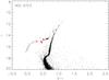 |
Fig. 36 Colour magnitude diagram for the globular cluster NGC 6723 built with V and I magnitudes available in the ACS globular cluster survey extracted from HST images. The variable stars are plotted in colour following the convention adopted in Table 2. |
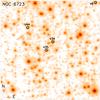 |
Fig. 37 Finding chart for the globular cluster NGC 6723. The image used corresponds to the reference image constructed during the reduction. All known variables and new discoveries are labelled. Image size is ~41 × 41 arcsec2. |
8.8.1. Known variables
This globular cluster has only five known variables, none of which are in the field of view of our reference image.
Kadla et al. (1996) reported several RR Lyrae candidates based on the position of the stars in the instability strip of the horizontal branch but none of them matched the position of the only variable star found in the field of view covered by our reference image, which is the new variable V6 explained in the next section.
8.8.2. New variables
One new RR Lyrae was discovered in this globular cluster.
V6: this star has an amplitude of 0.23 mag and a period of P = 0.341644 d. The star is placed just at the instability strip of the horizontal branch (see Fig. 31). It is clearly a previously unknown RR Lyrae of type RR1. The light curve for this variable is shown in Fig. 33.
8.9. NGC 6723/C1856-367
This globular cluster was discovered by James Dunlop in 182611. It is in the constellation of Sagittarius at a distance of 8.7 kpc from the Sun and 2.6 kpc from the Galactic centre. It has a metallicity of [Fe/H] = −1.10 dex, a distance modulus of (m−M)V = 14.84 mag and the horizontal branch level is at VHB = 15.48 mag.
In Fig. 34, the rms and SB statistic diagrams for 1258 stars in the globular cluster NGC 6723 are shown. Most of the light curves have 56 epochs. Variable stars analysed in this work are plotted in colour following the convention adopted in Table 2.
8.9.1. Known variables
This globular cluster has 47 known variables stars in the Catalogue of Variable Stars in Galactic Globular Clusters (Clement et al. 2001). 43 are classified as RR Lyrae, two as semi-regular variables, one as a T Tauri star that does not seem to be a cluster member and one as a SX Phoenicis. Four of the known RR Lyrae are in the field of our reference frame (V8, V34, V35 and V44). They are RR0 pulsating stars. The star V8 was discovered by Bailey (1902) and although it is close to the reference image border, it was possible to obtain 16 data points. The stars V34, V35, and V44 were discovered by Lee et al. (2014). In the colour magnitude diagram for this globular cluster (see Fig. 36), these variables are placed just in the instability strip of the horizontal branch. Light curves for these variables are shown in Fig. 38.
The four RR Lyrae in the field of our images are plotted in the period-amplitude diagram shown in Fig. 35. It is possible to see that, even though V34 and V35 have the Blazhko effect, all of them are following the model of fundamental mode pulsating stars for Oosterhoff type I, which is consistent with the Oosterhoff classification for this cluster (see Lee et al. 2014, Kovacs et al. 1986, and references therein).
The periods that we derive for the 4 RR Lyrae stars are perfectly consistent with those derived by Lee et al. (2014) using a 10-year baseline. Furthermore, the Blazhko effect in V34 and V35 is also evident in our light curves.
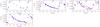 |
Fig. 38 NGC 6723: light curves of the known variables in this globular cluster. Symbols are the same as in Fig. 7. |
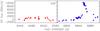 |
Fig. 39 NGC 6752: light curve of the variable V26 in this globular cluster. Symbols are the same as in Fig. 7. We plot the quantity fdiff(t) /p(t) since a reference flux is not available. |
No new variable stars were found in the field covered by the reference image for this globular cluster.
8.10. NGC 6752/C1906-600/C93
This globular cluster was discovered by James Dunlop in 182612. It is in the constellation of Pavo with a distance of 4.0 kpc from the Sun and 5.2 kpc from the Galactic centre. It has a metallicity of [Fe/H] = −1.54 dex, a distance modulus of (m−M)V = 13.13 mag and the level of its horizontal branch is at VHB = 13.70 mag.
8.10.1. Known variables
There are 32 known variable sources in this globular cluster which are listed in the Catalogue of Variable Stars in Galactic Globular Clusters (Clement et al. 2001). Six of them are in the field of view of our reference image. Three are millisecond pulsars (PSRB, PSRD, and PSRE) discovered by D’Amico et al. (2001, 2002). We could not find an optical counterpart in our reference image. Three more are Dwarf Novae (V25, V26, V27) discovered by Thomson et al. (2012) of which V26 is the only object in which we could detect variability.
V26: this star is classified as a dwarf nova. A finding chart for V26 is already available in Thomson et al. (2012). It was not possible to detect this star in the reference image in its quiescent state. However, it was possible to clearly detect one outburst in the difference images. As a result, in Fig. 39 the difference fluxes measured for this star are plotted against their Heliocentric Julian Day. It is possible to see that in the 2013 campaign the star was in its quiescent state. In the 2014 observing season, the outburst started around HJD 2 456 840 with a maximum at HJD ~ 2 456 858.8532 and lasted ~80 d.
We did not find any evidence in our data for new variable stars in this globular cluster.
9. Conclusions
This study shows how the effects of the atmospheric turbulence can be minimized on images taken with ground-based telescopes by using EMCCDs and the “shift-and-add” technique. With this technique was also possible to avoid saturated stars in the field of the globular clusters observed which allowed the discovery of variable stars in the brightest zone of the colour−magnitude diagram such as the top of the red giant branch. The new discoveries are good examples that globular cluster systems still need further studies and are not as well understood as we have thought. A summary of the results obtained in this work are the following:
-
1.
The central regions of ten globular clusters were studied.
-
2.
The benefits of using EMCCDs and the shift-and-add technique were shown.
-
3.
A total of 12 541 stars in the fields covered in the centre of each globular cluster were studied for variable star detection.
-
4.
Light curves for 31 previously known variables are presented (3 L, 2 SR, 20 RR Lyrae, 1 SX Phe, 3 cataclysmic variables, 1 EW, and 1 NC). Period improvement and ephemerides are presented for most of them as well.
-
5.
The discovery of 30 variable stars is presented (16 L, 7 SR, 4 RR Lyrae, 1 SX Phe, and 2 NC). Period and ephemerides calculations were also done.
-
6.
Light curves are available for all variable stars studied in this work.
DanDIA is built from the DanIDL library of IDL routines available at http://www.danidl.co.uk
Acknowledgments
Our thanks go to Christine Clement for clarifying the known variable star content of each cluster and the numbering systems within each one while we were working on these clusters. This support to the astronomical community is very much appreciated. The Danish 1.54m telescope is operated with a grant from the Danish Natural Science Foundation (FNU). R.F.J. thanks Ian Taylor for sorting out all my computational needs on my arrival at St Andrews. RFJ also thanks Katherine White for her comments and suggestions on the improvement of my English language. This publication was made possible by NPRP grant # X-019-1-006 from the Qatar National Research Fund (a member of Qatar Foundation). The statements made herein are solely the responsibility of the authors. K.H. acknowledges support from STFC grant ST/M001296/1. G.D. acknowledges Regione Campania for support from POR-FSE Campania 2014-2020. T.H. is supported by a Sapere Aude Starting Grant from the Danish Council for Independent Research. Research at Centre for Star and Planet Formation is funded by the Danish National Research Foundation. T.C.H. acknowledges support from the Korea Research Council of Fundamental Science & Technology (KRCF) via the KRCF Young Scientist Research Fellowship Programme and for financial support from KASI travel grant number 2013-9-400-00 & 2014-1-400-06. O.W. and J. Surdej acknowledge support from the Communauté française de Belgique – Actions de recherche concertées – Académie Wallonie-Europe. This work has made extensive use of the ADS and SIMBAD services, for which we are thankful.
References
- Alard, C., & Lupton, R. H. 1998, ApJ, 503, 325 [NASA ADS] [CrossRef] [Google Scholar]
- Albrow, M. D., Gilliland, R. L., Brown, T. M., et al. 2001, ApJ, 559, 1060 [NASA ADS] [CrossRef] [Google Scholar]
- Alonso-Garcia, J., Minniti, D., Angeloni, R., et al. 2015, ATel, 7238, 1 [NASA ADS] [Google Scholar]
- Anderson, J., Cool, A. M., & King, I. R. 2003, ApJ, 597, L137 [NASA ADS] [CrossRef] [Google Scholar]
- Anderson, J., Sarajedini, A., Bedin, L. R., et al. 2008, AJ, 135, 2055 [NASA ADS] [CrossRef] [Google Scholar]
- Arellano Ferro, A., Bramich, D. M., Figuera Jaimes, R., Giridhar, S., & Kuppuswamy, K. 2012, MNRAS, 420, 1333 [NASA ADS] [CrossRef] [Google Scholar]
- Bailey, S. I. 1902, Annals of Harvard College Observatory, 38, 1 [Google Scholar]
- Bailey, S. I. 1918, in PAAS, 3, 291 [Google Scholar]
- Barnard, E. E. 1909, ApJ, 29, 72 [NASA ADS] [CrossRef] [Google Scholar]
- Bessell, M. S. 2005, ARA&A, 43, 293 [NASA ADS] [CrossRef] [Google Scholar]
- Bramich, D. M. 2008, MNRAS, 386, L77 [NASA ADS] [CrossRef] [Google Scholar]
- Bramich, D. M., Figuera Jaimes, R., Giridhar, S., & Arellano Ferro, A. 2011, MNRAS, 413, 1275 [NASA ADS] [CrossRef] [Google Scholar]
- Bramich, D. M., Horne, K., Albrow, M. D., et al. 2013, MNRAS, 428, 2275 [NASA ADS] [CrossRef] [Google Scholar]
- Bramich, D. M., Bachelet, E., Alsubai, K. A., Mislis, D., & Parley, N. 2015, A&A, 577, A108 [NASA ADS] [CrossRef] [EDP Sciences] [Google Scholar]
- Clement, C. M., Muzzin, A., Dufton, Q., et al. 2001, AJ, 122, 2587 [NASA ADS] [CrossRef] [Google Scholar]
- D’Amico, N., Lyne, A. G., Manchester, R. N., Possenti, A., & Camilo, F. 2001, ApJ, 548, L171 [NASA ADS] [CrossRef] [Google Scholar]
- D’Amico, N., Possenti, A., Fici, L., et al. 2002, ApJ, 570, L89 [NASA ADS] [CrossRef] [Google Scholar]
- Davis, H. 1917, PASP, 29, 260 [NASA ADS] [CrossRef] [Google Scholar]
- Dieball, A., Long, K. S., Knigge, C., Thomson, G. S., & Zurek, D. R. 2010, ApJ, 710, 332 [NASA ADS] [CrossRef] [Google Scholar]
- Diolaiti, E., Bendinelli, O., Bonaccini, D., et al. 2000, A&AS, 147, 335 [NASA ADS] [CrossRef] [EDP Sciences] [Google Scholar]
- Draper, P. W. 2000, in Astronomical Data Analysis Software and Systems IX, eds. N. Manset, C. Veillet, & D. Crabtree, ASP, 216, 615 [Google Scholar]
- Eddington, A. S. 1916, MNRAS, 76, 572 [NASA ADS] [CrossRef] [Google Scholar]
- Figuera Jaimes, R., Arellano Ferro, A., Bramich, D. M., Giridhar, S., & Kuppuswamy, K. 2013, A&A, 556, A20 [NASA ADS] [CrossRef] [EDP Sciences] [Google Scholar]
- Fiorentino, G., Lanzoni, B., Dalessandro, E., et al. 2014, ApJ, 783, 34 [NASA ADS] [CrossRef] [Google Scholar]
- Freire, P. C., Camilo, F., Lorimer, D. R., et al. 2001, MNRAS, 326, 901 [NASA ADS] [CrossRef] [Google Scholar]
- Harpsøe, K. B. W., Jørgensen, U. G., Andersen, M. I., & Grundahl, F. 2012, A&A, 542, A23 [NASA ADS] [CrossRef] [EDP Sciences] [Google Scholar]
- Harris, W. E. 1996, AJ, 112, 1487 [NASA ADS] [CrossRef] [Google Scholar]
- Herschel, W. 1786, Roy. Soc. London Philos. Trans. Ser. I, 76, 457 [CrossRef] [Google Scholar]
- Hertzsprung, E. 1915, ApJ, 41, 10 [NASA ADS] [CrossRef] [Google Scholar]
- Jerram, P., Pool, P. J., Bell, R., et al. 2001, in Sensors and Camera Systems for Scientific, Industrial, and Digital Photography Applications II, eds. M. M. Blouke, J. Canosa, & N. Sampat, SPIE Conf. Ser., 4306, 178 [Google Scholar]
- Kadla, Z. I., Gerashchenko, A. N., & Malakhova, Y. N. 1996, IBVS, 4414, 1 [NASA ADS] [Google Scholar]
- Kaluzny, J., Olech, A., Thompson, I. B., et al. 2004, A&A, 424, 1101 [NASA ADS] [CrossRef] [EDP Sciences] [Google Scholar]
- Kopacki, G. 2013, Acta Astron., 63, 91 [NASA ADS] [Google Scholar]
- Kovacs, G., Shlosman, I., & Buchler, J. R. 1986, ApJ, 307, 593 [NASA ADS] [CrossRef] [Google Scholar]
- Kunder, A., Stetson, P. B., Catelan, M., Walker, A. R., & Amigo, P. 2013, AJ, 145, 33 [NASA ADS] [CrossRef] [Google Scholar]
- Lafler, J., & Kinman, T. D. 1965, ApJS, 11, 216 [NASA ADS] [CrossRef] [Google Scholar]
- Lebzelter, T., & Wood, P. R. 2005, A&A, 441, 1117 [NASA ADS] [CrossRef] [EDP Sciences] [Google Scholar]
- Lee, J.-W., López-Morales, M., Hong, K., et al. 2014, ApJS, 210, 6 [NASA ADS] [CrossRef] [Google Scholar]
- Luther. 1860, Astronomical news, 53, 293 [NASA ADS] [CrossRef] [Google Scholar]
- Martínez Roger, C., Perez Fournón, I., & Sánchez, F. 1999, Globular clusters, Proceedings (Cambridge University Press) [Google Scholar]
- Messier, C. 1781, Catalogue des Nebuleuses et des amas d’étoiles (Catalog of Nebulae and Star Clusters), Tech. Rep. [Google Scholar]
- Navarrete, C., Contreras Ramos, R., Catelan, M., et al. 2015, A&A, 577, A99 [NASA ADS] [CrossRef] [EDP Sciences] [Google Scholar]
- O’Meara, S. 2002, The Caldwell Objects, Deep-sky companions (Sky Pub.) [Google Scholar]
- Oort, J. H. 1924, Proc. National Academy of Science, 10, 256 [NASA ADS] [CrossRef] [Google Scholar]
- Oosterhoff, P. T. 1938, Bull. Astron. Inst. Netherlands, 8, 273 [NASA ADS] [Google Scholar]
- Pál, A., & Bakos, G. Á. 2006, PASP, 118, 1474 [NASA ADS] [CrossRef] [Google Scholar]
- Pietrukowicz, P., & Kaluzny, J. 2003, Acta Astron., 53, 371 [NASA ADS] [Google Scholar]
- Sahay, A., Lebzelter, T., & Wood, P. R. 2014, PASA, 31, 12 [NASA ADS] [CrossRef] [Google Scholar]
- Sahu, K. C., Casertano, S., Livio, M., et al. 2001, Nature, 411, 1022 [NASA ADS] [CrossRef] [Google Scholar]
- Samus, N. N., Durlevich, O. V., & et al. 2009a, VizieR Online Data Catalog, B/gcvs [Google Scholar]
- Samus, N. N., Kazarovets, E. V., Pastukhova, E. N., Tsvetkova, T. M., & Durlevich, O. V. 2009b, PASP, 121, 1378 [NASA ADS] [CrossRef] [Google Scholar]
- Sawyer, H. B. 1931, Harvard College Observatory Circular, 366, 1 [NASA ADS] [Google Scholar]
- Sawyer, H. B. 1938, Roy. Astron. Soc. Canada, 32, 69 [Google Scholar]
- Shapley, H. 1916, The Observatory, 39, 452 [NASA ADS] [Google Scholar]
- Shara, M. M., Hinkley, S., & Zurek, D. R. 2005, ApJ, 634, 1272 [NASA ADS] [CrossRef] [Google Scholar]
- Sirianni, M., Jee, M. J., Benítez, N., et al. 2005, PASP, 117, 1049 [NASA ADS] [CrossRef] [Google Scholar]
- Skottfelt, J., Bramich, D. M., Figuera Jaimes, R., et al. 2013, A&A, 553, A111 [NASA ADS] [CrossRef] [EDP Sciences] [Google Scholar]
- Skottfelt, J., Bramich, D. M., Figuera Jaimes, R., et al. 2015a, A&A, 573, A103 [NASA ADS] [CrossRef] [EDP Sciences] [Google Scholar]
- Skottfelt, J., Bramich, D. M., Hundertmark, M., et al. 2015b, A&A, 574, A54 [NASA ADS] [CrossRef] [EDP Sciences] [Google Scholar]
- Smith, N., Giltinan, A., O’Connor, A., et al. 2008, in Astrophys. Space Sci. Libr., 351, eds. D. Phelan, O. Ryan, & A. Shearer, 257 [Google Scholar]
- Stetson, P. B. 1987, PASP, 99, 191 [NASA ADS] [CrossRef] [Google Scholar]
- Thomson, G. S., Knigge, C., Dieball, A., et al. 2012, MNRAS, 423, 2901 [NASA ADS] [CrossRef] [Google Scholar]
- Wehlau, A., Butterworth, S., & Hogg, H. S. 1990, AJ, 99, 1159 [NASA ADS] [CrossRef] [Google Scholar]
- Weldrake, D. T. F., Sackett, P. D., Bridges, T. J., & Freeman, K. C. 2004, AJ, 128, 736 [NASA ADS] [CrossRef] [Google Scholar]
- Weldrake, D. T. F., Sackett, P. D., & Bridges, T. J. 2007, AJ, 133, 1447 [NASA ADS] [CrossRef] [Google Scholar]
- Zorotovic, M., Catelan, M., Smith, H. A., et al. 2010, AJ, 139, 357 [NASA ADS] [CrossRef] [Google Scholar]
All Tables
Time-series I photometry for all known and new variables in the field of view covered in each globular cluster.
Convention used in the variable star classification of this work, based on the definitions of the general catalogue of variable stars (Samus et al. 2009a).
NGC 104: ephemerides and main characteristics of the variable stars in the field of this globular cluster.
NGC 5139: ephemerides and main characteristics of the variable stars in the field of this globular cluster.
NGC 5286: ephemerides and main characteristics of the variable stars in the field of this globular cluster.
NGC 6093: ephemerides and main characteristics of the variable stars in the field of this globular cluster.
NGC 6121: ephemerides and main characteristics of one variable star in the field of this globular cluster.
NGC 6656: ephemerides and main characteristics of the variable stars in the field of this globular cluster.
NGC 6681: ephemerides and main characteristics of one variable star in the field of this globular cluster.
NGC 6723: ephemerides and main characteristics of the variable stars in the field of this globular cluster.
NGC 6752: ephemerides and main characteristics of one variable star in the field of this globular cluster.
All Figures
|
Fig. 1 Histograms with the number of observations per night for each globular cluster studied in this work. Panels on the left: plotted data taken during 2013; panels on the right: data taken during 2014. |
| In the text | |
|
Fig. 2 Standard I magnitude taken from the HST observations as a function of the instrumental i′ + z′ magnitude. The red lines are the fits that best match the data and they are described by the equations in the titles of each plot. The correlation coefficient is 0.999 in all cases. |
| In the text | |
|
Fig. 3 Positions of the 157 known globular clusters in the Galaxy are plotted in the Galactic plane system. The 10 globular clusters studied in this work are labelled in red. Green corresponds to the globular clusters studied in Skottfelt et al. (2015a, 2013). |
| In the text | |
|
Fig. 4 Root mean square (rms) magnitude deviation (top) and SB statistic (bottom) versus the mean I magnitude for the 575 stars detected in the field of view of the reference image for NGC 104. Coloured points follow the convention adopted in Table 2 to identify the types of variables found in the field of this globular cluster. |
| In the text | |
|
Fig. 5 Colour magnitude diagram for the globular cluster NGC 104 built with V and I magnitudes available in the ACS globular cluster survey extracted from HST images. The variable stars are plotted in colour following the convention adopted in Table 2. |
| In the text | |
|
Fig. 6 Finding chart for the globular cluster NGC 104. The image used corresponds to the reference image constructed during the reduction. All known variables and new discoveries are labelled. Image size is ~41 × 41 arcsec2. |
| In the text | |
|
Fig. 7 NGC 104: light curves of the known and new variables discovered in this globular cluster. Red triangles correspond to the data obtained during the year 2013 and blue circles correspond to the data obtained during the year 2014. For EM7, we plot the quantity fdiff(t) /p(t) since a reference flux is not available. |
| In the text | |
|
Fig. 8 Root mean square (rms) magnitude deviation (top) and SB statistic (bottom) versus the mean I magnitude for the 2616 stars detected in the field of view of the reference image for NGC 5139. Coloured points follow the convention adopted in Table 2 to identify the types of variables found in the field of this globular cluster. |
| In the text | |
|
Fig. 9 Colour magnitude diagram of the globular cluster NGC 5139 built with V and I magnitudes available in the ACS globular cluster survey extracted from HST images. The variable stars are plotted in colour following the convention adopted in Table 2. |
| In the text | |
|
Fig. 10 Finding chart for the globular cluster NGC 5139. The image used corresponds to the reference image constructed during the reduction. The new variables discovered are labelled. Image size is ~41 × 41 arcsec2. |
| In the text | |
|
Fig. 11 NGC 5139: light curves of the three new variables discovered in this globular cluster. Symbols are the same as in Fig. 7. |
| In the text | |
|
Fig. 12 Root mean square (rms) magnitude deviation (top) and SB statistic (bottom) versus the mean I magnitude for the 1903 stars detected in the field of view of the reference image for NGC 5286. Coloured points follow the convention adopted in Table 2 to identify the types of variables found in the field of this globular cluster. |
| In the text | |
|
Fig. 13 Colour magnitude diagram for the globular cluster NGC 5286 built with V and I magnitudes available in the ACS globular cluster survey extracted from HST images. The variable stars are plotted in colour following the convention adopted in Table 2. |
| In the text | |
|
Fig. 14 Finding chart for the globular cluster NGC 5286. The image used corresponds to the reference image constructed during the reduction. All known variables and new discoveries are labelled. Image size is ~41 × 41 arcsec2. The image stamps are of size ~4.6 × 4.6 arcsec2. |
| In the text | |
|
Fig. 15 NGC 5286: light curves of the known and new variables discovered in this globular cluster. Symbols are the same as in Fig. 7. |
| In the text | |
|
Fig. 16 Amplitude-period diagram for the RR Lyrae stars in the globular cluster NGC 5286. |
| In the text | |
|
Fig. 17 Root mean square (rms) magnitude deviation (top) and SB statistic (bottom) versus the mean I magnitude for the 1220 stars detected in the field of view of the reference image for NGC 6093. Coloured points follow the convention adopted in Table 2 to identify the types of variables found in the field of this globular cluster. |
| In the text | |
|
Fig. 18 Colour magnitude diagram for the globular cluster NGC 6093 built with V and I magnitudes available in the ACS globular cluster survey extracted from HST images. The variable stars are plotted in colour following the convention adopted in Table 2. |
| In the text | |
|
Fig. 19 Finding chart for the globular cluster NGC 6093. The image used corresponds to the reference image constructed during the reduction. All known variables and new discoveries are labelled. Image size is ~41 × 41 arcsec2. |
| In the text | |
|
Fig. 20 NGC 6093: light curves of the known and new variables discovered in this globular cluster. Symbols are the same as in Fig. 7. |
| In the text | |
|
Fig. 21 Finding chart for the globular cluster NGC 6121. The image used corresponds to the reference image constructed during the reduction. The only known variable in the field is labelled. Image size is ~41 × 41 arcsec2. |
| In the text | |
|
Fig. 22 NGC 6121: light curve of the variable V21 in this globular cluster. Symbols are the same as in Fig. 7. |
| In the text | |
|
Fig. 23 Root mean square (rms) magnitude deviation (top) and SB statistic (bottom) versus the mean I magnitude for the 843 stars detected in the field of view of the reference image for NGC 6541. Coloured points follow the convention adopted in Table 2 to identify the types of variables found in the field of this globular cluster. |
| In the text | |
|
Fig. 24 Colour magnitude diagram for the globular cluster NGC 6541 built with V and I magnitudes available in the ACS globular cluster survey extracted from HST images. The variable stars are plotted in colour following the convention adopted in Table 2. |
| In the text | |
|
Fig. 25 Finding chart for the globular cluster NGC 6541. The image used corresponds to the reference image constructed during the reduction. All known variables and new discoveries are labelled. Image size is ~41 × 41 arcsec2. |
| In the text | |
|
Fig. 26 NGC 6541: light curves of the known and new variables discovered in this globular cluster. Symbols are the same as in Fig. 7. |
| In the text | |
|
Fig. 27 Finding chart for the globular cluster NGC 6656. The image used corresponds to the reference image constructed during the reduction. All known variables and new discoveries are labelled. Image size is ~41 × 41 arcsec2. |
| In the text | |
|
Fig. 28 NGC 6656: light curves of the known variables found in this globular cluster. Symbols are the same as in Fig. 7. |
| In the text | |
|
Fig. 29 Colour magnitude diagram for the globular cluster NGC 6656 built with V and I magnitudes available in the ACS globular cluster survey extracted from HST images. The variable stars are plotted in colour following the convention adopted in Table 2. |
| In the text | |
|
Fig. 30 Root mean square (rms) magnitude deviation (top) and SB statistic (bottom) versus the mean I magnitude for the 1315 stars detected in the field of view of the reference image for NGC 6681. The coloured point follows the convention adopted in Table 2 to identify the types of variables found in the field of this globular cluster. |
| In the text | |
|
Fig. 31 Colour magnitude diagram for the globular cluster NGC 6681 built with V and I magnitudes available in the ACS globular cluster survey extracted from HST images. One variable star is plotted in colour following the convention adopted in Table 2. |
| In the text | |
|
Fig. 32 Finding chart for the globular cluster NGC 6681. The image used corresponds to the reference image constructed during the reduction. All known variables and new discoveries are labelled. Image size is ~41 × 41 arcsec2. |
| In the text | |
|
Fig. 33 NGC 6681: light curve of the new variable discovered in this globular cluster. Symbols are the same as in Fig. 7. |
| In the text | |
|
Fig. 34 Root mean square (rms) magnitude deviation (top) and SB statistic (bottom) versus the mean I magnitude for the 1258 stars detected in the field of view of the reference image for NGC 6723. Coloured points follow the convention adopted in Table 2 to identify the types of variables found in the field of this globular cluster. |
| In the text | |
|
Fig. 35 Period-amplitude diagram for the globular cluster NGC 6723. The previously known RR Lyrae are plotted. |
| In the text | |
|
Fig. 36 Colour magnitude diagram for the globular cluster NGC 6723 built with V and I magnitudes available in the ACS globular cluster survey extracted from HST images. The variable stars are plotted in colour following the convention adopted in Table 2. |
| In the text | |
|
Fig. 37 Finding chart for the globular cluster NGC 6723. The image used corresponds to the reference image constructed during the reduction. All known variables and new discoveries are labelled. Image size is ~41 × 41 arcsec2. |
| In the text | |
|
Fig. 38 NGC 6723: light curves of the known variables in this globular cluster. Symbols are the same as in Fig. 7. |
| In the text | |
|
Fig. 39 NGC 6752: light curve of the variable V26 in this globular cluster. Symbols are the same as in Fig. 7. We plot the quantity fdiff(t) /p(t) since a reference flux is not available. |
| In the text | |
Current usage metrics show cumulative count of Article Views (full-text article views including HTML views, PDF and ePub downloads, according to the available data) and Abstracts Views on Vision4Press platform.
Data correspond to usage on the plateform after 2015. The current usage metrics is available 48-96 hours after online publication and is updated daily on week days.
Initial download of the metrics may take a while.