| Issue |
A&A
Volume 587, March 2016
|
|
|---|---|---|
| Article Number | A139 | |
| Number of page(s) | 27 | |
| Section | Interstellar and circumstellar matter | |
| DOI | https://doi.org/10.1051/0004-6361/201527786 | |
| Published online | 03 March 2016 | |
Herschel-HIFI view of mid-IR quiet massive protostellar objects⋆,⋆⋆
1 Univ. Bordeaux, LAB, UMR 5804, 33270 Floirac, France
e-mail: This email address is being protected from spambots. You need JavaScript enabled to view it.
2 CNRS, LAB, UMR 5804, 33270 Floirac, France
3 CONICYT-Universidad de Chile, Camino del Observatorio 1515, Santiago, Chile
4 SRON Netherlands Institute for Space Research, PO Box 800, 9700 AV Groningen, The Netherlands
5 Max-Planck-Institut für Radioastronomie, Auf dem Hügel 69, 53121 Bonn, Germany
6 Leiden Observatory, Leiden University, PO Box 9513, 2300 RA Leiden, The Netherlands
7 Max-Planck Institut für Extraterrestrische Physik, Giessenbachstrasse 1, 85748 Garching, Germany
8 Harvard-Smithsonian Center for Astrophysics, 60 Garden Street, Cambridge, MA 02138, USA
Received: 19 November 2015
Accepted: 14 January 2016
Abstract
Aims. We present Herschel/HIFI observations of 14 water lines in a small sample of Galactic massive protostellar objects: NGC 6334I(N), DR21(OH), IRAS 16272-4837, and IRAS 05358+3543. Using water as a tracer of the structure and kinematics, we individually study each of these objects with the aim to estimate the amount of water around them, but to also to shed light on the high-mass star formation process.
Methods. We analyzed the gas dynamics from the line profiles using Herschel-HIFI observations acquired as part of the WISH key-project of 14 far-IR water lines (H O, H
O, H O, H
O, H O) and several other species. Then through modeling the observations using the RATRAN radiative transfer code, we estimated outflow, infall, turbulent velocities, and molecular abundances and investigated the correlation with the evolutionary status of each source.
Results. The four sources (and the previously studied W43-MM1) have been ordered in terms of evolution based on their spectral energy distribution from youngest to older: 1) NGC 64334I(N); 2) W43-MM1; 3) DR21(OH); 4) IRAS 16272-4837; 5) IRAS 05358+3543. The molecular line profiles exhibit a broad component coming from the shocks along the cavity walls that is associated with the protostars, and an infalling (or expanding, for IRAS 05358+3543) and passively heated envelope component, with highly supersonic turbulence that probably increases with the distance from the center. Accretion rates between 6.3 × 10⁻⁵ and 5.6 × 10⁻⁴M⊙ yr-1 are derived from the infall observed in three of our sources. The outer water abundance is estimated to be at the typical value of a few 10-8, while the inner abundance varies from 1.7 × 10⁻⁶ to 1.4 × 10⁻⁴ with respect to H2 depending on the source.
Conclusions. We confirm that regions of massive star formation are highly turbulent and that the turbulence probably increases in the envelope with the distance to the star. The inner abundances are lower than the expected, 10-4, perhaps because our observed lines do not probe deep enough into the inner envelope or because photodissociation through protostellar UV photons is more efficient than expected. We show that the higher the infall or expansion velocity in the protostellar envelope, the higher the inner abundance. This may indicate that higher infall or expansion velocities generate shocks that will sputter water from the ice mantles of dust grains in the inner region. High-velocity water must be formed in the gas phase from shocked material.
Key words: ISM: molecules / ISM: abundances / stars: formation / stars: protostars / stars: early-type / line: profiles
Herschel is an ESA space observatory with science instruments provided by European-led Principal Investigator consortia and with important participation from NASA.
The reduced HIFI data are only available at the CDS via anonymous ftp to cdsarc.u-strasbg.fr (130.79.128.5) or via http://cdsarc.u-strasbg.fr/viz-bin/qcat?J/A+A/587/A139
© ESO, 2016
1. Introduction
The importance of high-mass stars (M > 8 M⊙) in the matter cycle in the Universe and the evolution of galaxies is well known (e.g., Zinnecker & Yorke 2007; Tan et al. 2014). As powerful sources of UV and driving strong outflows, they deeply influence their environment. Despite this fundamental role, their formation is still not well understood because they are rare, are often located at large distances, and are embedded.
Empirically, high-mass star formation may be divided into several stages (e.g., van der Tak et al. 2000; Beuther et al. 2007; Mottram et al. 2011), which leads to the (not unique) following evolutionary sequence: from the initial stage massive pre-stellar cores (PSCs) to high-mass protostellar objects (HMPOs), hot molecular cores (HMCs), and finally to the more evolved ultra-compact HII regions (UCHII). While pre-stellar cores represent a quiet phase without significant luminosity (Ragan et al. 2012) or activity (infall, outflow, or maser activity, Shipman et al. 2014), the HMPO stage is characterized by the presence of an active protostar exhibiting infall of a massive envelope onto the central star and strong outflows. Then, the temperature of the inner regions of the protostellar envelope will increase, exceeding the evaporation limits of molecules on the grains, hence enriching the envelope with complex molecules leading to the formation of a HMC. Later when the star gets hot enough to emit significant Lyman continuum, it will ionize the surrounding gas, leading to the formation of an UCHII. Based on the definition of Motte et al. (2007), HMPO sources can be divided into two different types depending on their 21 μm flux: the mid-IR-quiet dense (F21 < 10 Jy) and the more evolved mid-IR bright cores (F21 > 10 Jy). The distinction that mid-IR quiet and bright are different evolutionary stages is not obvious since geometry plays a significant role, and this still uncertain scenario may evolve and be constrained, for example, by further observations. We here study mid-IR quiet HMPOs.
The classical question in massive star formation was how the accretion of matter can overcome radiative pressure. This is now well addressed by models considering a protostar-disk system (e.g., Yorke & Sonnhalter 2002; Krumholz et al. 2005; Banerjee & Pudritz 2007). More recently, the generation simulations of Kuiper et al. (2010, 2015) demonstrated that disk accretion and protostellar outflows enable the accretion process to continue for longer times and then to reach final star masses well above the upper mass limit of spherically symmetric accretion. The two main theoretical scenarios both require the presence of a disk and high accretion rates: (a) a monolithic collapse scenario (Tan & McKee 2002; McKee & Tan 2003), also called turbulent core model; and (b) a highly dynamical competitive accretion model involving the formation of a cluster (Bonnell & Bate 2006). The turbulent core model implies supersonic turbulence in the protostellar envelope, while the competitive accretion model predicts cores that are subsonic, but still embedded in a supersonic envelope (see Krumholz & Bonnell 2009). Moreover, massive star formation triggered by converging turbulent flows is predicted by numerical simulations (e.g., Vázquez-Semadeni et al. 2007; Heitsch et al. 2008) and has been proposed for several objects (e.g., DR21(OH), Csengeri et al. 2011).
Several studies have been conducted on water chemistry in massive protostars, well before the age of IR satellites. Jacq et al. (1990) observed the 313−220 transition of HO at 203 GHz, one of the very few thermal water lines observable from ground, toward several sources, including one we study here, DR21(OH). They concluded that the water abundance is typically on the order of 10-5 (relative to H2) or lower in hot dense regions (where T> 100 K). While in cold regions water is mostly found as ice on dust grains, at temperatures T > 100 K the gas-phase water abundance increases by several orders of magnitudes as the ice evaporates (Fraser et al. 2001; Aikawa et al. 2008). A second increase occurs at T ≥ 250 K, when gas-phase reactions drive all available oxygen into water (e.g., Charnley 1997; van Dishoeck et al. 2013). The launch of ISO and SWAS satellites offered the possibility of observing for the first time ro-vibrational fundamental bands of water in absorption against bright infrared continuum sources. Hence, the inner water abundance has been probed toward AFGL2591 by Helmich et al. (1996) and was estimated to be 2−6 × 10⁻⁵, similar to that of solid H2O (van Dishoeck & Helmich 1996). Some uncertainties remain on the water content because of the low spectral resolution of the ISO data. The outer abundance (in regions where T< 100 K) has been estimated to be 0.8−13 × 10-9 by Snell et al. (2000) using SWAS satellite data (from observations of the 557 GHz water line) in several sources (e.g., AFGL2591). Boonman et al. (2003) later combined ISO-SWS/LWS/SWAS data to derive an abundance profile in a set of massive protostars, including W3IRS5 and AFGL2591. Their preferred scenario is a model with ice evaporation occurring at T ~ 90−110 K in the inner part (χin ~ 10-4) with a low outer water abundance (χout ~ 10-8). This jump-like radial profile for water has been confirmed by van der Tak et al. (2006) using new interferometric observations from the ground of the 203 GHz HO line, and by the results of time-dependent gas-grain chemical modeling by Kaźmierczak-Barthel et al. (2015). Observing the same HO line in younger sources, including two of our sample, Marseille et al. (2010b) have not been able to constrain the inner abundance, but have derived a global water abundance of 5 × 10⁻⁸ and 5 × 10⁻⁷, respectively, for the HMPOs W43-MM1 and DR21(OH).
As shown by Chavarría et al. (2010), Herpin et al. (2012), or van der Wiel et al. (2013), from single-dish observations it is only possible to trace the dynamics of gas in the deeply embedded phase of star formation using spectrally resolved emission-line profiles. This has been done before with species like CS by van der Tak et al. (2000) and Shirley et al. (2003). Infall motion and supersonic turbulence in massive dense clouds have been further studied in HCN and CS surveys by Wu et al. (2010), or using HCO+ and N2H+ by Schlingman et al. (2011). In addition, spectroscopic observations of the molecular content of the gas surrounding the protostellar object shed light on the complex chemistry occurring in these environments (e.g., Herpin et al. 2009; Benz et al. 2010; Bruderer et al. 2010; Wyrowski et al. 2010). Within the CHESS Herschel program (Ceccarelli et al. 2010), the HIFI spectral survey of AFGL2591 has been performed, and the chemical structure of its protostellar envelope has been modeled by Kaźmierczak-Barthel et al. (2015). More generally, understanding the chemical evolution of HM protostars is now a very active field: for instance, Gerner et al. (2014) have shown that the chemical composition evolves along with the evolutionary stages.
Source list and parameters.
Probing star formation using spectroscopic observations of water was the main goal of the guaranteed-time key program Water In Star-forming regions with Herschel (WISH, van Dishoeck et al. 2011). Water was indeed one of the main drivers of the Herschel Space Observatory mission (hereafter Herschel, Pilbratt et al. 2010) and particularly of the HIFI spectroscopy instrument (de Graauw et al. 2010). The WISH program aims at characterizing the dynamics of the different components of the gas surrounding the central massive core and intends to measure the amount of cooling that water lines provide.
A sample of 19 massive protostars, covering all phases of high-mass star formation, has been observed within WISH. In addition, four pre-stellar cores have been studied by Shipman et al. (2014). The velocity profiles of the low-excitation H2O lines toward this sample have been presented by van der Tak et al. (2013), without detailed modeling. They decomposed HIFI water line spectra into three distinct physical components: (i) dense cores (protostellar envelopes) usually seen as medium or narrow absorption or emission; (ii) outflows seen as broader features; and (iii) absorptions by foreground clouds along the line of sight. More generally, the line profiles obtained in low- (Kristensen et al. 2010), intermediate- (Johnstone et al. 2010), and high-mass (see W3IRS5, Chavarría et al. 2010) young stellar objects exhibit similar velocity components (San José-García et al. 2013; Mottram et al. 2014): a broad (full width at half maximum, FWHM ~ 25 kms-1), a medium (~5−10 kms-1), and a narrower component (<5 kms-1).
We here focus on the analysis of the water observations toward the mid-IR quiet massive protostars of the WISH sample. A similar study has been conducted by Choi et al. (in prep.) for mid-IR bright sources. Using the high-velocity resolution of the HIFI instrument, we study the dynamics of the gas, estimate the infall and turbulent velocities present in the protostellar envelopes, and derive the H2O abundances in these sources. Sections 2 and 3 present our observations and source sample. Results coming from Gaussian (water and other species) line fittings are given in Sect. 4, while a detailed line analysis is given in Sect. 5. We then model the observations using a radiative transfer code in Sect. 6. We estimate the outflow and infall velocities, turbulent velocity, molecular abundances, and the physical structure of the sources. We finally discuss (Sect. 7) the results in terms of massive-star formation scenarios and compare them to previous studies, in particular to Herpin et al. (2012).
Herschel/HIFI observed water line transitions in the source sample.
2. Observations
Fourteen water lines (see Table 2) have been observed with HIFI at frequencies between 547 and 1670 GHz toward the whole source sample in 2010 and 2011 (list of observation identification numbers, obsids, are given in Appendix A.1). An additional high-energy water line at 970.3150 GHz has been observed toward DR21(OH). The observations are part of the WISH GT-KP.
Data were taken simultaneously in H and V polarizations using both the acousto-optical Wide-Band Spectrometer (WBS) with 1.1 MHz resolution and the digital auto-correlator or High-Resolution Spectrometer (HRS) that provides higher spectral resolution (125 kHz). We used the double beam- switch observing mode with a throw of 3′. The off positions were inspected and do not show any H2O or significant continuum emission. The frequencies, energy of the upper levels, system temperatures, integration times and rms noise level at a given spectral resolution for each of the lines are provided in Table 2. Calibration of the raw data into the TA scale was performed by the in-orbit system (Roelfsema et al. 2012); conversion to Tmb was made using the latest beam efficiency estimate from October 20141 given in Table 2 and a forward efficiency of 0.96. HIFI receivers are double-sideband with a sideband ratio close to unity (Roelfsema et al. 2012). The flux scale accuracy is estimated to be around 10% for bands 1 and 2, 15% for bands 3 and 4, and 20% in bands 6 and 71. The frequency calibration accuracy is 20 kHz and 100 kHz (i.e., better than 0.06 kms-1) for HRS and WBS observations, respectively. Data calibration was performed in the Herschel Interactive Processing Environment (HIPE, Ott 2010) version 12.1. Further analyses such as a Gaussian fit was made within the CLASS2 package. These lines are not expected to be polarized, therefore data from the two polarizations were averaged together after inspection. For all observations, we checked for possible contamination from lines in the image sideband of the receiver, but found none. Because HIFI is operating in double-sideband, the measured continuum level has been divided by a factor of 2 (in the figures and tables) to be directly compared to the single-sideband line profiles (this is justified because the sideband gain ratio is close to 1).
3. Source sample
Five sources are studied here: NGC 6334I(N), DR21(OH), IRAS 16272-4837, and IRAS 05358+3543. We analyzed their entire water observations set for the first time here, but results for W43-MM1 results have been presented in Herpin et al. (2012). The source coordinates, luminosity, distance, and velocities are given in Table 1. The position observed corresponds to the peak of the mm continuum emission from the literature (see van der Tak et al. 2013). The selected sources are mid-IR-quiet dense cores (Motte et al. 2007), with bolometric luminosities 0.19−2.4 × 10⁴L⊙ at distances 1.7–5.5 kpc and sizes (radius) in mm continuum of ~0.26–0.82 pc (see Appendix C in van der Tak et al. 2013), hence larger than a 20″ beam (0.15−0.55 pc at these distances). Even if these massive dense cores are expected to be fragmented on small scales, only a small fraction of the total mass is in individual fragments, except for the dominant central source (see references in the following for each source). As a consequence, the large-scale, average-density profile of the cores applies well down to the smallest structures observable with HIFI.
The source NGC 6334 I(N), located in the northern part of the filament in the central region of NGC 6334, has been extensively studied at mm/submm wavelengths (e.g., Hunter et al. 2006, 2014). Brogan et al. (2009) imaged NGC 6334 I(N) at ~2″ angular resolution using the SMA. They detected a cluster of compact sources, SMA1-SMA7 (most of them within the HIFI beams), in the 1.3 mm dust continuum emission, with gas masses of 6−74 M⊙. Spectral line data show evidence of infall accelerating with depth into SMA1 and multiple outflows. We note that parameters for this source and NGC 6334I were confused in van Dishoeck et al. (2011). Observation with HIFI of NGC 6334I have been presented by Emprechtinger et al. (2013).
DR21(OH) is located in the Cygnus X region, in the dense DR 21 filamentary ridge, where active star formation and global infall motions are observed (Csengeri et al. 2011; Hennemann et al. 2012). Infall signatures in DR21(OH) are observed in low-J CS lines on the same spatial scale as is covered by our observations (Chandler et al. 1993). Girart et al. (2013) defined this rich molecular source as a highly fragmented, magnetized, and turbulent dense core. The DR21(OH) core is formed by two main dusty condensations, MM 1 and MM 2, split into a cluster of dusty sources at scales of 1000 AU (Zapata et al. 2012). MM1 contains a hot core and shows centimeter continuum emission (Araya et al. 2009). Very active and powerful outflows are detected.
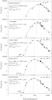 |
Fig. 1 Spectral energy distributions obtained from the 1D model overlaid on observed flux densities of each source. Peak flux densities in the millimeter range have been adjusted to fit the radial extent of the model. Each caption gives the temperatures of the black body components (top right), the maximum flux Fmax, and the corresponding wavelength of the SED, the flux F12 at 12 μm, and the contribution of the hot part (F35, integrated flux for λ< 35 μm) to the total integrated flux Ftotal (top left). |
In contrast, less information is available about the more luminous (L ~ 2.4 × 10⁴L⊙ ) source IRAS 16272-4837. From MSX observations and studies by Garay et al. (2007), this source can unambiguously be classified as a massive star-forming region in a very early evolutionary stage, a mid-IR-quiet HMPO (F21 = 2.2 Jy). No radio continuum emission was detected. The 1.2 mm emission arises from a central component surrounded by more extended gas (region of 41″ × 25″, Faúndez et al. 2004), and the line profiles observed suggest that the molecular gas is undergoing infalling motions.
IRAS 05358+3543 is a relatively low-luminosity (L ~ 6.3 × 10³L⊙ ) and nearby (1.8 kpc) massive dense core, composed of four main sources, all within a box of 4′′× 6′′ (Leurini et al. 2007; Palau et al. 2014), hence within the Herschel telescope beam at all frequencies. Two of these sources are part of a protobinary system with a dynamical age of ~3.6 × 10⁴ yr (Beuther et al. 2007). Several molecular outflows are observed (Beuther et al. 2002a), but no infall is detected (Herpin et al. 2009). The integrated gas mass is estimated to 142 M⊙ by van der Tak et al. (2013). Leurini et al. (2007) suggested that the main source mm1a harbors a hot core with T ~ 220(75 <T< 330) K and may contain a massive circumstellar disk. Because of its 21-micron flux density (11.9 Jy), this source is in between the mid-IR-quiet and mid-IR-bright HMPO stages.
Continuum emission from our sources is determined with well-sampled observations from various telescopes including IRAS (archive3), Spitzer (archive4), MSX (archive5), JCMT (archive6, and Vallée & Fiege 2006; Sandell 2000; McCutcheon et al. 2000), KAO (Harvey et al. 1986; Lester et al. 1985), CSO (Motte et al. 2003), SMA (Beuther et al. 2007; Hunter et al. 2006), APEX, SEST (Garay et al. 2007; Muñoz et al. 2007), IRAM-30m (Beuther et al. 2002b; Motte et al. 2007), IRAM-PdB (Beuther et al. 2007), VLA (Beuther et al. 2002a; Rodríguez et al. 2007), ATCA (Walsh et al. 1998; Beuther et al. 2008), OVRO (Woody et al. 1989), and Herschel-HIFI/PACS (van der Tak et al. 2013). In particular, flux densities below 35 μm come from Spitzer and MSX observations. Hence, the spectral energy distribution (SED) for these sources is particularly well constrained. Following the method of Herpin et al. (2009), we propose a rough evolutionary classification of our five objects from the fitted SEDs shown in Fig. 1 (the reference spatial resolution is the beam of the observation at 1.1 or 1.2 mm, i.e., 11′′ with IRAM-30 m for IRAS 05358, W43MM1, and DR21(OH), and 24′′ with JCMT or SEST for the two other sources), using the following parameters:
-
flux density at 12 μm,
-
flux density at 21 μm,
-
wavelength and flux density of the maximum continuum emission,
-
contribution of the hot part (λ< 35 μm) to the total integrated flux.
In addition, we also use the evolutionary tracer  first introduced by Bontemps et al. (1996) for low-mass objects: this quantity increases with the evolutionary status of the source. It is assumed that less evolved sources are colder, hence the SED peaks at longer wavelength with weaker flux. As the massive core evolves, it becomes warmer, thereby heating the dust. As a consequence, the contribution of the flux at shorter wavelength (F35, the integrated flux density for λ< 35 μm) increases.
Comparison of these quantities (Table 1) leads to the following evolutionary sequence that extends from youngest to older: 1) NGC 64334I(N); 2) W43-MM1; 3) DR21(OH); 4) IRAS 16272-4837; 5) IRAS 05358+3543. The fact that three different estimates give the same order lends credibility to this sequence. We adopt this sequence for the following discussion. Nevertheless, we note that the order of DR21(OH) and IRAS 16272-4837 can be inverted if the criterion is used alone (see values in Table 1) or if we consider that DR21(OH) harbors a hot core like IRAS 05358.
4. Results
The spectra including continuum emission are presented in Figs. 2−5 for the rare isotopologs (HO, HO) and HO for all sources, except W43-MM1, which was presented in Herpin et al. (2012). Spectra of the H2O 111−000 (and HO), 202−111, and 212−101 lines have also been included in van der Tak et al. (2013). In addition, Figs. B.1−B.3 in Appendix B display lines from other species than water that are serendipitously covered in our data. In most cases, we show the HRS spectra, except for the ground-state p-HO 111−000, p-H2O 111−000, and o-H2O 212−101 lines, where WBS spectra were used since the velocity range covered by the HRS was insufficient to show the broad component. In a few cases (e.g., o-H2O 212−101 spectra in NGC 6334I(N)), the detected absorption is slightly below the continuum, but still within the flux uncertainties (see Sect. 2).
Several foreground clouds (van der Tak et al. 2013) contribute to the spectra in NGC 6334I(N), DR21(OH) and IRAS 16272 in terms of water absorption at Vlsr shifted with respect to source velocity in the o-H2O 110−101, p-H2O 111−000 and o-H2O 212−101 lines spectra (absorption is also visible in the o-H2O 221−212 spectra in DR21(OH)). These foreground clouds are not analyzed here.
4.1. Velocity components
For each transition, we derived the peak, or minimum (in case of absorption), main-beam and continuum temperatures, the full width at zero intensity (FWZI, see Mottram et al. 2014, for details), half-power line widths for the different line components from multi-component Gaussian fits, and opacities for lines in absorption. Line parameters are given in Tables 3−6. An example of the Gaussian fits is given for IRAS 05358 in Appendix C. Our results are consistent with van der Tak et al. (2013) and San Jose-Garcia et al. (2016) and do not depend on the adopted method.
We follow the terminology adopted in previous WISH papers (e.g., Johnstone et al. 2010; Kristensen et al. 2010; Herpin et al. 2012): narrow (<5 kms-1), medium (FWHM ≃ 5−10 kms-1), and broad (FWHM ≃ 20−35 kms-1). The narrow component centered at the source velocity is characterized by small FWHM and offset velocity, and is called envelope component, that is, emission from the quiescent envelope, the signature of the passively heated envelope. Both broad and medium components arise in cavity shocks, which are shocks along the cavity walls according to the model of Mottram et al. (2014). The medium component is a narrower version of the broad component (also called narrow outflow by van der Tak et al. 2013), coming from a thin layer (1−30 AU) along the outflow cavity where non-dissociative shocks occur. A different physical component, called the medium offset component, with a velocity offset of at least a few km s-1, is observed in low-mass objects and is associated with spot shocks, which are dissociative shocks in the jet itself or at the base of the outflow (Mottram et al. 2014). This component is seen in the HM data by van der Tak et al. (2013) as a narrow outflow in absorption in the 1113 and 1669 GHz water lines and is slightly offset from the envelope velocity.
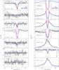 |
Fig. 2 HIFI spectra of H |
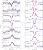 |
Fig. 3 As in Fig. 2, but for DR21(OH) (Vinf = −1.5 and Vturb = 2.5 kms-1 for the constant model). The p-H2O 524−431 line is blended with the CH3OH line at 957.995737 GHz from the LSB. |
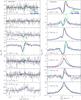 |
Fig. 5 As in Fig. 2, but for IRAS 05358 (Vinf = + 3.0 and Vturb = 2.0 kms-1 for the constant model), more (in green) a varying outer abundance model (see Sect. 6.3) |
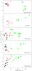 |
Fig. 6 FWHM versus offset of the peak from the source velocity for the Gaussian velocity components found in the water (H |
4.2. Water lines
4.2.1. Rare isotopologs
The more evolved objects, IRAS 05358 and IRAS 16272, exhibit fewer and weaker rare isotopolog lines, with no HO detection. This is not due to a lower source luminosity or a larger distance, as can be inferred from Table 1: IRAS 16272-4837, for instance, exhibits a luminosity similar to that of W43-MM1 and is closer to us. The para ground-state line p-HO 111−000 is detected, as well as the o-HO 312−303 in IRAS 05358, but the o-HO 110−101 line is not detected in IRAS 16272 and IRAS 05358. The fact that no HO and no o-HO 110−101 line are detected in IRAS 16272 and IRAS 05358 is probably due to lower water column densities, hence an insufficient signal-to-noise ratio (S/N).
On the other hand, HO lines are detected in the two other objects. The strongest HO and HO lines are found in DR21(OH). In this source, all observed rare isotopolog lines are detected.
The p-HO 111−000, o-HO 212−101, and p-HO 111−000 lines appear in absorption, and broad signatures from the cavity shocks (red component in emission while the blue one is absorbed) are observed for DR21(OH) and NGC 6334I(N). The o-HO 110−101 line is in absorption for NGC 6334I(N), while it is a blend of absorption (at line center) and emission in DR21(OH). The two other detected HO lines, 202−111 and 312−303, arising from more excited energy levels, are in emission.
Most of the HO/HO line profiles for all sources but W43-MM1 exhibit an envelope component in absorption. We interpret this absorption as resulting from cold material in front of the passively heated envelope. A medium component is detected in several lines as well.
4.2.2. H O
O
All HO lines listed in Table 2 are detected toward all four sources, and the global shape of the line profile for each line is similar from source to source (including W43-MM1): ground-state lines are deeply absorbed, and all lines (except p-H2O 524−431) exhibit a broad component (blue component in absorption for NGC 6334IN). In addition, line profiles consist of a narrow or medium component depending on the source and the line. The p-H2O 202−111 and p-H2O 211−202 lines are asymmetric (see Sect. 5.3) as a result of the infall or expansion of the gas. The o-H2O 221−212 line is in absorption except for IRAS 05358, for which some emission is present as well. The o-H2O 312−303 line is dominated by the broad and medium components in emission.
For the only source in which the p-H2O 524−431 line has been observed, DR21(OH), a medium component, slightly redshifted (by 1.7 kms-1), is observed in emission, but it is blended with a methanol line from the lower sideband at 957.995737 GHz.
Broad, medium, and narrow velocity components are detected in all sources. We observe for the envelope component a similar mean FWHM value of 3 kms-1 for IRAS 16272 (± 0.5) and NGC 6334I(N) (± 0.1), 3.5(± 1.3) kms-1 for IRAS 05358, and 3.8(± 0.7) kms-1 for DR21(OH). The width of the medium component is clearly larger for the less evolved sources (7.1 ± 1.5, 8 ± 2, and 8.0 ± 1.8 kms-1 for NGC 6334IN, W43-MM1, and DR21(OH), respectively) than for IRAS 16272 (5.7 ± 1.3 kms-1) and IRAS 05358 (5.7 ± 0.5 kms-1). The FWHM of the broad component decreases from more than 25 kms-1 for NGC 6334I(N) and W43-MM1 to roughly 20 kms-1 for the three other objects. Figure 6 shows that no or only a small velocity offset is observed for different components: only IRAS 05358 and W43-MM1 exhibit an offset increasing with FWHM (see Sect. 5.1 for a trend analysis).
4.3. Other species
Several other species have been detected toward all sources within the 4 GHz wide WBS spectra (see Tables B.1−B.5): CH3OH, 13CO (J = 5−4 and 10−9), C18O (J = 9−8), CS (11−10), and H2S (30,3−21,2). These lines are detected in all sources in emission.
In addition to the bulk of methanol lines with Eu ≤ 200 K observed in the entire sample, lines involving upper energy levels up to 291, 434, and 514 K are detected in NGC 6334I(N), W43-MM1/IRAS 16272, and DR21(OH), respectively. These lines exhibit an envelope and/or a medium component (and for one or two lines a broad component), similar to what is observed for water lines.
Both detected 13CO J = 5−4 and 10−9 lines exhibit similar profiles, even if the 5−4 line in DR21(OH) is much more self-absorbed at the center because of higher opacity. In addition to the C18O J = 9−8 line, the C18O J = 10−9 transition has been detected toward all sources but IRAS 16272. For each species we note that the line widths are similar for the two observed transitions, and the velocity components derived from the Gaussian fitting are consistent with San José-García et al. (2013; even if our narrow and medium components are only one single component for them in a few cases as they only distinguish between FWHM smaller or larger than 7.5 kms-1).
The water cation H2O+ (111−000, J = 3 / 2−1 / 2) is detected in absorption in all sources, except for NGC 6334I(N): its velocity components indicate that it probably originates from the envelope or outflow for IRAS 05358 and W43-MM1 (see also Benz et al. 2010; Wyrowski et al. 2010, for other high-mass sources), while for DR21(OH) and IRAS 16272 the absorption is redshifted by 5−10 kms-1 and then very likely associated with the foreground clouds described before. In addition, the H3O+ cation is detected in absorption in W43-MM1, but is weaker than the H2O+ line, which, as stressed by Wyrowski et al. (2010), is unexpected.
More species are detected toward the three less evolved sources: deuterated water (HDO) and methyl formate (CH3OCHO), for instance (see Appendix B). But more generally, DR21(OH) is the richest source with twice as many lines detected: the rare isotopolog 13CS, many more methanol lines, dimethyl ether (CH3OCH3), CH+ and OH+ in absorption, H2CO, 34SO, OS18O, and many lines of SO2.
All these lines peak at a mean velocity of VLSR = −15.9 ± 0.3, 46.5 ± 1.9, −3.3 ± 0.8, −4.0 ± 0.6, and 98.4 ± 1.2 kms-1 for IRAS 05358, IRAS 16272, DR21(OH), NGC 6334I(N), and W43-MM1, respectively, which means that they are similar to the source velocity, except for IRAS 05358, whose lines are slightly redshifted.
5. Analysis
5.1. Kinematics
We searched for a correlation for each source between the FWHM and the velocity of the peak of various water components (see Fig. 6). Such a correlation (both increasing together) has been found by Mottram et al. (2014) for Class 0 and I low-mass protostars. A general correlation is observed for IRAS 05358 and W43-MM1: the velocity offset of each component increases with FWHM, hence the broad component is progressively redshifted as the FWHM increases. This could mean that for outflows we see stronger red lobes (Tex higher in the inner part) than blue lobes (where we see the outer part with lower Tex). This trend is seen within the set of envelope and broad components for IRAS 05358, but it is only clear for the broad component in W43-MM1. For IRAS 16272, a correlation is observed for the broad component while nothing is seen for DR21(OH). NGC 6334I(N) tends to show a decrease of Vpeak−Vsource with FWHM. Surprisingly, the broad component tends to be blueshifted with respect to the two other velocity categories. Regardless of the source, no clear trend is seen for the medium component.
This shows that for W43-MM1 and IRAS 05358 the different components globally lie in different regions of the FWHM vs. offset parameter space. We can therefore conclude that these components are formed under different conditions. Obviously, the same conclusion applies to the broad and narrow or medium components for NGC 6334I(N) and perhaps for IRAS 16272. No significant trend is observed for DR21(OH), however.
5.2. Outflow
We used RADEX (van der Tak et al. 2007) to roughly estimate the column density of the H2O in the outflow component for each source, assuming an isothermal homogenous material, shielding envelope emission. Following van der Tak et al. (2010) and Herpin et al. (2012), we adopted n(H2) = 3 × 104 cm-3 and Tkin = 200 K, but also tested neighboring values. The water column density necessary to retrieve the observed intensities and reproduce the observed line ratios for the broad component as derived from the Gaussian fitting (see Sect. 4.1 and Tables 3−6) is 1017,1.2 × 1017,4 × 1016, and 8 × 1016 cm-2 for NGC 6334I(N), DR21(OH) (with Tkin = 300 K for this source), IRAS 16272, and IRAS 05358, respectively. These values are not sensitive to variations by less than 25% of Tkin. In Sect. 7.2 the formation of water in the outflow is studied.
Observed line emission parameters for the detected lines toward NGC 6334I(N).
Observed line emission parameters for the detected lines toward DR21(OH).
Observed line emission parameters for the detected lines toward IRAS 16272.
Observed line emission parameters for the detected water lines toward IRAS 05358.
HO integrated line intensity ratios (not corrected for different beam sizes) for all sources for the broad velocity component.
5.3. Line asymmetries
Compared to optically thin lines (e.g. C18O 9−8 and 13CO 10−9 in most cases), most of the water-line profiles observed in our sources show clear asymmetries, which reveals gas motions. Outflows, infall, and rotation can produce very specific line profiles with characteristic signatures (see Fuller et al. 2005, and references therein).
For all sources but IRAS 05358, blue asymmetric (optically thick) lines, that is, inverse P-Cygni profiles, are observed, which very probably indicates infalling material. In some circumstances, outflow or rotation could also produce a blue asymmetric line profile along a particular line of sight to the source. In IRAS 05358 all lines but p-H2O 211−202 and o-H2O 312−303 have stronger redshifted than blueshifted emission (see Sect. 5.1) with a strong self-absorption dip at the source velocity, or in other words, they show a P-Cygni profile that is typical of expansion.
For IRAS 16272, only the p-H2O 202−111 line exhibits this asymmetry, the other lines are either not optically thick enough or are contaminated by foreground clouds (for ground-state lines). Toward DR21(OH), an inverse P-Cygni profile is observed that is pronounced for the p-H2O 211−202 and p-H2O 202−111 lines and weak for o-H2O 312−303, whose almost symmetric double-horn profile might be produced by the outflow (Fuller et al. 2005). The p-H2O 211−202 and o-H2O 312−303 line profiles, which have a slightly stronger blue than red peak, exhibit a strong self-absorption dip at the source velocity. The HO and HO absorption lines do not show clear asymmetry, but are blueshifted relative to the source velocity, as expected in the case of infall.
The case of NGC 6334I(N) is less clear cut as the absorption of the blue component of the outflow in several lines complicates the interpretation: the infall is only clearly seen in the p-H2O 211−202 line (blue asymmetric profile).
5.4. Opacities and integrated line intensity ratios
Depending on whether the line is in absorption or in emission, two different methods were applied to derive the opacities. For the absorption lines, we estimated the opacities at the maximum of absorption from the line-to-continuum ratio in Tables 3−6 using 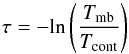 (1)and assuming that the continuum is completely covered by the absorbing layer.
In all sources, even in central regions, all rare isotopolog lines are optically thin (τ< 1). For the three sources (W43-MM1, DR21(OH), and NGC 6334I(N)) that exhibit HO lines, the opacities are similar: 0.11−0.17 and 0.04−0.1 for the 212−101 and 111−000 lines, respectively. These opacities decrease from the less evolved (NGC 6334I(N)) to the more evolved object (DR21(OH)). Interestingly, the HO/HO opacity ratio for the 111−000 line is close to the rare isotopolog ratio (4, see Sect. 6) for W43-MM1, while it is slightly different for the two other objects (2.7 ± 1.1 and 6.2 ± 2.8). Except for IRAS 16272 (τ = 0.06), the opacity of the p-HO 111−000 line is around 0.3 for all sources, higher than what is estimated for the o-HO 110−101 line (0.15−0.20) in W43-MM1 and NGC 6334I(N).
In contrast, all the HO ground-state lines in absorption are optically thick, even totally absorbed for the 1113 and 557 GHz lines. More generally, IRAS 16272 is the source with the lower opacities, while DR21(OH) has the highest opacity. The o-H2O 221−212 line is optically thin in the less evolved sources IRAS 05358 and IRAS 16272.
To study the excitation and physical conditions of the water-emitting gas, we now focus on the opacities of the lines in emission. We first searched for HO/HO line pairs in our sample. Only the 312−303 line exhibits emission for both HO and HO (a blend of emission and absorption prevents us from any accurate comparison of other lines). This is only observed in IRAS 05358, DR21(OH), and NGC 6334I(N). We adopted the following standard abundance ratios (same ratios for all the lines): 4.5 for HO/HO (Thomas & Fuller 2008), and 3 for ortho/para-H2O. Based on Wilson & Rood (1994), the 16O/18O abundance ratio depends on the distance from the Galactic center (while the HO/HO ratio is constant). From the Wilson and Rood results and the distance adopted for IRAS 05358, IRAS 16272, NGC 6334I(N) and DR21(OH) (see Table 1), we derive an HO/HO abundance ratio of 642, 363, 437 and 531, respectively. From the integrated intensity ratios for the 312−303 line, and assuming that both isotopes have the same excitation temperature, we estimate an optical depth on the order of 15−30 for the HO line, the HO line being optically thin (according to our models, see Sect. 6.1).
For sources or components for which HO data are not detected or usable, we followed the method described by Mottram et al. (2014). We used the ratio of the integrated intensity of the different components in pairs of HO lines that share a common level. In Table 7 we compare the ratios obtained for either the medium or broad component of the gas (again we focused on the profiles with obvious components in emission) to the LTE ratios in the optically thin and thick regimes following Goldsmith & Langer (1999), for Tex = 300 K like Mottram et al. (2014; we note that some of the line ratio values in Mottram’s paper are incorrect, and we corrected the ratios from those given in Mottram et al. to the values listed in Table 7), and also for Tex = 100 and 500 K. The thin and thick line ratios for Tex = 300 and 500 K differ by only 10%, which is not significant compared to the observed ratios. Decreasing Tex has a stronger effect, but does not change the interpretation. The line ratios must be corrected by a factor reflecting the different beam sizes of the observations (θ1/θ2, see Table 7). This correction factor is different depending on whether the emission comes from a point source, (θ1/θ2)2, fills the beam in one axis and is point-like in the other, θ1/θ2, or if the emitting region covers both axes (no correction). For our high-mass objects (mainly because of the large distance), we can only assume that the broad component for the ground-state lines covers the beam (based on HIFI maps, see Jacq et al., in prep.) while the other line emission should be smaller than the beam. Hence, we consider the cases θ1/θ2 and (θ1/θ2)2 below. Intermediate cases apply if one line is optically thick but the other is optically thin, or if the transitions are sub-thermally excited at temperatures lower than 300 K.
For the broad component, nearly all line ratios are close to the optically thick limit (after beam correction). IRAS 05358 is a difficult case because the 110−101/ 212−101 ratio is close to the optically thin limit, even considering the large difference in beam size and probable emitting regions. The thick case is probably valid for the 111−000/ 202−111 ratio even if the beam correction factor is close to 1. Nevertheless, considering the high critical densities of these water transitions (see Table 2), these lines can be sub-thermally excited. The medium velocity component in IRAS 05358 is obviously in the optically thick limit, while the conclusion is uncertain for DR21(OH) and IRAS 16272. The LTE conditions may not apply to the medium component in these sources.
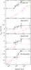 |
Fig. 7 Variation of the turbulent velocity Vturb with the distance R (AU) to the central object as derived from the model for water (in black) and CS (in red, see Appendix D). Error bars illustrate the range of values that has no impact on the model. |
6. Modeling
While the previous sections have presented the different velocity components in the observed line profiles and indications of infall/expansion and outflow in the observed massive protostellar objects, in this section we model the full line profiles in a single spherically symmetric model. The dynamics is driven by turbulence, infalling motions, and outflow components.
6.1. Method
Derived parameters from the RATRAN model and accretion luminosities.
For all sources, the envelope temperature and density structure from van der Tak et al. (2013) were used as input to the 1D-radiative transfer code RATRAN (Hogerheijde & van der Tak 2000) to simultaneously reproduce all the water line profiles, following the method of Herpin et al. (2012). The H2O collisional rate coefficients were taken from Daniel et al. (2011).
As in our previous publications (i.e., Chavarría et al. 2010; Marseille et al. 2010b; Herpin et al. 2012), the source model has two gas components: an outflow and the proto-stellar envelope. The outflow parameters, intensity, and width come from the Gaussian fitting presented in Sect. 4. The envelope contribution is parametrized with three input variables: water abundance (χH2O), turbulent velocity (Vtur), and infall velocity (Vinf). The width of the line is adjusted by varying Vtur. The line asymmetry is reproduced by adjusting the infall velocity parameter. The line intensity is best fitted by adjusting a combination of the abundance, turbulence, and outflow parameters. We adopted the abundance ratios presented in Sect. 5.4. The models assume a jump in the abundance in the inner envelope at 100 K (see Sect. 6.3) due to the evaporation of ice mantles. Table 8 lists the parameters used in the models.
Our modeling strategy was to first fit the rare isotopolog lines (HO and HO) since they are optically thin (see Sect. 5.4). Then we modeled the HO lines starting from the highest energy level (the HO abundances are derived from the HO and HO values times the isotopic abundance ratios). When we were able to reproduce the main features of the profiles by minimizing the residuals (see Herpin et al. 2012) in a grid of values, we modeled the remaining lines using the same parameters, including the outflow component when this was justified.
6.2. Velocity structure
Thanks to the high spectral resolution HIFI observations, we have access to crucial velocity details, as explained in Sect. 4, which help to constrain the source dynamics. In W43-MM1 Herpin et al. (2012) have shown that a turbulence increasing with circumstellar radius provided the best line model. To test this conclusion on the other sample sources, we first tried a model in which the turbulent velocity (and infall or expansion) was constant with radius for all lines, and then a model in which Vturb varied with radius. For the constant model, the best-fit Vturb values (same for all lines) are 2.5, 2.5, 2.2, and 2.0 kms-1 (and Vinf as in Table 8) for DR21(OH), NGC 6334I(N), IRAS 16272, and IRAS 05358, respectively (line models are plotted in red in Figs. 2−5). Except for DR21(OH), the model with constant velocity parameters for all lines fits the HO and HO data quite well, as it does for C18O (San José-García et al. 2013). In contrast, it is not possible to converge to a good model for all HO lines, even though the line profiles of IRAS 05358 and IRAS 16272 are well reproduced.
Inspection of the line profiles (see Tables 3−6) shows that the width of the velocity components is not the same for all lines. As for W43-MM1 (Herpin et al. 2012), we do not expect a model with equal velocity parameters for all lines to fit the data well. Hence, as a second step we tried a model in which the turbulent velocity varied with radius. We tested several possibilities: a power-law variation, then various step profiles based on the turbulent velocity estimated for each line from Tables 3−6. The best models were obtained using the turbulence profiles shown in black in Fig. 7 and overplotted in blue in Figs. 2−5. For IRAS 16272, the adopted turbulent profile is quite flat and improvement of the model fit is small and only significant for the o-H2O 110−101 and p-H2O 202−111 lines. An increasing turbulent velocity in IRAS 05358 gives a better result for at least the p-H2O 211−202 and o-H2O 312−303 lines, the other line profiles being less sensitive to this change. The two other sources, DR21(OH) and NGC 6334I(N), are the most sensitive to the turbulent velocity profile. The relatively steep profiles leading to the best line fit vary from 2 up to at least 3 kms-1 and strongly affect the depth and width of the absorption components (all isotopes). Clearly, a model in which the turbulent velocity increases with radius works better for NGC 6334I(N), DR21(OH), and IRAS 05358, whereas this is less clear for IRAS 16272. Moreover, as explained in Appendix D, this also applies to the CS line modeling (see red plot in Fig. 7).
6.3. Abundance structure
The abundance was constrained by the modeling of the entire set of observed lines. Even if, as underlined by Herpin et al. (2012), only some of these lines (o-HO 312−303 and o-H2O 312−303) are optically thin enough to probe the inner part of the envelope, part of all water line profiles is produced by water excited in the inner part and is revealed by the high spectral resolution of these observations. Moreover, for DR21(OH) we have access to the high-excitation p-H2O 524−431 line. In addition, we applied our model to the HO 313−220 line at 203.3916 GHz (Eup = 204 K) observed toward IRAS 05358 (not detected) and DR21(OH) by Marseille et al. (2010a). As illustrated by the analysis in Visser et al. (2013) for low-mass sources, the 203 GHz line is very useful because it is less optically thick as a result of the lower Einstein A-coefficient, and the dust continuum is more optically thin in the inner envelope, which may certainly affect the high-mass sources. For these reasons, this sample of lines is expected to probe the entire water region.
All line profiles are well reproduced. No deviation from the standard o/p ratio of 3 is found. The HO abundances relative to H2 (see Table 8) range from 1.7 × 10⁻⁶ (IRAS 16272) to 1.3 × 10⁻⁵ (IRAS 05358) in the inner part where T> 100 K, while the outer abundances (where T< 100K) are a few 10-8 (except DR21(OH), 1.4 × 10⁻⁷). These abundances are typical of those found in HMPOs (e.g., Marseille et al. 2010b; Herpin et al. 2012). While the water outer abundance is close to the common values of a few 10-8 (Marseille et al. 2010b; Emprechtinger et al. 2013) for all sources, the relatively broad range of values (1.7 × 10⁻⁶−1.4 × 10⁻⁴) derived for the inner abundance requires further discussion (see Sect. 7.1). Except for W43-MM1, all our estimated inner water abundances are below the predicted high water inner abundance value from Fraser et al. (2001; see Table 8).
From our RATRAN models and the physical structure adopted for our sources (van der Tak et al. 2013), we find that all inner abundances correspond to a region where nH2 ~ 1−4 × 107 cm-3 and Tdust ~ 115 K (except IRAS 05358, 180 K), while the outer abundances are found for nH2 ~ 106 cm-3 and Tdust ~ 25−50 K. The region of the envelope probed by our observations is then roughly between 500 and 10 000 AU. This also applies to W43-MM1 (nH2 ~ 4 × 10⁷/ 106 cm-3 and Tdust ~ 210 / 30 K) where the largest inner abundance is observed. This range of distances is exactly where the turbulent velocity increases in our model (see Sect. 6.2). We stress that our RATRAN modeling is 1D only, which makes the inferred distance only indicative. We also assumed perfect symmetry, which of course is questionable in massive objects.
Schmalzl et al. (2014) have used a small (N reactions) chemical network (SWaN) to predict realistic water abundance profiles for low-mass protostellar envelopes, which have significantly improved the HIFI water line modeling for low-mass protostellar cores. Applying this chemistry network to our high-mass protostellar objects is very difficult because several crucial input parameters are not well known or are not optimized for high-mass protostars (e.g., the large amounts of UV photons produced by the massive object). Moreover, a wide range of parameters has to be explored to develop a realistic model. Even if the abundance profile is then only illustrative, we used SWaN with one single set of input parameters for IRAS 05358 alone to illustrate that the outer abundance varying with radius probably affects the line profiles. The output of the line modeling is shown in green in Fig. 5. The result is worse than with a step-profile, but has a clear effect on some line profiles.
7. Discussion
7.1. Why do the inner envelopes appear to be so dry?
Compared to previous studies of the water content in HM protostars (e.g., Boonman et al. 2003), HIFI gives us access to multiple water lines, and, hence, enables us to model the complete water spectra in a robust and quite self-consistent way. Moreover, the use of resolved spectral lines allows us to separate the various kinematic components and thus to partly compensate for the lack of spatial resolution. Our line sample probes the inner envelope deeply enough at least for DR21(OH), IRAS 05358, and W43-MM1, where we included the 313−220 transition of HO in our model (which strongly constrains the inner water abundance, as explained in Sect. 6.3). On the other hand, we adopted a simplified physical model here, which is only constrained by single-dish dust continuum data, hence is not sensitive to the physical structure of the hot inner core, whereas a highly complex structure is known for most of the studied sources (e.g., Zapata et al. 2012). This means that the high outer (1.4 × 10⁻⁷) and low inner (5 × 10⁻⁶) abundances derived for DR21(OH), for instance, do not exclude the presence of a warm inner region, which is not well reproduced in our model. According to the literature, the same argument can hardly be applied to the other sources at the scale we studied. Recent work by Visser et al. (2013) showed that in low-mass objects the spherical geometry as adopted here is not valid on the spatial scale of the hot core: a spherical envelope model with a single power-law density profile might lead to underestimating the inner water abundance. A more detailed investigation with a more realistic physical model is clearly necessary. From the observational side, van der Tak et al. (2006) unambiguously showed that observations with high spatial resolution are necessary for a precise estimate of the water inner abundance. Therefore our results need to be confirmed by interferometric ALMA or NOEMA observations.
We searched for a possible relation between kinematics and water abundances. First we investigated if a high level of turbulence could enhance (e.g., through shocks) the inner water abundance. No correlation is found between χin and the turbulent velocity (Vturb−min, Vturb−max, or  ), or the outflow velocity (see Tables 3−6, 8, and Fig. 7). On the other hand, the higher the infall or expansion velocity (| Vinf,out |), the higher the inner abundance (see Fig. 8). Adding the W3IRS5 result (10-4) from Chavarría et al. (2010) confirms this trend. The trend is even strengthened if we instead use the estimate (~10-5) from van der Tak et al. (2006) and Choi et al. (in prep.) for this source. Combined with the strong turbulence observed in the high-mass protostellar objects, we propose that larger infall or expansion velocities generate shocks that will sputter water out of the dust grain mantles. Nevertheless, according to Neufeld et al. (2014), shock velocities of ~20−25 kms-1 are necessary to release water from ice mantles.
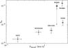 |
Fig. 8 Inner water abundance vs. the absolute value of the infall or expansion velocity as derived from our model (see Table 8). The filled square symbol is for W3IRS5 from Chavarría et al. (2010), and the arrow shows the abundance for W3IRS5 from van der Tak et al. (2006). |
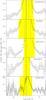 |
Fig. 9 Line ratio of the CH3OH 51,5−40,4A+−A+ over the p-H2O 202−111 transition, both rebinned to 0.5 kms-1. The VLSR is shown with a dashed line. The range of velocities where the high optical depth of the water is assumed to affect the derived ratio is shown in yellow. |
Another explanation of the low inner abundance might be that photodissociation through protostellar UV photons is more efficient than expected and thus not completely outrun by the O→H2O conversion. In the presence of strong UV radiation fields like the internal extreme UV radiation from the surface of a massive star (e.g., 3 × 1038 erg s-1, Benz et al. 2013), water vapor is photodissociated. The physical known characteristics of our sources (see Table 1) do not indicate any difference in terms of FUV internal field among our sample, but we can imagine that for some reasons (e.g., self-shielding due to the thickness of the inner region), water photodissociation is more efficient in IRAS 16272 than in W43-MM1, for instance. Observing good FUV irradiation tracers such as OH+ or CH+, or the product of the water photodissociation, that is, OH, might help to constrain this scenario.
7.2. Methanol and the formation route of water at higher velocities
Of the various species detected in our spectra (see Tables B.1−B.5), the methanol lines are important indicators of the physical conditions in the protostellar envelope because they are so numerous. The observed line ratio of CH3OH over water as a function of the velocity in the line wings is able to differentiate between two potential formation routes of H2O, gas-phase synthesis versus a sputtered origin in the outflow (Suutarinen et al. 2014). van Kempen et al. (2014) have shown that in intermediate-mass protostars organic molecules (e.g., the pure grain mantle product CH3OH) most likely originate from sputtering of ices through outflow shocks and cannot form through gas-phase synthesis, as opposed to H2O. In contrast to the water lines, most of the CH3OH lines detected in our sample do not exhibit a broad component, but rather a medium velocity component. Hence, comparison of water and CH3OH velocity components (e.g., see Fig. B.4) shows that methanol does not trace exactly the same gas as the broad water component, or that the abundance ratio is much lower in the shocks. Of the detected methanol lines with a good S/N, we compared the CH3OH lines, whose upper energy level is similar (Eu ≤ 105 K, 51,5−40,4A+−A+, 63,4−52,3A+−A+, 63,3−52,4A−−A−, and 81,7−70,7E) to the p-H2O 202−111 line. All transitions were assumed to fill the beam. Following van Kempen et al. (2014), we did not consider a range of velocities around the line center, where the significant optical depth in the water lines increases the line ratio much more than physical processes would. As explained in Sect. 5.4, considering the high critical densities of water transitions, we assumed effectively thin emission away from this central line region (according to Suutarinen et al. 2014, the effect of water opacity on the ratio is still weak).
Figure 9 shows the ratio for the CH3OH 51,5−40,4A+−A+ over the p-H2O 202−111 transitions. Except for IRAS 05358, where the methanol line shows no wing, the ratio clearly drops as a function of velocity in both wings (although fewer channels in the red wing are unaffected by the optical depth), suggesting a dominant gas-phase synthesis of H2O from shocked material because methanol is produced on grain surfaces. Line ratios of other CH3OH lines over the same H2O line (or p-H2O 211−202) show the same behavior. We therfore conclude that high-velocity water must be formed in the gas-phase from shocked material, meaning that it is not created solely through grain mantle evaporation.
7.3. Star formation processes and evolution
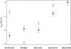 |
Fig. 10 Infall velocity vs. evolutionary sequence. Red triangles and filled blue squares represent H2O and CS (see Appendix D) velocities. |
Observed fluxes and luminosities for all lines and sources.
Turbulence, infall, and outflow are important ingredients of the star formation process. We confirm here that the observed molecular emission in massive protostellar objects is dominated by supersonic turbulent velocities (see Fig. 7) at all radii. Hence regions of massive-star formation are highly turbulent. This supersonic turbulence agrees with the turbulent core model of McKee & Tan (2003), but is also consistent with the competitive accretion scenario in which local velocity dispersions are small, but line-of-sight velocities can be significantly higher as a result of the fragmentation of the cloud (Bonnell & Bate 2006). Moreover, our results indicate that the turbulent motions tend to increase with radius, consistent again with all models (see Bonnell & Bate 2006; McKee & Tan 2003). Nevertheless, rotation and non-spherical density structure cannot be excluded as possible explanations (see Herpin et al. 2012), and accurate estimates of the turbulence also require careful subtraction of cold foreground clouds in some cases (Jacq et al., in prep.).
Assuming isotropic radiation, we estimate the lower limit to the total HIFI water luminosity by adding all individual observed luminosities to be 16.8, 33.1, 23.9, and 14.4 L⊙ in our sources (evolutionary order) based on the integrated fluxes of components in emission in observed lines (Table 9). This confirms the low contribution of water cooling to the total far-IR gas cooling compared to the cooling from other species (Karska et al. 2014). The true water emission from the inner part may be much higher, but the cool envelope absorbs much of the emission. Based on the modeling, we moreover estimate the total water mass in the envelope (see Table 8) to roughly 8−9 × 10⁻⁴M⊙ for NGC 6334I(N) and DR21(OH), and 10-4M⊙ for the two other objects. The fraction of the water mass to the envelope mass differs by more than an order of magnitude from source to source (0.6 × 10⁻⁷ to 16.3 × 10⁻⁷). The proportion of the mass in the inner part is only 3.6% for NGC 6334I(N) and 11.8% for DR21(OH), but increases to 26.7% and 43.8% for the more evolved objects IRAS 05358 and IRAS 16272.
If the whole envelope mass (see Table 1) were collapsing, infall velocities from 2.1 kms-1 for IRAS 05358 to up to 9.7 kms-1 for NGC 6334I(N) would be expected assuming free-fall accretion. This is higher by up to a factor of 10 than what we estimate here (we even detect no infall in IRAS 05358, consistent with HCO+ observations of Klaassen et al. 2012). The free-fall accretion rate (monolithic collapse, Shu 1977) is 6.3 × 10⁻⁶M⊙/yr for sound speed of 0.3 kms-1 (a few 10-5M⊙/yr for temperatures above 100 K), which is several orders of magnitude lower than what we derived from our observations (see Table 8). We note that the CS infall velocity provides another estimate of the mass accretion rate (see Table D.1 in Appendix D), approximately 50% lower than the values inferred from the water lines. Models of star formation based on gravoturbulent fragmentation (Schmeja & Klessen 2004) predict mass accretion rates of 3.4 × 10⁻⁵M⊙/yr (same sound speed of gas), but varying with time, while this rate is constant in the standard theory of isolated star formation from Shu (1977). Of course, these accretion rates from our calculations assume spherical accretion and one central object, which might not be true. Nevertheless, these rates are similar to those derived from the turbulent core model for massive molecular cloud cores dominated by supersonic turbulence (a few 10-5−10-4M⊙/yr, McKee & Tan 2003) and from the competitive accretion model that can produce accretion rates from 10-9 to 10-4M⊙/yr (depending on the gas density and initial stellar and fragment mass). Models of gravitational collapse of massive magnetized molecular cloud cores (e.g., Banerjee & Pudritz 2007) generate massive star formation through high accretion rates (that can exceed 10-3M⊙/yr) and disk-driven outflows.
Considering a typical mass of 20 M⊙ within a radius of 100 R⋆, we estimate the corresponding accretion luminosity of a protostar from Hosokawa et al. (2010) using 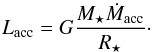 (2)The derived luminosities (see Table 8), compared to the observed total luminosity (stellar+accretion, Table 1), seem unrealistically high for W43-MM1 and NGC 6334I(N), but we stress that the scales of infall probed by water and the accretion onto the protostars are probably quite different: we here probe infall in the envelope and not accretion onto the protostar. However, using the lower values derived from CS observations, the accretion luminosities are compatible with the observed total luminosity, therefore we suggest that water may not be a good accretion tracer. Moreover, the derived accretion rate, although uncertain, is high enough for W43-MM1 and NGC 6334I(N) to overcome the radiation pressure that is due to the stellar luminosity (see Table 9). This is possibly true for DR21(OH) as well, but not for IRAS 16272 (no accretion is detected in IRAS 05358). Nevertheless, the simple comparison of radiation pressure and mass accretion rate in the simple one-dimensional collapse model view is considered as insufficient to explain the observations (Peters et al. 2010).
Beyond the classical monolithic collapse and competitive accretion model, Peters et al. (2010) proposed the collapse of a rotating massive cloud core involving a process called fragmentation-induced starvation to reproduce the strong clumping and filamentary structures observed in collapsing cores. According to this model, the accretion decreases with time (between 10-3 and 10-5M⊙/yr), consistent with results from Peters et al. (2010). But considering the evolutionary sequence described in Sect. 3, the accretion rates derived for our sample (Table 8) do not show any trend.
Because of the different level of fragmentation or substructure in our source sample, comparing estimates of the mass accretion rates along the evolutionary sequence of this sample is uncertain. Nevertheless, the infall velocity derived from H2O (except for NGC 6334IN) and CS observations tends to decrease with the evolutionary stage of the massive object (Fig. 10).
8. Conclusions
We have presented Herschel-HIFI observations of 14 far-IR water lines (HO, HO, HO) toward four mid-IR quiet massive protostellar objects, assumed to be at the beginning of the high-mass star formation process, and ordered them in terms of an evolutionary sequence based on their SED. We studied the envelope kinematics (outflow, infall, turbulent velocity) from the different components identified in the line profiles of our source sample and derived the water abundances using the RATRAN radiative transfer code. In addition, our analysis was supplemented in terms of “evolution” and water formation by the serendipitous detection of several other molecular lines, especially CS and methanol.
The water lines have broad, medium, and narrow velocity components, while no envelope component was found in W43-MM1 by Herpin et al. (2012). The more evolved sources, IRAS 05358 and IRAS 16272, exhibit fewer and weaker rare isotopolog lines and appear to be less rich chemically, as indicated by the number of serendipitous species detected in these observations. We confirm that regions of massive star formation are highly turbulent and that turbulence tends to increase in the envelope with the distance to the star, as seen in W43-MM1 by Herpin et al. (2012). This trend is consistent with the supersonic turbulent core model, which leads to high-mass star formation in the presence of a disk, although these constraints are also consistent with competitive accretion.
The whole set of lines allowed us to constrain the outer water abundance by modeling to the typical value of a few 10-8 , while we infer 1.7 × 10⁻⁶−1.4 × 10⁻⁴ for the inner abundance, which is lower (except for W43-MM1) than expected from ice evaporation. Possible explanations might be that (i) photodissociation of water from the UV internal photons of the massive protostar is more efficient than expected, or that (ii) our simple spherical envelope model underestimates the inner water abundance. Moreover, we showed that the higher the infall or expansion velocity in the protostellar envelope, the higher the inner abundance. This fact, in addition to the observed lower infall velocity along the source evolutionary sequence, suggests that younger sources with higher infall or expansion velocities may generate shocks that will sputter water from the ice mantles of dust grains in the inner region. At high velocities, water must be formed in the gas phase from shocked material, or in other words, it is not created solely through grain mantle evaporation.
Acknowledgments
This program was made possible thanks to the HIFI guaranteed time. HIFI has been designed and built by a consortium of institutes and university departments from across Europe, Canada and the United States under the leadership of SRON Netherlands Institute for Space Research, Groningen, The Netherlands and with major contributions from Germany, France and the US. Consortium members are: Canada: CSA, U.Waterloo; France: CESR, LAB, LERMA, IRAM; Germany: KOSMA, MPIfR, MPS; Ireland, NUI Maynooth; Italy: ASI, IFSI-INAF, Osservatorio Astrofisico di Arcetri- INAF; Netherlands: SRON, TUD; Poland: CAMK, CBK; Spain: Observatorio Astronomico Nacional (IGN), Centro de Astrobiologi (CSIC-INTA). Sweden: Chalmers University of Technology − MC2, RSS & GARD; Onsala Space Observatory; Swedish National Space Board, Stockholm University − Stockholm Observatory; Switzerland: ETH Zurich, FHNW; USA: Caltech, JPL, NHSC. HIPE is a joint development by the Herschel Science Ground Segment Consortium, consisting of ESA, the NASA Herschel Science Center, and the HIFI, PACS and SPIRE consortia. Astrochemistry in Leiden is supported by the Netherlands Research School for Astronomy (NOVA), by a Spinoza grant and grant 614.001.008 from the Netherlands Organisation for Scientific Research (NWO), and by the European Community’s Seventh Framework Program FP7/2007-2013 under grant agreement 238258 (LASSIE). We also thank the French Space Agency CNES for financial support. We thank J. Mottram for useful comments and discussions.
References
- Aikawa, Y., Wakelam, V., Garrod, R. T., & Herbst, E. 2008, ApJ, 674, 984 [NASA ADS] [CrossRef] [Google Scholar]
- Araya, E. D., Kurtz, S., Hofner, P., & Linz, H. 2009, ApJ, 698, 1321 [NASA ADS] [CrossRef] [Google Scholar]
- Banerjee, R., & Pudritz, R. E. 2007, ApJ, 660, 479 [NASA ADS] [CrossRef] [Google Scholar]
- Benz, A. O., Bruderer, S., van Dishoeck, E. F., et al. 2010, A&A, 521, L35 [NASA ADS] [CrossRef] [EDP Sciences] [Google Scholar]
- Benz, A. O., Bruderer, S., van Dishoeck, E. F., Stäuber, P., & Wampfler, S. F. 2013, J. Phys. Chem. A, 117, 9840 [CrossRef] [Google Scholar]
- Beuther, H., Schilke, P., Gueth, F., et al. 2002a, A&A, 387, 931 [NASA ADS] [CrossRef] [EDP Sciences] [Google Scholar]
- Beuther, H., Schilke, P., Menten, K. M., et al. 2002b, ApJ, 566, 945 [NASA ADS] [CrossRef] [Google Scholar]
- Beuther, H., Leurini, S., Schilke, P., et al. 2007, A&A, 466, 1065 [NASA ADS] [CrossRef] [EDP Sciences] [Google Scholar]
- Beuther, H., Walsh, A. J., Thorwirth, S., et al. 2008, A&A, 481, 169 [NASA ADS] [CrossRef] [EDP Sciences] [Google Scholar]
- Bonnell, I. A., & Bate, M. R. 2006, MNRAS, 370, 488 [NASA ADS] [CrossRef] [Google Scholar]
- Bontemps, S., Andre, P., Terebey, S., & Cabrit, S. 1996, A&A, 311, 858 [NASA ADS] [Google Scholar]
- Boonman, A. M. S., Doty, S. D., van Dishoeck, E. F., et al. 2003, A&A, 406, 937 [NASA ADS] [CrossRef] [EDP Sciences] [Google Scholar]
- Brogan, C. L., Hunter, T. R., Cyganowski, C. J., et al. 2009, ApJ, 707, 1 [NASA ADS] [CrossRef] [Google Scholar]
- Bruderer, S., Benz, A. O., van Dishoeck, E. F., et al. 2010, A&A, 521, L44 [NASA ADS] [CrossRef] [EDP Sciences] [Google Scholar]
- Ceccarelli, C., Bacmann, A., Boogert, A., et al. 2010, A&A, 521, L22 [NASA ADS] [CrossRef] [EDP Sciences] [Google Scholar]
- Chandler, C. J., Moore, T. J. T., Mountain, C. M., & Yamashita, T. 1993, MNRAS, 261, 694 [NASA ADS] [Google Scholar]
- Charnley, S. B. 1997, ApJ, 481, 396 [NASA ADS] [CrossRef] [Google Scholar]
- Chavarría, L., Herpin, F., Jacq, T., et al. 2010, A&A, 521, L37 [NASA ADS] [CrossRef] [EDP Sciences] [Google Scholar]
- Cortes, P. C. 2011, ApJ, 743, 194 [NASA ADS] [CrossRef] [Google Scholar]
- Csengeri, T., Bontemps, S., Schneider, N., et al. 2011, ApJ, 740, L5 [NASA ADS] [CrossRef] [Google Scholar]
- Daniel, F., Dubernet, M.-L., & Grosjean, A. 2011, A&A, 536, A76 [NASA ADS] [CrossRef] [EDP Sciences] [Google Scholar]
- de Graauw, T., Helmich, F. P., Phillips, T. G., et al. 2010, A&A, 518, L6 [NASA ADS] [CrossRef] [EDP Sciences] [Google Scholar]
- Emprechtinger, M., Lis, D. C., Rolffs, R., et al. 2013, ApJ, 765, 61 [NASA ADS] [CrossRef] [Google Scholar]
- Faúndez, S., Bronfman, L., Garay, G., et al. 2004, A&A, 426, 97 [NASA ADS] [CrossRef] [EDP Sciences] [Google Scholar]
- Fraser, H. J., Collings, M. P., McCoustra, M. R. S., & Williams, D. A. 2001, MNRAS, 327, 1165 [NASA ADS] [CrossRef] [Google Scholar]
- Fuller, G. A., Williams, S. J., & Sridharan, T. K. 2005, A&A, 442, 949 [NASA ADS] [CrossRef] [EDP Sciences] [Google Scholar]
- Garay, G., Mardones, D., Brooks, K. J., Videla, L., & Contreras, Y. 2007, ApJ, 666, 309 [NASA ADS] [CrossRef] [Google Scholar]
- Gerner, T., Beuther, H., Semenov, D., et al. 2014, A&A, 563, A97 [NASA ADS] [CrossRef] [EDP Sciences] [Google Scholar]
- Girart, J. M., Frau, P., Zhang, Q., et al. 2013, ApJ, 772, 69 [NASA ADS] [CrossRef] [Google Scholar]
- Goldsmith, P. F., & Langer, W. D. 1999, ApJ, 517, 209 [NASA ADS] [CrossRef] [Google Scholar]
- Harvey, P. M., Joy, M., Lester, D. F., & Wilking, B. A. 1986, ApJ, 300, 737 [NASA ADS] [CrossRef] [Google Scholar]
- Heitsch, F., Hartmann, L. W., Slyz, A. D., Devriendt, J. E. G., & Burkert, A. 2008, ApJ, 674, 316 [NASA ADS] [CrossRef] [Google Scholar]
- Helmich, F. P., van Dishoeck, E. F., Black, J. H., et al. 1996, A&A, 315, L173 [NASA ADS] [Google Scholar]
- Hennemann, M., Motte, F., Schneider, N., et al. 2012, A&A, 543, L3 [NASA ADS] [CrossRef] [EDP Sciences] [Google Scholar]
- Herpin, F., Marseille, M., Wakelam, V., Bontemps, S., & Lis, D. C. 2009, A&A, 504, 853 [NASA ADS] [CrossRef] [EDP Sciences] [Google Scholar]
- Herpin, F., Chavarría, L., van der Tak, F., et al. 2012, A&A, 542, A76 [NASA ADS] [CrossRef] [EDP Sciences] [Google Scholar]
- Hogerheijde, M. R., & van der Tak, F. F. S. 2000, A&A, 362, 697 [NASA ADS] [Google Scholar]
- Hosokawa, T., Yorke, H. W., & Omukai, K. 2010, ApJ, 721, 478 [NASA ADS] [CrossRef] [Google Scholar]
- Hunter, T. R., Brogan, C. L., Megeath, S. T., et al. 2006, ApJ, 649, 888 [NASA ADS] [CrossRef] [Google Scholar]
- Hunter, T. R., Brogan, C. L., Cyganowski, C. J., & Young, K. H. 2014, ApJ, 788, 187 [NASA ADS] [CrossRef] [Google Scholar]
- Jacq, T., Walmsley, C. M., Henkel, C., et al. 1990, A&A, 228, 447 [NASA ADS] [Google Scholar]
- Johnstone, D., Fich, M., McCoey, C., et al. 2010, A&A, 521, L41 [NASA ADS] [CrossRef] [EDP Sciences] [Google Scholar]
- Karska, A., Herpin, F., Bruderer, S., et al. 2014, A&A, 562, A45 [NASA ADS] [CrossRef] [EDP Sciences] [Google Scholar]
- Kaźmierczak-Barthel, M., Semenov, D. A., van der Tak, F. F. S., Chavarría, L., & van der Wiel, M. H. D. 2015, A&A, 574, A71 [NASA ADS] [CrossRef] [EDP Sciences] [Google Scholar]
- Klaassen, P. D., Testi, L., & Beuther, H. 2012, A&A, 538, A140 [NASA ADS] [CrossRef] [EDP Sciences] [Google Scholar]
- Kristensen, L. E., Visser, R., van Dishoeck, E. F., et al. 2010, A&A, 521, L30 [NASA ADS] [CrossRef] [EDP Sciences] [Google Scholar]
- Krumholz, M. R., McKee, C. F., & Klein, R. I. 2005, ApJ, 618, L33 [NASA ADS] [CrossRef] [Google Scholar]
- Krumholz, M. R., & Bonnell, I. A. 2009, Models for the formation of massive stars, ed. G. Chabrier (Cambridge University Press), 288 [Google Scholar]
- Kuiper, R., Klahr, H., Beuther, H., & Henning, T. 2010, ApJ, 722, 1556 [CrossRef] [Google Scholar]
- Kuiper, R., Yorke, H. W., & Turner, N. J. 2015, ApJ, 800, 86 [NASA ADS] [CrossRef] [Google Scholar]
- Lester, D. F., Dinerstein, H. L., Werner, M. W., et al. 1985, ApJ, 296, 565 [NASA ADS] [CrossRef] [Google Scholar]
- Leurini, S., Beuther, H., Schilke, P., et al. 2007, A&A, 475, 925 [NASA ADS] [CrossRef] [EDP Sciences] [Google Scholar]
- Marseille, M. G., van der Tak, F. F. S., Herpin, F., & Jacq, T. 2010a, A&A, 522, A40 [NASA ADS] [CrossRef] [EDP Sciences] [Google Scholar]
- Marseille, M. G., van der Tak, F. F. S., Herpin, F., et al. 2010b, A&A, 521, L32 [Google Scholar]
- McCutcheon, W. H., Sandell, G., Matthews, H. E., et al. 2000, MNRAS, 316, 152 [NASA ADS] [CrossRef] [Google Scholar]
- McKee, C. F., & Tan, J. C. 2003, ApJ, 585, 850 [NASA ADS] [CrossRef] [MathSciNet] [Google Scholar]
- Motte, F., Schilke, P., & Lis, D. C. 2003, ApJ, 582, 277 [NASA ADS] [CrossRef] [Google Scholar]
- Motte, F., Bontemps, S., Schilke, P., et al. 2007, A&A, 476, 1243 [NASA ADS] [CrossRef] [EDP Sciences] [Google Scholar]
- Mottram, J. C., Hoare, M. G., Davies, B., et al. 2011, ApJ, 730, L33 [NASA ADS] [CrossRef] [Google Scholar]
- Mottram, J. C., Kristensen, L. E., van Dishoeck, E. F., et al. 2014, A&A, 572, A21 [NASA ADS] [CrossRef] [EDP Sciences] [Google Scholar]
- Muñoz, D. J., Mardones, D., Garay, G., et al. 2007, ApJ, 668, 906 [NASA ADS] [CrossRef] [Google Scholar]
- Neufeld, D. A., Gusdorf, A., Güsten, R., et al. 2014, ApJ, 781, 102 [NASA ADS] [CrossRef] [Google Scholar]
- Ott, S. 2010, in Astronomical Data Analysis Software and Systems XIX, eds. Y. Mizumoto, K.-I. Morita, & M. Ohishi, ASP Conf. Ser., 434, 139 [Google Scholar]
- Palau, A., Estalella, R., Girart, J. M., et al. 2014, ApJ, 785, 42 [NASA ADS] [CrossRef] [Google Scholar]
- Pearson, J. C., De Lucia, F. C., Anderson, T., Herbst, E., & Helminger, P. 1991, ApJ, 379, L41 [NASA ADS] [CrossRef] [Google Scholar]
- Peters, T., Klessen, R. S., Mac Low, M.-M., & Banerjee, R. 2010, ApJ, 725, 134 [NASA ADS] [CrossRef] [Google Scholar]
- Pilbratt, G. L., Riedinger, J. R., Passvogel, T., et al. 2010, A&A, 518, L1 [CrossRef] [EDP Sciences] [Google Scholar]
- Ragan, S., Henning, T., Krause, O., et al. 2012, A&A, 547, A49 [NASA ADS] [CrossRef] [EDP Sciences] [Google Scholar]
- Richardson, K. J., Sandell, G., Cunningham, C. T., & Davies, S. R. 1994, A&A, 286, 555 [NASA ADS] [Google Scholar]
- Roberts, J. F., Rawlings, J. M. C., & Stace, H. A. 2010, MNRAS, 408, 2426 [NASA ADS] [CrossRef] [Google Scholar]
- Rodríguez, L. F., Zapata, L. A., & Ho, P. T. P. 2007, ApJ, 654, L143 [NASA ADS] [CrossRef] [Google Scholar]
- Roelfsema, P. R., Helmich, F. P., Teyssier, D., et al. 2012, A&A, 537, A17 [NASA ADS] [CrossRef] [EDP Sciences] [Google Scholar]
- San José-García, I., Mottram, J. C., Kristensen, L. E., et al. 2013, A&A, 553, A125 [NASA ADS] [CrossRef] [EDP Sciences] [Google Scholar]
- San Jose-Garcia, I., Mottram, J. C., van Dishoeck, E. F., et al. 2016, A&A, 585, A103 [NASA ADS] [CrossRef] [EDP Sciences] [Google Scholar]
- Sandell, G. 2000, A&A, 358, 242 [NASA ADS] [Google Scholar]
- Schlingman, W. M., Shirley, Y. L., Schenk, D. E., et al. 2011, ApJS, 195, 14 [NASA ADS] [CrossRef] [Google Scholar]
- Schmalzl, M., Visser, R., Walsh, C., et al. 2014, A&A, 572, A81 [NASA ADS] [CrossRef] [EDP Sciences] [Google Scholar]
- Schmeja, S., & Klessen, R. S. 2004, A&A, 419, 405 [NASA ADS] [CrossRef] [EDP Sciences] [Google Scholar]
- Shipman, R. F., van der Tak, F. F. S., Wyrowski, F., Herpin, F., & Frieswijk, W. 2014, A&A, 570, A51 [Google Scholar]
- Shirley, Y. L., Evans, II, N. J., Young, K. E., Knez, C., & Jaffe, D. T. 2003, ApJS, 149, 375 [NASA ADS] [CrossRef] [Google Scholar]
- Shu, F. H. 1977, ApJ, 214, 488 [NASA ADS] [CrossRef] [Google Scholar]
- Snell, R. L., Howe, J. E., Ashby, M. L. N., et al. 2000, ApJ, 539, L101 [NASA ADS] [CrossRef] [Google Scholar]
- Suutarinen, A. N., Kristensen, L. E., Mottram, J. C., Fraser, H. J., & van Dishoeck, E. F. 2014, MNRAS, 440, 1844 [NASA ADS] [CrossRef] [Google Scholar]
- Tan, J. C., Beltrán, M. T., Caselli, P., et al. 2014, Protostars and Planets VI, 149 [Google Scholar]
- Tan, J. C., & McKee, C. F. 2002, in Hot Star Workshop III: The Earliest Phases of Massive Star Birth, ed. P. Crowther, ASP Conf. Ser., 267, 267 [Google Scholar]
- Thomas, H. S., & Fuller, G. A. 2008, A&A, 479, 751 [NASA ADS] [CrossRef] [EDP Sciences] [Google Scholar]
- Vallée, J. P., & Fiege, J. D. 2006, ApJ, 636, 332 [NASA ADS] [CrossRef] [Google Scholar]
- van der Tak, F. F. S., van Dishoeck, E. F., Evans, II, N. J., & Blake, G. A. 2000, ApJ, 537, 283 [NASA ADS] [CrossRef] [Google Scholar]
- van der Tak, F. F. S., Walmsley, C. M., Herpin, F., & Ceccarelli, C. 2006, A&A, 447, 1011 [NASA ADS] [CrossRef] [EDP Sciences] [Google Scholar]
- van der Tak, F. F. S., Black, J. H., Schöier, F. L., Jansen, D. J., & van Dishoeck, E. F. 2007, A&A, 468, 627 [NASA ADS] [CrossRef] [EDP Sciences] [Google Scholar]
- van der Tak, F. F. S., Marseille, M. G., Herpin, F., et al. 2010, A&A, 518, L107 [Google Scholar]
- van der Tak, F. F. S., Chavarría, L., Herpin, F., et al. 2013, A&A, 554, A83 [NASA ADS] [CrossRef] [EDP Sciences] [Google Scholar]
- van der Wiel, M. H. D., Pagani, L., van der Tak, F. F. S., Kaźmierczak, M., & Ceccarelli, C. 2013, A&A, 553, A11 [NASA ADS] [CrossRef] [EDP Sciences] [Google Scholar]
- van Dishoeck, E. F., & Helmich, F. P. 1996, A&A, 315, L177 [NASA ADS] [Google Scholar]
- van Dishoeck, E. F., Kristensen, L. E., Benz, A. O., et al. 2011, PASP, 123, 138 [NASA ADS] [CrossRef] [Google Scholar]
- van Dishoeck, E. F., Herbst, E., & Neufeld, D. A. 2013, Chem. Rev., 113, 9043 [NASA ADS] [CrossRef] [PubMed] [Google Scholar]
- van Kempen, T. A., McCoey, C., Tisi, S., Johnstone, D., & Fich, M. 2014, A&A, 569, A53 [Google Scholar]
- Vázquez-Semadeni, E., Gómez, G. C., Jappsen, A. K., et al. 2007, ApJ, 657, 870 [NASA ADS] [CrossRef] [Google Scholar]
- Villanueva, G. L., DiSanti, M. A., Mumma, M. J., & Xu, L.-H. 2012, ApJ, 747, 37 [NASA ADS] [CrossRef] [Google Scholar]
- Visser, R., Jørgensen, J. K., Kristensen, L. E., van Dishoeck, E. F., & Bergin, E. A. 2013, ApJ, 769, 19 [NASA ADS] [CrossRef] [Google Scholar]
- Walsh, A. J., Burton, M. G., Hyland, A. R., & Robinson, G. 1998, MNRAS, 301, 640 [NASA ADS] [CrossRef] [Google Scholar]
- Wilson, T. L., & Rood, R. 1994, ARA&A, 32, 191 [NASA ADS] [CrossRef] [Google Scholar]
- Woody, D. P., Scott, S. L., Scoville, N. Z., et al. 1989, ApJ, 337, L41 [NASA ADS] [CrossRef] [Google Scholar]
- Wu, J., Evans, II, N. J., Shirley, Y. L., & Knez, C. 2010, ApJS, 188, 313 [NASA ADS] [CrossRef] [Google Scholar]
- Wyrowski, F., van der Tak, F., Herpin, F., et al. 2010, A&A, 521, L34 [NASA ADS] [CrossRef] [EDP Sciences] [Google Scholar]
- Yorke, H. W., & Sonnhalter, C. 2002, ApJ, 569, 846 [NASA ADS] [CrossRef] [Google Scholar]
- Zapata, L. A., Loinard, L., Su, Y.-N., et al. 2012, ApJ, 744, 86 [NASA ADS] [CrossRef] [Google Scholar]
- Zinnecker, H., & Yorke, H. W. 2007, ARA&A, 45, 481 [NASA ADS] [CrossRef] [Google Scholar]
Appendix A: AOR list
AORs list of Herschel observations for each source.
Appendix B: By-product lines
Observed line emission parameters for the serendipitously detected lines toward IRAS 05358.
Observed line emission parameters for the serendipitously detected lines toward IRAS 16272.
Observed line emission parameters for the serendipitously detected lines toward NGC 6334I(N).
Observed line emission parameters for the serendipitously detected lines toward W43-MM1.
Observed line emission parameters for the serendipitously detected lines toward DR21(OH).
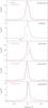 |
Fig. B.1 HIFI spectra of 13CO J = 5−4 (black) and 10−9 lines (red). The spectra have been smoothed to 0.2 kms-1. Vertical dotted lines indicate the VLSR. |
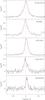 |
Fig. B.2 HIFI spectra of the CS J = 11−10 line. The best-fit model is shown in red overlaid on the spectra. Vertical dotted lines indicate the VLSR. The spectra have been smoothed to 0.2 kms-1. |
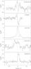 |
Fig. B.3 HIFI spectra of H2S 30,3−21,2 line (blended with the H2S 30,3−21,2 line at 993.09701 GHz). The spectra have been smoothed to 0.2 kms-1. Vertical dotted lines indicate the VLSR. |
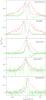 |
Fig. B.4 HIFI nomalized spectra of CH3OH 51,5−40,4A+−A+ line (in black) overplotted on the p-H2O 202−111 (red) and p-H |
Appendix C: Gaussian fit components for IRAS 05358
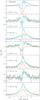 |
Fig. C.1 Gaussian fit components (red, blue, and green) for H |
Appendix D: CS distribution
We also applied the model to the CS 11−10 line. In addition, we tried to reproduce other CS lines observed by other authors: J = 7−6 for W43-MM1 (Herpin et al. 2009) and NGC 6334I(N) (McCutcheon et al. 2000), J = 5−4 for IRAS 05358 and W43-MM1 (Herpin et al. 2009), DR21(OH) (Richardson et al. 1994), J = 3−2 for IRAS 05358 (Herpin et al. 2009), and J = 2−1 for IRAS 16272 (Mopra observation, Herpin et al., priv. comm.). This showed that the sources IRAS 05358 and W43-MM1 are best constrained because they have the most available CS lines. Results for CS 11−10 line are shown in Fig. B.2. For all sources but DR21(OH), a jump in abundance is necessary to reproduce the lower-J CS lines (7−6, 5−4, 3−2, and 2−1). The CS inner abundance is 4 × 10⁻⁸ for IRAS 05358, IRAS 16272, and DR21(OH), while the abundance is lower for NGC 6334I(N) (an order of magnitude: 4 × 10⁻⁹) and W43-MM1 (9 × 10⁻⁹). All parameters are given in Table D.1. We first modeled the CS 11−10 line solely with constant turbulent and infall velocities, but, as for water, adopting a turbulence increasing with radius (but constant infall) improves the line fitting, especially when including the other CS lines. The resulting Vturb profiles are overplotted in Fig. 7 with turbulence inferred from water lines, but they need to be considered with caution as the CS model is less well constrained than that of water because significantly fewer lines are involved in the process. The variation of these two turbulent velocities is not strictly identical, the obvious difference being a lower turbulence for CS lines. This might be consistent with CS not tracing exactly the same gas as water lines because it is located more in the inner part of the envelope where the turbulence is weaker: as proposed in Sect. 7.2, water is produced by gas-phase synthesis of H2O from shocked material in the outflow cavity, which is probably not true for CS.
Compared to previous publications, our CS abundances are larger by almost two orders of magnitude for IRAS 05358 (Herpin et al. 2009) and DR21(OH) (Richardson et al. 1994), but they are consistent with those reported by Cortes (2011) for W43-MM1. These CS abundances agree with predictions from chemical models (Roberts et al. 2010): the lower CS abundance in the less evolved mid-IR quiet sources, NGC 6334I(N) and W43-MM1, might indicate than CS is depleted on the grain mantles in these younger objects. The abundance of CS is dependent on the evaporation of sulfur from the ice mantles by radiation from the central star.
CS parameters derived from the model.
Appendix E: Methanol lines
Based on the CH3OH (vt = 0) integrated lines fluxes that were corrected for the beam dilution (reference beam is 21.1″) and assuming LTE, we made rotational diagrams for all sources (see Fig. E.1) up to Eup/kB = 440 K for DR21(OH) and W43-MM1, and up to Eup/kB = 200 K for IRAS 16272 and IRAS 05358. We estimated the rotational temperature and the total methanol column density using the partition function from Villanueva et al. (2012). All rotational diagrams can be described by a single temperature, but ln(Nup/gup) values are scattered for W43-MM1 and IRAS 16272 either because of opacity effects or non-LTE conditions. Even for our very limited sample of methanol transitions, we attempted to iteratively correct individual Nup/gup values by muliplying by the optical depth correction factor after the method of Goldsmith & Langer (1999). We find that the corrected optical depth is always ≪1, and the correction factors are lower than 1%. Taking into account the uncertainties, we note that the rotational temperature possibly increases with the evolutionary sequence assumed in this paper, which would underline the increasing temperature in the protostellar envelope. Beam-averaged methanol column densities are a few 1015 cm-2 for all sources, except for DR21(OH), where the column density is one order of magnitude higher. The fact that we detect torsionally excited methanol lines (v = 1) in DR21(OH) and W43-MM1 and that the number of detected CH3OH lines increases with the source luminosity reveals the role of the IR pumping for the methanol emission (Leurini et al. 2007).
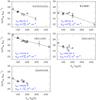 |
Fig. E.1 Rotational diagrams for methanol lines (vt = 0). Sources are ordered following the evolutionary sequence. |
All Tables
Observed line emission parameters for the detected water lines toward IRAS 05358.
HO integrated line intensity ratios (not corrected for different beam sizes) for all sources for the broad velocity component.
Observed line emission parameters for the serendipitously detected lines toward IRAS 05358.
Observed line emission parameters for the serendipitously detected lines toward IRAS 16272.
Observed line emission parameters for the serendipitously detected lines toward NGC 6334I(N).
Observed line emission parameters for the serendipitously detected lines toward W43-MM1.
Observed line emission parameters for the serendipitously detected lines toward DR21(OH).
All Figures
|
Fig. 1 Spectral energy distributions obtained from the 1D model overlaid on observed flux densities of each source. Peak flux densities in the millimeter range have been adjusted to fit the radial extent of the model. Each caption gives the temperatures of the black body components (top right), the maximum flux Fmax, and the corresponding wavelength of the SED, the flux F12 at 12 μm, and the contribution of the hot part (F35, integrated flux for λ< 35 μm) to the total integrated flux Ftotal (top left). |
| In the text | |
|
Fig. 2 HIFI spectra of H |
| In the text | |
|
Fig. 3 As in Fig. 2, but for DR21(OH) (Vinf = −1.5 and Vturb = 2.5 kms-1 for the constant model). The p-H2O 524−431 line is blended with the CH3OH line at 957.995737 GHz from the LSB. |
| In the text | |
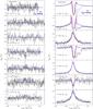 |
Fig. 4 As in Fig. 2, but for IRAS 16272 (Vinf = −0.2 and Vturb = 2.2 kms-1 for the constant model). |
| In the text | |
|
Fig. 5 As in Fig. 2, but for IRAS 05358 (Vinf = + 3.0 and Vturb = 2.0 kms-1 for the constant model), more (in green) a varying outer abundance model (see Sect. 6.3) |
| In the text | |
|
Fig. 6 FWHM versus offset of the peak from the source velocity for the Gaussian velocity components found in the water (H |
| In the text | |
|
Fig. 7 Variation of the turbulent velocity Vturb with the distance R (AU) to the central object as derived from the model for water (in black) and CS (in red, see Appendix D). Error bars illustrate the range of values that has no impact on the model. |
| In the text | |
|
Fig. 8 Inner water abundance vs. the absolute value of the infall or expansion velocity as derived from our model (see Table 8). The filled square symbol is for W3IRS5 from Chavarría et al. (2010), and the arrow shows the abundance for W3IRS5 from van der Tak et al. (2006). |
| In the text | |
|
Fig. 9 Line ratio of the CH3OH 51,5−40,4A+−A+ over the p-H2O 202−111 transition, both rebinned to 0.5 kms-1. The VLSR is shown with a dashed line. The range of velocities where the high optical depth of the water is assumed to affect the derived ratio is shown in yellow. |
| In the text | |
|
Fig. 10 Infall velocity vs. evolutionary sequence. Red triangles and filled blue squares represent H2O and CS (see Appendix D) velocities. |
| In the text | |
|
Fig. B.1 HIFI spectra of 13CO J = 5−4 (black) and 10−9 lines (red). The spectra have been smoothed to 0.2 kms-1. Vertical dotted lines indicate the VLSR. |
| In the text | |
|
Fig. B.2 HIFI spectra of the CS J = 11−10 line. The best-fit model is shown in red overlaid on the spectra. Vertical dotted lines indicate the VLSR. The spectra have been smoothed to 0.2 kms-1. |
| In the text | |
|
Fig. B.3 HIFI spectra of H2S 30,3−21,2 line (blended with the H2S 30,3−21,2 line at 993.09701 GHz). The spectra have been smoothed to 0.2 kms-1. Vertical dotted lines indicate the VLSR. |
| In the text | |
|
Fig. B.4 HIFI nomalized spectra of CH3OH 51,5−40,4A+−A+ line (in black) overplotted on the p-H2O 202−111 (red) and p-H |
| In the text | |
|
Fig. C.1 Gaussian fit components (red, blue, and green) for H |
| In the text | |
|
Fig. E.1 Rotational diagrams for methanol lines (vt = 0). Sources are ordered following the evolutionary sequence. |
| In the text | |
Current usage metrics show cumulative count of Article Views (full-text article views including HTML views, PDF and ePub downloads, according to the available data) and Abstracts Views on Vision4Press platform.
Data correspond to usage on the plateform after 2015. The current usage metrics is available 48-96 hours after online publication and is updated daily on week days.
Initial download of the metrics may take a while.