| Issue |
A&A
Volume 587, March 2016
|
|
|---|---|---|
| Article Number | A132 | |
| Number of page(s) | 10 | |
| Section | Cosmology (including clusters of galaxies) | |
| DOI | https://doi.org/10.1051/0004-6361/201527645 | |
| Published online | 02 March 2016 | |
N-body simulations of γ gravity
1 Instituto de Física, Universidade Federal do Rio de Janeiro C P 68528, CEP 21941-972, Rio de Janeiro, RJ, Brazil
e-mail: This email address is being protected from spambots. You need JavaScript enabled to view it.
; This email address is being protected from spambots. You need JavaScript enabled to view it.
2 Institute of Theoretical Astrophysics, University of Oslo, Postboks 1029, 0315 Oslo, Norway
e-mail: This email address is being protected from spambots. You need JavaScript enabled to view it.
3 Astrophysics, University of Oxford, DWB, Keble Road, Oxford, OX1 3RH, UK
e-mail: This email address is being protected from spambots. You need JavaScript enabled to view it.
Received: 26 October 2015
Accepted: 11 January 2016
Abstract
We have investigated structure formation in the γ gravity f(R) model with N-body simulations. The γ gravity model is a proposal which, unlike other viable f(R) models, not only changes the gravitational dynamics, but can in principle also have signatures at the background level that are different from those obtained in ΛCDM (Cosmological constant, Cold Dark Matter). The aim of this paper is to study the nonlinear regime of the model in the case where, at late times, the background differs from ΛCDM. We quantify the signatures produced on the power spectrum, the halo mass function, and the density and velocity profiles. To appreciate the features of the model, we have compared it to ΛCDM and the Hu-Sawicki f(R) models. For the considered set of parameters we find that the screening mechanism is ineffective, which gives rise to deviations in the halo mass function that disagree with observations. This does not rule out the model per se, but requires choices of parameters such that | fR0 | is much smaller, which would imply that its cosmic expansion history cannot be distinguished from ΛCDM at the background level.
Key words: gravitation / dark energy / galaxies: clusters: general / large-scale structure of Universe / galaxies: halos
© ESO, 2016
1. Introduction
Since the discovery in 1998 (Riess et al. 1998; Perlmutter et al. 1999) that the Universe is speeding up instead of slowing down (as would be expected if gravity is always attractive), considerable effort has been devoted to understanding the physical mechanism behind this cosmic acceleration. The two main theoretical approaches considered in the literature to explain this phenomena are (1) to assume the existence of a new component with a sufficiently negative pressure (p< −ρ/ 3), generically denoted dark energy; and (2) to consider that general relativity has to be modified at large scales, or, more accurately, at low curvature (modified gravity). The simplest dark energy candidate is Einstein’s cosmological constant (Λ) with an equation of state wDE ≡ pDE/ρDE = −1. However, in spite of its very good accordance with current observations, Λ has some theoretical difficulties such as its tiny value as compared with theoretical predictions of the vacuum energy density, the cosmic coincidence problem, and related fine-tuning. This situation has motivated the search for alternatives like modified-gravity theories. The simplest modified-gravity candidates are the so-called f(R)-theories, in which the Lagrangian density ℒ = R + f(R) is a nonlinear function of the Ricci scalar R.
As is well known, metric f(R)-theories can be thought of as a special case of a scalar-tensor theory; a Brans-Dicke model with a coupling constant ωBD = 0. An accelerated expansion appears naturally in these theories. The very first inflationary model, proposed by Starobinsky more than three decades ago (Starobinsky 1980), is driven by a term of the type f(R) = αR2 (α> 0) and is still in excellent accordance with observations (Planck Collaboration XXII 2014). More recently, the idea of an acceleration driven by late-time curvature has also been explored in Capozziello et al. (2003) and Carroll et al. (2004). These authors considered a theory in which f(R) = −αR− n (n> 0 and α> 0). However, these models do not have a regular matter-dominated era and are incompatible with structure formation (Planck Collaboration XXII 2014).
To build a cosmologically viable f(R) theory, some stability conditions have to be satisfied (Pogosian & Silvestri 2008): (a) fRR ≡ d2f/ dR2> 0 (no tachyons); (b) 1 + fR ≡ 1 + df/ dR> 0 (the effective gravitational constant, (Geff = GN/ (1 + fR)) does not change sign (no ghosts)); (c) after inflation, limR → ∞f(R) /R = 0 and limR → ∞fR = 0 (General Relativity is recovered at early times) ; (d) | fR | is small at recent times, to satisfy solar system and galactic scale constraints. In addition to these conditions, there are some desirable characteristics that a viable cosmological model has to satisfy (Amendola et al. 2007). It should have a radiation-dominated era at early times and a saddle-point matter-dominated phase followed by an accelerated expansion as a final attractor. By using the parameters  and r≡−R(1 + fR) / (R + f) , it can be shown that an early matter-dominated epoch of the Universe can be achieved if
  and
and  . Furthermore, a necessary condition for a late-time accelerated attractor is
  .
.
There are viable f(R) gravity theories that satisfy all the criteria mentioned above (Hu & Sawicki 2007; Starobinsky 2007; Appleby & Battye 2007; Cognola et al. 2008; Linder 2009; O’Dwyer et al. 2013). However, there is a generic difficulty from which all these “viable” f(R) theories (Thongkool et al. 2009) suffer: the curvature singularity in cosmic evolution at a finite redshift (Frolov 2008). It can be shown that this type of singularity problem can be cured, for instance, by adding a high-curvature term proportional to R2 (Appleby et al. 2010) to the density Lagrangian. Therefore, it is not possible to have cosmic acceleration with a totally consistent f(R) theory modifying gravity only at low curvatures. We remark that we do not address this problem here and only consider modifications at low curvatures.
We consider the specific case of a viable f(R) theory called γ gravity (O’Dwyer et al. 2013). Generically, in almost all viable f(R) theories, structure formation imposes such strong constraints on the parameters of the models that the effective equation of state parameter cannot be distinguished from that of a cosmological constant. In γ gravity the steep dependence on the Ricci scalar R facilitates the agreement with structure formation. O’Dwyer et al. (2013) showed that, in principle, the parameter that controls the steepness in γ gravity allows measurable deviations from ΛCDM (Cosmological constant, Cold Dark Matter) at both linear perturbation and background levels, while still compatible with both current observations. The main goal of this paper is to study the effects of γ gravity on the structure formation at nonlinear scales for choices of parameters where the model has observable signatures1 on the background expansion history of our Universe.
We go one step further and analyze the nonlinear evolution of structures computed from numerical simulations. The code that this paper is based on is a slight modification of ISIS (Llinares et al. 2014), which in turn is a modification of the RAMSES hydrodynamic N-body code (Teyssier 2002). See also Zhao et al. (2011), Li et al. (2012a, 2011), Oyaizu et al. (2008), Mota et al. (2008), Boehmer et al. (2010), Zumalacarregui et al. (2013), Puchwein et al. (2013) for other codes that have implemented and performed simulations of f(R) gravity and Winther et al. (2015) for a recent code comparison between these codes.
We only consider the modifications made to implement the γ gravity field equations in the modified gravity part of the N-body code. For more details on the implementation of the scalar fields and other technicalities we refer to Llinares et al. (2014). For this purpose, we focus on simple observables such as the matter power spectrum, halo mass function, density profiles, and velocity profiles to investigate modified gravity signatures that were previously studied in Li et al. (2012b, 2013), Hammami et al. (2015), Schmidt et al. (2009), Gronke et al. (2015), Lombriser et al. (2012, 2014), Winther et al. (2012), Terukina & Yamamoto (2012), Shi et al. (2015), Pujol et al. (2014), Hellwing et al. (2013), He et al. (2013, 2015), Schmidt (2010), Brax et al. (2013), Tessore et al. (2015), Gronke et al. (2015) that can also be observed (Berti et al. 2015; Zivick et al. 2015; Mak et al. 2012; Cai et al. 2015; Song et al. 2015; Wilcox et al. 2015; Jain & Khoury 2010; Schmidt 2010; Hellwing et al. 2014).
This paper is organized as follows: in Sect. 2 we revisit the γ gravity model and show the main properties of the background and linear perturbation evolution. Section 3 details the dynamics equations of scalaron field (fR) and particle movement equations for γ gravity, which must be solved by our code during the simulations. The method for solving these equations is briefly explained in Sect. 4, and the code is tested in Sect. 5. Finally our results are shown in Sect. 7, and we conclude in Sect. 8.
2. γ gravity review
We investigate spatially flat cosmological models in the context of γ gravity (O’Dwyer et al. 2013), a viable f(R) theory defined by the following ansatz: ![Mathematical equation: \begin{eqnarray} f(R) = -\frac{\alpha R_*}{n}\gamma\left[\frac{1}{n}, \left(\frac{R}{R_*}\right)^n\right], \label{fRgamma} \end{eqnarray}](/articles/aa/full_html/2016/03/aa27645-15/aa27645-15-eq27.png) (1)where
(1)where  dt is the incomplete Γ-function and α, n and R∗ are free positive constants. In reality, γ gravity can be thought of as a simple generalization of exponential gravity (Linder 2009)
 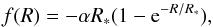 (2)obtained by fixing n = 1 in Eq. (1). We emphasize that γ gravity can satisfy all the stability and viability conditions. As discussed in O’Dwyer et al. (2013), for fixed n, there is a minimum value (αmin) of the parameter α such that for values α>αmin a late-time accelerated attractor is achieved. We consider this case throughout. From Eq. (1) we obtain the following derivatives:
  We note from Eq. (3) that with increasing n, the steepness of the f(R) function increases. Higher n means smaller | fR0 | , and the departures from GR will be smaller accordingly.
Although there is no cosmological constant, f(0) = 0, it follows from Eq. (1) that GR with Λ is recovered at high curvatures. Therefore, for R ≫ R∗ the models behave like ΛCDM. Since we are mainly interested in phenomena that occurred after the beginning of the matter-dominated era, we neglect radiation and write the effective cosmological constant (the cosmological constant of the reference ΛCDM model) as 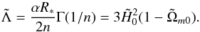 (5)In the equation above,
  denotes the present value of the matter density parameter that a ΛCDM model would have if it had the same matter density today (
 ) as the modified gravity f(R) model.
  represents the Hubble constant in the reference ΛCDM model. Therefore, we have
  , where Ωm0 and H0 are the present value of the matter energy density parameter and Hubble parameter in the f(R) model, respectively. It is useful to rewrite R∗ as
 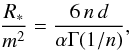 (6)where
  . To compute the background evolution, we start from the f(R) field equation for a FLRW metric
 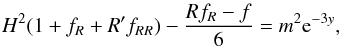 (7)where ′ ≡ d / dy (y = lna), H ≡ ȧ/a is the Hubble parameter (a dot denotes the derivative with respect to cosmic time), which is related to R by
  (8)To solve these equations, we introduce the new variables
 ![Mathematical equation: \begin{eqnarray} x_1 (y) &=& \frac{H^2}{m^2} - {\rm e}^{-3y} - d,\\[2mm] x_2 (y) &=& \frac{R}{m^2} - 3 {\rm e}^{-3y} - 12\left(d + x_1\right). \end{eqnarray}](/articles/aa/full_html/2016/03/aa27645-15/aa27645-15-eq56.png) With these definitions we obtain
With these definitions we obtain ![Mathematical equation: \begin{eqnarray} x'_1 (y) &=& \frac{x_2}{3},\\[2mm] x'_2 (y) &=& \frac{R'}{m^2} + 9 {\rm e}^{-3y} - 4 x_2, \end{eqnarray}](/articles/aa/full_html/2016/03/aa27645-15/aa27645-15-eq57.png) where R′ is given by Eq. (7). It is straightforward to verify that, as defined, x1 and x2 are always zero during the ΛCDM phase. We here focus on the three cases summarized in Table 1.
where R′ is given by Eq. (7). It is straightforward to verify that, as defined, x1 and x2 are always zero during the ΛCDM phase. We here focus on the three cases summarized in Table 1.
Furthermore, in terms of x1(y) and x2(y), the effective dark energy equation of state (wDE) is given by,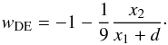 (13)For the considered models, the evolution of wDE as a function of the redshift z is shown in Fig. 1.
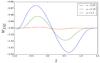 |
Fig. 1 Effective equation-of-state parameter wDE as a function of redshift z for the parameters given in Table 1. The strongest deviation from − 1 is lower than 4%. |
Overview of the model parameters for γ gravity.
For a general f(R) model the differential equation for the matter density contrast (δm) in the linear regime for subhorizon scales is given by (Pogosian & Silvestri 2008; Zhang 2006; de la Cruz-Dombriz et al. 2008)  (14)where
  (15)In GR, fRR = Q = 0, and there is no scale dependence for the density contrast in the linear regime. For ΛCDM the growing mode can be expressed in terms of hypergeometric function
  as (Silveira & Waga 1994)
 ![Mathematical equation: \begin{equation} \delta_+ \propto {\rm e}^{-y} {}_2 F_1 \left[ \frac{1}{3} , 1 , \frac{11}{6} , -{\rm e}^{3y}d \right]. \label{growth_lcdm} \end{equation}](/articles/aa/full_html/2016/03/aa27645-15/aa27645-15-eq74.png) (16)We solved Eq. (14) numerically and obtained the growing mode for the γ gravity. By using (16), we then obtained the fractional change in the matter power spectrum P(k) relative to ΛCDM. Figure 2 shows ΔPk/PΛ at z = 0 for the three choices of parameters shown in Table 1.
(16)We solved Eq. (14) numerically and obtained the growing mode for the γ gravity. By using (16), we then obtained the fractional change in the matter power spectrum P(k) relative to ΛCDM. Figure 2 shows ΔPk/PΛ at z = 0 for the three choices of parameters shown in Table 1.
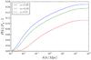 |
Fig. 2 Fractional difference in the matter power spectrum with respect to ΛCDM for different values of n and α, as indicated in Table 1. These results are used to compare with the nonlinear power spectrum from our numerical simulations. |
3. N-body equations
f(R)models are equivalent to a scalar-tensor theory (Brax et al. 2008), where the first derivative of the f(R) function, fR. This field propagates according the equation  (17)where κ2 = 8πG/c4 and T is the trace of energy-momentum tensor, T = gμνTμν. In the quasi-static limit (see, e.g., Noller et al. 2014; Bose et al. 2015; Llinares & Mota 2014, 2013) this equation becomes
  (18)where
  (19)and ΔR(a) = x2(a) + 12x1(a). The Ricci scalar R in function of fR is given by inverting Eq. (3)
 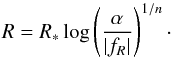 (20)The geodesic equation, needed to update the particle positions, reads
 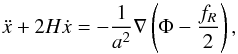 (21)where Φ is the Newtonian potential, which the dynamics is given by the Poisson equation
 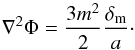 (22)When implementing these equations in the N-body code, we need to rewrite them in code-units given by
![Mathematical equation: \begin{eqnarray} &&\tilde{x} = x/B_0,~~~~ \tilde{\Phi} = \frac{\Phi a^2}{(H_0B_0)^2},\nonumber\\[2mm] &&{\rm d}\tilde{t} = \frac{H_0{\rm d}t}{a^2},~~~~\nabla_{\rm code} = B_0.\nabla. \end{eqnarray}](/articles/aa/full_html/2016/03/aa27645-15/aa27645-15-eq89.png) (23)Here B0 is the size of the simulation box. In terms of
(23)Here B0 is the size of the simulation box. In terms of  the evolution equations becomes
 ![Mathematical equation: \begin{eqnarray} \label{eq:alleq} &&\frac{{\rm d}^2\tilde{x}}{{\rm d}\tilde{t}^2} = -\nabla_{\rm code} \tilde{\Phi} - \frac{1}{2(B_0H_0)^2}\nabla_{\rm code} \tilde{f}_{R}, \\[2mm] &&\nabla_{\rm code}^2\tilde{\Phi} = \frac{3}{2}\Omega_{m0} a \delta_{\rm m}, \\[2mm] &&\nabla_{\rm code}^2 \tilde{f}_R = \Omega_{m0} (H_0B_0)^2 a^4 \\[2mm] &&\quad\quad\quad\times \left\{-\frac{R_*}{3m^2} \log\left(\frac{\alpha a^2}{\tilde{f}_R}\right)^{1/n} + \left[ a^{-3} + 4d + \frac{\Delta_R (a)}{3}\right] + a^{-3}\delta_{\rm m}\right\}\!.\nonumber \end{eqnarray}](/articles/aa/full_html/2016/03/aa27645-15/aa27645-15-eq92.png) These are the only equations we need to implement and solve in the N-body code.
These are the only equations we need to implement and solve in the N-body code.
For comparison we also need the linearized field equation. Simulations with this equation compared to the full fR equation is a good measure of the amount of screening that takes place in the model. The linearized fR equation is simply 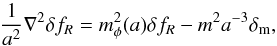 (27)where δfR = fR−fR(a) and
  . In code units, taking
  , we obtain
 ![Mathematical equation: \begin{eqnarray} \nabla_{\rm code}^2 u = [m_{\phi}(a)aB_0]^2 u + \delta_{\rm m} \frac{\Omega_{m0} a}{2}, \end{eqnarray}](/articles/aa/full_html/2016/03/aa27645-15/aa27645-15-eq97.png) (28)and the geodesic equation becomes
(28)and the geodesic equation becomes 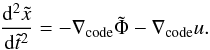 (29)We have
 ![Mathematical equation: \begin{eqnarray} m_{\phi}^2(a)a^2B_0^2 = \frac{a^2(H_0 B_0)^2}{3\alpha n}\frac{R(a)}{H_0^2} \left[\frac{R_*}{R(a)}\right]^n{\rm e}^{\left[R(a)/R_*\right]^n}. \end{eqnarray}](/articles/aa/full_html/2016/03/aa27645-15/aa27645-15-eq99.png) (30)
(30)
4. Implementation in the ISIS code
Implementing scalar-tensor theories of gravity in N-body code is rather straightforward because the scalar-tensor theories all contribute as a fifth force and because RAMSES, which ISIS is based on, has been widely used, thoroughly tested, and optimized. In this section we describe how the equations we need to solve are implemented in ISIS. For more details see Llinares et al. (2014).
To solve for fR directly is not numerically stable since the solution can potentially vary over several orders of magnitude when going from deep voids to massive clusters in our simulation. We therefore introduce a field redefinition | fR | = A(u) → ∇ | fR | = b(u)∇u where b(u) = dA(u) / du. The general field equation for fR discretized on a grid with the field-redefinition  , where u is the field we solve for, can be written as
 ![Mathematical equation: \begin{eqnarray} &&\mathcal{L}(u_{i,j,k}) = \nabla_{\rm code}\cdot [b(u)\nabla_{\rm code} u]_{i,j,k} + \Omega_{m0} (H_0B_0)^2 \\ &&\quad\times\left\{\frac{a^4 R_*}{3m^2} \log\left[\frac{\alpha a^2}{A(u_{i,j,k})}\right]^{1/n} - a(\delta_{\rm m})_{i,j,k} - a - a^4 \left[ 4d + \frac{\Delta_R (a)}{3} \right] \right\},\nonumber \end{eqnarray}](/articles/aa/full_html/2016/03/aa27645-15/aa27645-15-eq104.png) (31)where
(31)where ![Mathematical equation: \begin{eqnarray} &&\nabla_{\rm code}\cdot [b(u)\nabla_{\rm code} u]_{i,j,k} =\\ &&\quad\quad\qquad\frac{b_{i+1/2,j,k}(u_{i+1,j,k}-u_{i,j,k}) - b_{i-1/2,j,k}(u_{i,j,k}-u_{i-1,j,k})}{h^2}\nonumber\\ &&\quad\quad\qquad+\frac{b_{i,j+1/2,k}(u_{i,j+1,k}-u_{i,j,k}) - b_{i,j-1/2,k}(u_{i,j,k}-u_{i,j-1,k})}{h^2}\nonumber\\ &&\quad\quad\qquad+\frac{b_{i,j,k+1/2}(u_{i,j,k+1}-u_{i,j,k}) - b_{i,j,k-1/2}(u_{i,j,k}-u_{i,j,k-1})}{h^2},\nonumber \end{eqnarray}](/articles/aa/full_html/2016/03/aa27645-15/aa27645-15-eq105.png) (32)where h is the grid spacing and
(32)where h is the grid spacing and 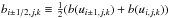 and where we have defined
  .
.
The equations are solved using Newton-Gauss-Seidel relaxation (with multigrid acceleration). The method consists of going through the grid and updating the solution using  (33)For this we also need ∂ℒ(ui,j,k) /∂ui,j,k, which is given by
 ![Mathematical equation: \begin{eqnarray} \frac{\partial\mathcal{L}(u_{i,j,k})}{\partial u_{i,j,k}} &= \frac{\partial \nabla_{\rm code}\cdot [b(u)\nabla_{\rm code} u]_{i,j,k}}{\partial u_{i,j,k}} \\&\quad - \Omega_{m0} (H_0B_0)^2\left\{\frac{a^4 R_*}{3m^2}\frac{b(u_{i,j,k})}{A(u_{i,j,k})} \log\left[\frac{\alpha}{A(u_{i,j,k})}\right]^{1/n-1}\right\},\nonumber \end{eqnarray}](/articles/aa/full_html/2016/03/aa27645-15/aa27645-15-eq111.png) (34)where
(34)where ![Mathematical equation: \begin{eqnarray} &&\frac{\partial \nabla_{\rm code}\cdot [b(u)\nabla_{\rm code} u]_{i,j,k}}{\partial u_{i,j,k}} = \\ &&\quad\qquad -\frac{b_{i+1/2,j,k} + b_{i-1/2,j,k}}{h^2} - \frac{b_{i,j+1/2,k} - b_{i,j-1/2,k}}{h^2} \nonumber\\ &&\quad\qquad-\frac{b_{i,j,k+1/2} + b_{i,j,k-1/2}}{h^2} + \frac{1}{2}c_{i,j,k}\left[\frac{u_{i+1,j,k} + u_{i-1,j,k} - 2u_{i,j,k}}{h^2} \right.\nonumber\\ &&\quad\qquad\left. + \frac{u_{i,j+1,k} + u_{i,j-1,k} - 2u_{i,j,k}}{h^2} + \frac{u_{i,j,k+1} + u_{i,j,k-1} -2u_{i,j,k}}{h^2}\right],\nonumber \end{eqnarray}](/articles/aa/full_html/2016/03/aa27645-15/aa27645-15-eq112.png) (35)and ci,j,k = c(ui,j,k), where
(35)and ci,j,k = c(ui,j,k), where  . Some problems arise related to how boundary conditions are handled on the refined grids in the code. This is discussed in Llinares et al. (2014) and Li et al. (2012b).
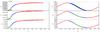 |
Fig. 3 Scalar field from tests. Different colors depict the different refinement levels. The left panel shows the field from a spherical density distribution, the right side shows a 1D sine field obtained in the second test. |
Our solver needs a starting guess, and for this we use the cosmological background solution, that is, the solution we would expect when there are no matter sources, ![Mathematical equation: \begin{eqnarray} |f_R(a)| = \alpha {\rm e}^{-\left[R(a)/R_*\right]^n} \to \overline{u} = A^{-1}(|f_R(a)|). \end{eqnarray}](/articles/aa/full_html/2016/03/aa27645-15/aa27645-15-eq116.png) (36)This is only needed when the simulation is stared as otherwise we can use the old solution as our guess. For γ gravity our choice for A and the related expressions for b are
(36)This is only needed when the simulation is stared as otherwise we can use the old solution as our guess. For γ gravity our choice for A and the related expressions for b are  and the background value of u is
 ![Mathematical equation: \begin{eqnarray} \overline{u} = A^{-1}(\tilde{f_R}(a)) = n\log\left[\frac{a^{-3} + 4d + \Delta_R (a) / 3}{R_*/(3H_0^2)}\right], \end{eqnarray}](/articles/aa/full_html/2016/03/aa27645-15/aa27645-15-eq120.png) (40)in terms of u we have
(40)in terms of u we have
![Mathematical equation: \begin{eqnarray} &&\mathcal{L}(u) = \nabla[b(u)\nabla u] + \Omega_{m0} (H_0B_0)^2 \\[2mm] &&\times\left[\frac{a^4 R_*}{3m^2} {\rm e}^{u/n} - a\delta_{\rm m} - a - a^3 \left(4d + \frac{\Delta_R (a)}{3} \right)\right], \nonumber\\[2mm] &&\frac{\partial}{\partial u} \mathcal{L}(u) = \frac{\partial}{\partial u}\nabla[b(u)\nabla u] + \Omega_{m0} (H_0 B_0)^2\left( \frac{a^4R_*}{3m^2} \frac{{\rm e}^{u/n}}{n} \right). \end{eqnarray}](/articles/aa/full_html/2016/03/aa27645-15/aa27645-15-eq121.png) When the fifth force is implemented, we simply replace it with an effective force Feff that includes the effects of modified gravity wherever the code normally works with the gravitational force, FN,
When the fifth force is implemented, we simply replace it with an effective force Feff that includes the effects of modified gravity wherever the code normally works with the gravitational force, FN,  (43)The expression for the fifth force in code-units is given in Eq. (24), and we use the same five-point stencil as RAMSES uses to compute the gravitational force
  to compute the fifth force
  .
.
5. Tests of the N-body solver
To verify that the solver is implemented correctly, we tested it several times. We present some of these tests in this section. The density is provided to the code through a distribution of particles. The density estimation (CIC) and refinement criteria are the same as those used for the cosmological simulations. We also have the option to set the density field analytically in the code. To test that the treatment of the boundary of the refinement is correct, we included two levels of refinement. The model parameters used for the tests are the same as mentioned previously in Table 1.
The first test case corresponds to a sphere of radius R of constant density located in the center of the box and embedded in a uniform background:  (44)where
  characterizes the density contrast between the inside and outside of the sphere,
  is the mean density, R is the radius of the sphere, and B0 the size of the box. The value of δ chosen for the test is 5000. For the f(R) test we used R = 25 Mpc/h and B0 = 250 Mpc/h. A spherical symmetric configuration is effectively one-dimensional, therefore the field equation reduces to an ODE, which we solved by using Mathematica and used this to compare with.
For the second test we analytically computed a density field ρ(x,y,z) ≡ ρ(x) (i.e., a 1D configuration), using the field equation, so that the solution is given by a sine: u ∝ 2 + sin(2πx).
Figure 3 shows the result of both these tests and the different colors depict the different refinement levels. We see that the curves are smooth when going from one level to another, which demonstrates that boundary conditions are handled properly. The tests were performed using the serial version of the code, and both tests give the expected results, which demonstrates that the code works properly.
6. Simulations
The γ gravity simulations were run using 5123 dark matter particles with a box size of B0 = 250 Mpc/h, and we refined cells whenever it had more than eight particles in it. The highest refinement level reached in our simulation was eight. The background cosmology used for the simulation was computed using Eq. (7) with h = 0.71, ΩΛ = 0.733 and Ωm0 = 0.267.
The model parameters were presented in Sect. 2, with some plots of various background quantities. We also compared these simulations with simulations of the Hu-Sawicki f(R) model from Llinares et al. (2014).
7. Results
7.1. Power spectrum
The nonlinear matter power spectrum is an important observable and could be used to distinguish among different models of structure formation. As we showed above, γ gravity can have a strong effect on the growth rate of the linear perturbations. We expect these signatures to be detectable in the nonlinear matter power spectrum.
To compute the power spectrum we used a public code, POWMES (Colombi & Novikov 2011), which uses folding methods to compute the power spectrum.
Figure 4 displays the difference of the matter power spectrum with respect to ΛCDM, defined as ΔP/PΛCDM ≡ P(k) /PΛCDM(k)−1 for γ gravity together with the corresponding predictions from linear perturbations theory and the Hu-Sawicki f(R) model for comparison. We focus on the present-day epoch, which corresponds to z = 0.
Figure 4 shows that the differences from ΛCDM are lower than 5−10% for all of our runs in the range 0.05 h Mpc-1 ≲ k ≲ 0.1 h Mpc-1 and in agreement with the linear perturbation result seen in Fig. 2. The deviation from ΛCDM approaches zero for larger scales. This is because the range of fifth force is smaller than the horizon, therefore the modifications of gravity are not felt on the largest scales. On smaller, nonlinear scales, the full effect of the fifth force acts, and we see larger deviations. However, ΔP/PΛCDM continues to grow with k in γ gravity, in contrast to the Hu-Sawicky model, where the chameleon screening mechanism is in play on these scales, which reduces the power enhancement. This is an indication that the screening mechanism does not work very well in our simulation. We discuss this in more detail in Sect. 7.4.
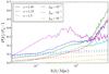 |
Fig. 4 Fractional deviation of the dark matter power spectrum with respect to the ΛCDM model. The linear predictions of γ gravity are represented by dashed lines. For comparison we also show the results from simulations with the Hu-Sawicky f(R) model with | fR0 | = { 10-4,10-5,10-6 } from Llinares et al. (2014). |
7.2. Halo mass function
The halo mass function, the number density of halos with a given mass, is a useful tool for investigating the efficiency of a model in forming halos of different masses. To locate halos in the simulation outputs, we used the AHF (Amiga Halo Finder, Knollmann & Knebe 2009). We determined the halo mass function by binning halos in logarithmic mass intervals.
In Fig. 5 we show the fractional difference with respect to ΛCDM of halo mass function computed from our simulations. Our measurement of the halo mass function itself is limited by statistics and to a lesser extent, by the resolution in the high and low mass end. However, we can reduce the impact of these two effects by considering the relative difference between the halo mass functions measured in modified gravity and ΛCDM simulations with the same initial condition.
Figure 5 shows that we find an excess of halos in the range 1013 ≲ M/M⊙ ≲ 1015 probed by our simulation in γ gravity, and the signatures are very similar to the | fR0 | ≳ 10-5 Hu-Sawicki model. For the most massive halos (M/M⊙ ≳ 1015) the effect of screening is much more pronounced in Hu-Sawicki models, and the mass-function approaches ΛCDM. This does not occur for γ gravity and is again an indication that the chameleon screening mechanism does not work very efficiently in our simulations.
For γ gravity, the number of halos increases significantly, especially at the high mass end, by up to 40−100% for cluster-sized halos. For Hu-Sawicki models, when the value of the fR field becomes comparable to the cosmological potential wells, the chameleon effect starts to operate. This can be seen in the mass function, where deviations from ΛCDM approach zero in the high- mass end for models with | fR0 | = 10-5 and | fR0 | = 10-6.
The large deviations we find Δn/nΛCDM ~ 0.5−1 in the high-mass end are probably already ruled out by present cluster counts (Cataneo et al. 2015; Mak et al. 2012). This does not rule out the model per se, but requires choices of parameters where | fR0 | is much smaller today, leading to no signatures in the background evolution (i.e., in the Hubble factor) of the Universe.
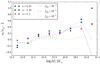 |
Fig. 5 Fractional difference of the halo mass function for γ gravity (data points) with respect to the ΛCDM model. For comparison we also show the results from simulations with the Hu-Sawicky f(R) model with | fR0 | = { 10-4,10-5,10-6 } (dashed lines) from Llinares et al. (2014). |
7.3. Halo profiles
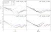 |
Fig. 6 Fractional difference in the halo density profiles with respect to ΛCDM for four different mass bins. For comparison we also show the results from simulations with the Hu-Sawicky f(R) model with | fR0 | = { 10-4,10-5,10-6 } (dashed lines) from Llinares et al. (2014). |
We also studied how modifications of gravity change the density and velocity profiles of dark matter halos. We focused on halos in the mass ranges 0.5−1 × 10¹³ Mpc/h, 1−5 × 10¹³ Mpc/h, 0.5−1 × 10¹⁴ Mpc/h, and 1−5 × 10¹⁴ Mpc/h. The density profiles were calculated by binning dark matter particles in annular bins for each halo. Our calculated density profiles are averages of all density profiles of the proper size, ranging from 10% of the virialization radius, r = 0.1Rvir, to ten times the virialization radius, r = 10Rvir. This range was chosen to properly include all behaviors of the fifth force on the dark matter halos while also avoiding the inner regions of the halos, where the resolution of our simulations is not sufficient.
Figure 6 shows the fractional difference with respect to ΛCDM in the density profiles. We first note that the inner regions (R<Rvir) of halos for γ gravity are significantly denser than in ΛCDM. This difference is compensated for in outer regions (R>Rvir). Moreover, the profiles between the different model parameters do not differ appreciably from each other, and this pattern repeats for all ranges. However, the density profiles for Hu-Sawicki models in general show stronger clustering in the low-density regions in the outskirts of halos than in the inner regions.
In the velocities profiles, shown in Fig. 7, we expect the fifth force to increase the velocity dispersion. This effect is very similar for both models, except for most massive halos, for which the Hu-Sawicki models are more screened, causing a substantial decrease in comparison to γ gravity. For the Hu-Sawicki model the velocities are boosted by ~20% in the | fR0 | = 10-4 case and by 5% in the | fR0 | = 10-6 case for all the three halo mass ranges analyzed. Only for the | fR0 | = 10-5 parameters a mixed behavior is seen, that is, for the lower two halo mass ranges the boost is ~20%, but for the heaviest halos there is no deviation from ΛCDM in the inner parts and ~15% higher velocities are found in the outer parts. For γ gravity, the difference between the models we simulated is more expressive for less massive halos (5 × 10¹²<M/M⊙< 1013 and 1013<M/M⊙< 5 × 10¹³), for most massive halos (1014<M/M⊙< 5 × 10¹⁴) only the case α = 1.5 is distinguishable from the others.
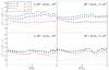 |
Fig. 7 Fractional difference in the velocity dispersion profiles with respect to ΛCDM for four different mass bins. For comparison we also show the results from simulations with the Hu-Sawicky f(R) model with | fR0 | = { 10-4,10-5,10-6 } (dashed lines) from Llinares et al. (2014). |
7.4. Fifth force and screening
General relativity is very well tested on very small scales, especially inside the solar system. To ensure that Fφ is not relevant at these scales, we need a screening mechanism to suppress the fifth force at small-scale, very high curvature regimes.
When γ gravity was proposed in O’Dwyer et al. (2013), the authors explored the compatibility between the model and the solar system experiments using the chameleon mechanism for screening, as any other f(R) (Brax et al. 2008).
As we showed in the results above, the screening mechanism does not seem to be working very efficiently for the models simulated here. To check how much the fifth force is screened in our simulations, we compared the magnitude of the fifth and Newtonian force on the particles in our simulation box, as in Davis et al. (2012).
Figure 8 shows a scatter plot for this comparison at redshift z = 0. The dispersion for small FN< 0.01 is expected (numerical scatter), here the forces are tiny, so the scatter here has a very weak effect on the simulation. The important part in this figure is the behavior for large FN. If we have screening, then we should see Fφ ≪ FN/ 3 in high-density regions (which corresponds to high values of FN). The result we find shows that the force ratio is roughly onethird – which is the linear prediction – everywhere, meaning that there is very little screening present in our simulations.
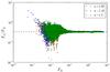 |
Fig. 8 Comparison between the magnitudes of Newtonian force (FN) and fifth force (Fφ), the dashed line indicates FN/Fφ = 1 / 3. The forces are in units of H0/c2. |
To understand this better, we revisit the screening conditions. Considering a spherical symmetric body with constant density ρc embedded in the background of constant density ρb, the solutions to the field equation (see e.g. Brax et al. 2012) mean that the fifth force is given by 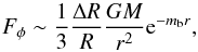 where
where 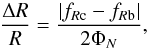 is the so-called screening factor (also called the thin-shell) and fRb (fRc) is the value of fR in the background (inside the body), where ρ = ρb (ρc). If
  the fifth force is screened and we recover General Relativity. If
  we instead find that
  and gravity is significantly modified.
When the field is located in the minimum of its effective potential in the background2, we can calculate the screening factor analytically. Assuming this, we find that for the γ gravity models considered here, Earth and Sun are almost completely screened and pass local gravity constraints assuming the galaxy is screened.
However, for the parameter values considered in this paper, the screening condition gives that the galaxy is not screened which again implies that the Earth and the sun is not screened either3. The only caveat to this is that screening might have survived from earlier times. At early redshift  and almost all objects are screened. Then in the cosmological evolution
  very quickly evolves to high values
  . The field inside our galaxy might have been trapped, ensuring screening. This is not expected, but to rigorously rule out (or confirm) this possibility, we would need simulations beyond the quasi-static approximation that we assumed in our simulations. This is beyond the scope of this paper.
8. Summary and conclusions
We have investigated the nonlinear evolution in γ gravity, a f(R) theory of gravity that is a viable alternative to ΛCDM. The models we investigated use a screening mechanism to suppress the deviations from General Relativity at small (solar system) and large cosmological scales. Specifically, this is the chameleon screening mechanism. As a result of this screening mechanism, the strongest signatures in these models are expected to occur at the nonlinear regime of structure formation. Therefore, to unveil the imprints of such theories at astrophysical scales, we ran several cosmological N-body simulations. We compared models with ΛCDM and the Hu-Sawicki model and showed that several astrophysical observables (halo mass function, density profiles, and power spectra) show the signatures of the model significantly strongly.
For the matter power spectrum we found a small deviation, lower than 10%, on large scales (k ≲ 10-1h/Mpc), which is consistent with the predictions of linear perturbation theory. For small scales (k ≳ 10-1h/Mpc), on the other hand, we found a strong increase in power, the largest deviation (α = 1.18) reaches ~60%, and in the other cases (α = 1.05 and α = 1.5) it reaches ~50%. This is quite different from the results found in the Hu-Sawicky model, where the screening of the fifth force is much more active in suppressing the enhancement of power on small scales, the largest deviation is ~30%, much lower than for γ gravity.
For the halo mass function we found that all of our runs gave very similar result in the mass range 11.5 < log (M/M⊙) < 14.7, and these results are very similar to what is found in the Hu-Sawicky model for | fR0 | ≥ 10-5; a 10−60% increase in the halo abundance. However, for γ gravity we found an enhancement of 40−100% in the abundance for log (M/M⊙) > 14.5, which can be compared to the Hu-Sawicki model, where the halo mass function approaches that of ΛCDM.
For halo density profiles we found that the different runs with γ gravity were not distinguished well in any mass range; in all situations we saw that the inner regions (R < Rvir) of halos for γ gravity are significantly thicker than the halos of ΛCDM, around 10% for less massive halos, 5 × 10¹² < M/M⊙ < 1013, increasing with the halo mass until they reached ~30% for the most massive halos, 1014 <M/M⊙ < 5 × 10¹⁴. This difference is compensated for in the outer regions (R > Rvir). For the Hu-Sawicki model the same effect acts for less massive halos 5 × 10¹² <M/M⊙ < 1013, but it changes for more massive halos, 5 × 10¹³ < M/M⊙ < 1014 and 1014 < M/M⊙ < 5 × 10¹⁴ when the screening mechanism suppresses the fifth force. This then leads to a suppression in the accretion of mass concentration in the inner regions (compared to the non-screened case).
Finally, we computed the velocity profiles, and as we expected, the velocities are significantly enhanced in γ gravity compared to ΛCDM. The other cases are comparable in all mass ranges, but with some important signatures. The difference between the different γ gravity models is larger for low-mass halos, 5 × 10¹² < M/M⊙ < 1013, and we can distinguish them from each other; the differences reach ~30% close to the boundary region, R ~ Rvir. This difference decreases with the mass of the halos, and for the most massive halos 1014 < M/M⊙ < 5 × 10¹⁴. Only the case α = 1.5 is lower than ~10% from the others, which are practically identical.
The chameleon mechanism – the screening mechanism that makes f(R) gravity viable – is not very effective for the parameter choices considered in this paper. This explains the large deviations from ΛCDM in the observables we considered. Especially the cluster count signatures of 40−100% in the high-mass end M ≳ 1014.5M⊙ disagree with current observations. This does not rule out the model per se, but require choices of parameters where | fR0 | is much smaller today, which implies that the model has no observable signatures in the background evolution (i.e., in the Hubble factor) of the Universe.
With observable signatures we mean that the equation of state differs enough from the ΛCDM value of w = −1 at low redshifts that such a deviation could be detected by near-future experiments like WFIRST (Spergel et al. 2015), for example.
Background here refers to the surroundings for the body in question, not necessarily the cosmological background.
This is only true for the parameters considered in this paper. If | fR0 | ≲ 10-5, then the galaxy, Earth, and our Sun are screened.
Acknowledgments
M.V.S. thanks the Brazilian research agency CAPES and the University of Oslo for support and Max B. Grönke and Amir Hammami for useful discussions. H.A.W. is supported by BIPAC and the Oxford Martin School. D.F.M. would like to thank the Research Council of Norway for funding. The simulations were performed on the NOTUR cluster HEXAGON, which is the computing facility at the University of Bergen.
References
- Amendola, L., Gannouji, R., Polarski, D., & Tsujikawa, S. 2007, Phys. Rev. D, 75, 083504 [NASA ADS] [CrossRef] [Google Scholar]
- Appleby, S. A., & Battye, R. A. 2007, Phys. Lett. B, 654, 7 [NASA ADS] [CrossRef] [MathSciNet] [Google Scholar]
- Appleby, S. A., Battye, R. A., & Starobinsky, A. A. 2010, J. Cosmol. Astropart. Phys., 1006, 005 [NASA ADS] [CrossRef] [Google Scholar]
- Berti, E., Barausse, E., Cardoso, V., et al. 2015, Class. Quant. Grav. 32, 243001 [Google Scholar]
- Boehmer, C. G., Burnett, J., Mota, D. F., & Shaw, D. J. 2010, J. High Energy Phys., 07, 053 [NASA ADS] [CrossRef] [Google Scholar]
- Bose, S., Hellwing, W. A., & Li, B. 2015, J. Cosmol. Astropart. Phys., 2, 34 [Google Scholar]
- Brax, P., van de Bruck, C., Davis, A.-C., & Shaw, D. J. 2008, Phys. Rev. D, 78, 104021 [NASA ADS] [CrossRef] [MathSciNet] [Google Scholar]
- Brax, P., Davis, A.-C., Li, B., & Winther, H. A. 2012, Phys. Rev. D, 86, 044015 [NASA ADS] [CrossRef] [Google Scholar]
- Brax, P., Davis, A.-C., Li, B., Winther, H. A., & Zhao, G.-B. 2013, J. Cosmol. Astropart. Phys., 4, 29 [Google Scholar]
- Cai, Y.-C., Padilla, N., & Li, B. 2015, MNRAS, 451, 1036 [NASA ADS] [CrossRef] [Google Scholar]
- Capozziello, S., Cardone, V. F., Carloni, S., & Troisi, A. 2003, Int. J. Mod. Phys. D, 12, 1969 [Google Scholar]
- Carroll, S. M., Duvvuri, V., Trodden, M., & Turner, M. S. 2004, Phys. Rev. D, 70, 043528 [NASA ADS] [CrossRef] [Google Scholar]
- Cataneo, M., Rapetti, D., Schmidt, F., et al. 2015, Phys. Rev. D, 92, 044009 [NASA ADS] [CrossRef] [Google Scholar]
- Cognola, G., Elizalde, E., Nojiri, S., et al. 2008, Phys. Rev. D, 77, 046009 [NASA ADS] [CrossRef] [Google Scholar]
- Colombi, S., & Novikov, D. 2011, Astrophysics Source Code Library [record ascl:1110.017] [Google Scholar]
- Davis, A.-C., Li, B., Mota, D. F., & Winther, H. A. 2012, ApJ, 748, 61 [NASA ADS] [CrossRef] [Google Scholar]
- de la Cruz-Dombriz, A., Dobado, A., & Maroto, A. L. 2008, Phys. Rev. D, 77, 123515 [NASA ADS] [CrossRef] [Google Scholar]
- Frolov, A. V. 2008, Phys. Rev. Lett., 101, 061103 [NASA ADS] [CrossRef] [MathSciNet] [PubMed] [Google Scholar]
- Gronke, M., Llinares, C., Mota, D. F., & Winther, H. A. 2015, MNRAS, 449, 2837 [NASA ADS] [CrossRef] [Google Scholar]
- Hammami, A., Llinares, C., Mota, D. F., & Winther, H. A. 2015, MNRAS, 449, 3635 [NASA ADS] [CrossRef] [Google Scholar]
- He, J.-h., Li, B., & Jing, Y. P. 2013, Phys. Rev. D, 88, 103507 [NASA ADS] [CrossRef] [Google Scholar]
- He, J.-h., Li, B., & Hawken, A. J. 2015, Phys. Rev. D, 92, 103508 [NASA ADS] [CrossRef] [Google Scholar]
- Hellwing, W. A., Cautun, M., Knebe, A., Juszkiewicz, R., & Knollmann, S. 2013, J. Cosmol. Astropart. Phys., 1310, 012 [Google Scholar]
- Hellwing, W. A., Barreira, A., Frenk, C. S., Li, B., & Cole, S. 2014, Phys. Rev. Lett., 112, 221102 [NASA ADS] [CrossRef] [Google Scholar]
- Hu, W., & Sawicki, I. 2007, Phys. Rev. D, 76, 064004 [CrossRef] [Google Scholar]
- Jain, B., & Khoury, J. 2010, Annals Phys., 325, 1479 [Google Scholar]
- Knollmann, S. R., & Knebe, A. 2009, ApJS, 182, 608 [NASA ADS] [CrossRef] [Google Scholar]
- Li, B., Mota, D. F., & Barrow, J. D. 2011, ApJ, 728, 109 [NASA ADS] [CrossRef] [Google Scholar]
- Li, B., Zhao, G.-B., Teyssier, R., & Koyama, K. 2012a, J. Cosmol. Astropart. Phys., 1, 51 [Google Scholar]
- Li, B., Zhao, G.-B., Teyssier, R., & Koyama, K. 2012b, J. Cosmol. Astropart. Phys., 1201, 051 [Google Scholar]
- Li, B., Hellwing, W. A., Koyama, K., et al. 2013, MNRAS, 428, 743 [NASA ADS] [CrossRef] [Google Scholar]
- Linder, E. V. 2009, Phys. Rev. D, 80, 123528 [NASA ADS] [CrossRef] [Google Scholar]
- Llinares, C., & Mota, D. 2013, Phys. Rev. Lett., 110, 161101 [NASA ADS] [CrossRef] [Google Scholar]
- Llinares, C., & Mota, D. F. 2014, Phys. Rev. D, 89, 084023 [NASA ADS] [CrossRef] [Google Scholar]
- Llinares, C., Mota, D. F., & Winther, H. A. 2014, A&A, 562, A78 [NASA ADS] [CrossRef] [EDP Sciences] [Google Scholar]
- Lombriser, L., Schmidt, F., Baldauf, T., et al. 2012, Phys. Rev. D, 85, 102001 [NASA ADS] [CrossRef] [Google Scholar]
- Lombriser, L., Koyama, K., & Li, B. 2014, J. Cosmol. Astropart. Phys., 1403, 021 [NASA ADS] [CrossRef] [Google Scholar]
- Mak, D. S. Y., Pierpaoli, E., Schmidt, F., & Macellari, N. 2012, Phys. Rev. D, 85, 123513 [NASA ADS] [CrossRef] [Google Scholar]
- Mota, D. F., Shaw, D. J., & Silk, J. 2008, ApJ, 675, 29 [NASA ADS] [CrossRef] [Google Scholar]
- Noller, J., von Braun-Bates, F., & Ferreira, P. G. 2014, Phys. Rev. D, 89, 023521 [NASA ADS] [CrossRef] [Google Scholar]
- O’Dwyer, M., Joras, S. E., & Waga, I. 2013, Phys. Rev. D, 88, 063520 [NASA ADS] [CrossRef] [Google Scholar]
- Oyaizu, H., Lima, M., & Hu, W. 2008, Phys. Rev. D, 78, 123524 [NASA ADS] [CrossRef] [Google Scholar]
- Perlmutter, S., Aldering, G., Goldhaber, G., et al. 1999, ApJ, 517, 565 [NASA ADS] [CrossRef] [Google Scholar]
- Pogosian, L., & Silvestri, A. 2008, Phys. Rev. D, 77, 023503; Erratum: 2010, 81, 049901 [NASA ADS] [CrossRef] [Google Scholar]
- Planck Collaboration XXII. 2014, A&A, 571, A22 [NASA ADS] [CrossRef] [EDP Sciences] [Google Scholar]
- Puchwein, E., Baldi, M., & Springel, V. 2013, MNRAS, 436, 348 [NASA ADS] [CrossRef] [Google Scholar]
- Pujol, A., Gaztañaga, E., Giocoli, C., et al. 2014, MNRAS, 438, 3205 [NASA ADS] [CrossRef] [Google Scholar]
- Riess, A. G., Filippenko, A. V., Challis, P., et al. 1998, AJ, 116, 1009 [NASA ADS] [CrossRef] [Google Scholar]
- Schmidt, F. 2010, Phys. Rev. D, 81, 103002 [NASA ADS] [CrossRef] [Google Scholar]
- Schmidt, F., Lima, M. V., Oyaizu, H., & Hu, W. 2009, Phys. Rev. D, 79, 083518 [NASA ADS] [CrossRef] [Google Scholar]
- Shi, D., Li, B., Han, J., Gao, L., & Hellwing, W. A. 2015, MNRAS, 452, 3179 [NASA ADS] [CrossRef] [Google Scholar]
- Silveira, V., & Waga, I. 1994, Phys. Rev. D, 50, 4890 [NASA ADS] [CrossRef] [Google Scholar]
- Song, Y.-S., Taruya, A., Linder, E., et al. 2015, Phys. Rev. D, 92, 043522 [NASA ADS] [CrossRef] [Google Scholar]
- Spergel, D., Gehrels, N., Baltay, C., et al. 2015, ArXiv e-prints [arXiv:1503.03757] [Google Scholar]
- Starobinsky, A. A. 1980, Phys. Lett. B, 91, 99 [NASA ADS] [CrossRef] [Google Scholar]
- Starobinsky, A. A. 2007, JETP Lett., 86, 157 [NASA ADS] [CrossRef] [Google Scholar]
- Terukina, A., & Yamamoto, K. 2012, Phys. Rev. D, 86, 103503 [NASA ADS] [CrossRef] [Google Scholar]
- Tessore, N., Winther, H. A., Metcalf, R. B., Ferreira, P. G., & Giocoli, C. 2015, J. Cosmol. Astropart. Phys., 10, 36 [Google Scholar]
- Teyssier, R. 2002, A&A, 385, 337 [NASA ADS] [CrossRef] [EDP Sciences] [Google Scholar]
- Thongkool, I., Sami, M., Gannouji, R., & Jhingan, S. 2009, Phys. Rev. D, 80, 043523 [NASA ADS] [CrossRef] [Google Scholar]
- Wilcox, H., Bacon, D., Nichol, R. C., et al. 2015, MNRAS, 452, 1171 [NASA ADS] [CrossRef] [Google Scholar]
- Winther, H. A., Mota, D. F., & Li, B. 2012, ApJ, 756, 166 [NASA ADS] [CrossRef] [Google Scholar]
- Winther, H. A., Schmidt, F., Barreira, A., et al. 2015, MNRAS, 454, 4208 [NASA ADS] [CrossRef] [Google Scholar]
- Zhang, P. 2006, Phys. Rev. D, 73, 123504 [NASA ADS] [CrossRef] [Google Scholar]
- Zhao, G.-B., Li, B., & Koyama, K. 2011, Phys. Rev. D, 83, 044007 [NASA ADS] [CrossRef] [Google Scholar]
- Zivick, P., Sutter, P. M., Wandelt, B. D., Li, B., & Lam, T. Y. 2015, MNRAS, 451, 4215 [NASA ADS] [CrossRef] [Google Scholar]
- Zumalacarregui, M., Koivisto, T. S., & Mota, D. F. 2013, Phys. Rev. D, 87, 083010 [NASA ADS] [CrossRef] [Google Scholar]
All Tables
All Figures
|
Fig. 1 Effective equation-of-state parameter wDE as a function of redshift z for the parameters given in Table 1. The strongest deviation from − 1 is lower than 4%. |
| In the text | |
|
Fig. 2 Fractional difference in the matter power spectrum with respect to ΛCDM for different values of n and α, as indicated in Table 1. These results are used to compare with the nonlinear power spectrum from our numerical simulations. |
| In the text | |
|
Fig. 3 Scalar field from tests. Different colors depict the different refinement levels. The left panel shows the field from a spherical density distribution, the right side shows a 1D sine field obtained in the second test. |
| In the text | |
|
Fig. 4 Fractional deviation of the dark matter power spectrum with respect to the ΛCDM model. The linear predictions of γ gravity are represented by dashed lines. For comparison we also show the results from simulations with the Hu-Sawicky f(R) model with | fR0 | = { 10-4,10-5,10-6 } from Llinares et al. (2014). |
| In the text | |
|
Fig. 5 Fractional difference of the halo mass function for γ gravity (data points) with respect to the ΛCDM model. For comparison we also show the results from simulations with the Hu-Sawicky f(R) model with | fR0 | = { 10-4,10-5,10-6 } (dashed lines) from Llinares et al. (2014). |
| In the text | |
|
Fig. 6 Fractional difference in the halo density profiles with respect to ΛCDM for four different mass bins. For comparison we also show the results from simulations with the Hu-Sawicky f(R) model with | fR0 | = { 10-4,10-5,10-6 } (dashed lines) from Llinares et al. (2014). |
| In the text | |
|
Fig. 7 Fractional difference in the velocity dispersion profiles with respect to ΛCDM for four different mass bins. For comparison we also show the results from simulations with the Hu-Sawicky f(R) model with | fR0 | = { 10-4,10-5,10-6 } (dashed lines) from Llinares et al. (2014). |
| In the text | |
|
Fig. 8 Comparison between the magnitudes of Newtonian force (FN) and fifth force (Fφ), the dashed line indicates FN/Fφ = 1 / 3. The forces are in units of H0/c2. |
| In the text | |
Current usage metrics show cumulative count of Article Views (full-text article views including HTML views, PDF and ePub downloads, according to the available data) and Abstracts Views on Vision4Press platform.
Data correspond to usage on the plateform after 2015. The current usage metrics is available 48-96 hours after online publication and is updated daily on week days.
Initial download of the metrics may take a while.