| Issue |
A&A
Volume 587, March 2016
|
|
|---|---|---|
| Article Number | A65 | |
| Number of page(s) | 8 | |
| Section | The Sun | |
| DOI | https://doi.org/10.1051/0004-6361/201527530 | |
| Published online | 17 February 2016 | |
The IAG solar flux atlas: Accurate wavelengths and absolute convective blueshift in standard solar spectra⋆
Georg-August Universität Göttingen, Institut für Astrophysik, Friedrich-Hund-Platz 1, 37077 Göttingen, Germany
e-mail: This email address is being protected from spambots. You need JavaScript enabled to view it.
Received: 9 October 2015
Accepted: 8 November 2015
Abstract
We present a new solar flux atlas with the aim of understanding wavelength precision and accuracy in solar benchmark data. The atlas covers the wavelength range 405−2300 nm and was observed at the Institut für Astrophysik, Göttingen (IAG), with a Fourier transform spectrograph (FTS). In contrast to other FTS atlases, the entire visible wavelength range was observed simultaneously using only one spectrograph setting. We compare the wavelength solution of the new atlas to the Kitt Peak solar flux atlases and to the HARPS frequency-comb calibrated solar atlas. Comparison reveals systematics in the two Kitt Peak FTS atlases resulting from their wavelength scale construction, and shows consistency between the IAG and the HARPS atlas. We conclude that the IAG atlas is precise and accurate on the order of ± 10 m s-1 in the wavelength range 405−1065 nm, while the Kitt Peak atlases show deviations as large as several ten to 100 m s-1. We determine absolute convective blueshift across the spectrum from the IAG atlas and report slight differences relative to results from the Kitt Peak atlas that we attribute to the differences between wavelength scales. We conclude that benchmark solar data with accurate wavelength solution are crucial to better understand the effect of convection on stellar radial velocity measurements, which is one of the main limitations of Doppler spectroscopy at m s -1 precision.
Key words: atlases / line: identification / methods: observational / standards / Sun: fundamental parameters
Data (FITS files of the spectra) and Table A.1 are only available at the CDS via anonymous ftp to cdsarc.u-strasbg.fr (130.79.128.5) or via http://cdsarc.u-strasbg.fr/viz-bin/qcat?J/A+A/587/A65
© ESO, 2016
1. Introduction
High-resolution spectra of the Sun are important benchmarks for various astrophysical fields. The high quality in spectral resolution and signal-to-noise ratio (S/N) allows investigation of fundamental processes in atomic and molecular physics, the structure of the solar atmosphere, and the subtleties of line formation including convective motion (see, e.g., Dravins 1982). The last is particularly important for our understanding of stellar spectra (e.g., Gray 2009), for which observations of the Sun as a star − solar flux observations − are required. Another important field for solar benchmark data is the growing interest in ultra-high-precision radial velocity (RV) observations (m s-1 and even cm s-1 precision) for which stellar convection becomes relevant as a fundamental limit (Saar & Donahue 1997; Meunier & Lagrange 2013; Dumusque et al. 2014). Reaching out to m s-1 Doppler precision and below requires that the wavelength scale of solar benchmark data be precise and accurate at that level. While precision is enough when data taken with the same instrument and the same star are analyzed, for example, for RV of one star, a comparison between data from other stars and solar data taken with different instruments and from different parts of the Sun (full disk, disk center, spot, etc.) requires an understanding of the accuracy of the wavelength scales. In this paper, we present a new high-fidelity atlas of the solar flux and analyze precision and accuracy of standard solar atlases.
A comprehensive overview of the line asymmetries and wavelength shifts in solar and stellar data was provided by Dravins (2008). His Fig. 5 shows the remarkable difference of a few 100 m s-1 between Ti ii bisectors when calculated from different solar disk center spectra. We focus on solar flux atlases, i.e., spectra taken from the entire solar disk or the Sun observed as a star that can be used to compare stellar to solar observations. The most commonly used solar flux atlas is the Kitt Peak atlas by Kurucz et al. (1984) observed at McMath National Solar Observatory with a Fourier transform spectrograph (FTS). Another flux atlas from this facility was published in Wallace et al. (2011). It is often assumed that the FTS atlases provide high wavelength accuracy, but this is not necessarily the case at a level of a few tens of m s-1. In this paper, we carry out a detailed comparison between the two Kitt Peak FTS atlases and the new atlas presented here. As a third benchmark, we include the solar flux atlas from Molaro et al. (2013) observed with HARPS and wavelength calibrated with a laser frequency comb (LFC). While the spectral fidelity of this atlas is not as high as in the FTS atlases (because of lower instrumental resolution) and the wavelength coverage is limited, the wavelength solution is presumably the most accurate currently available.
FTS settings used for the two solar atlases.
The accuracy that can be reached in the wavelength calibration of solar atlases is a crucial factor for the future development of high-precision RV surveys. At the 1 m s-1 level, we observe the influence of stellar convection and activity, and stellar RV surveys can be fooled or at least hampered by the presence of regular changes in stellar convective patterns. One of the most challenging tasks today for our understanding (and correction) of Doppler shifts from convective patterns is the effect of suppressed convective blueshift in active regions (Dravins et al. 1981). Dumusque et al. (2014) provided a tool for simulating the influence of activity on stellar RV measurements. Useful templates for this task are FTS measurements from the solar disk and solar spots. However, the results from such a simulation need to be interpreted with care because the absolute wavelength scales of the template spectra are not understood to the level required for precision RV work. It is the purpose of this paper to investigate the typical wavelength uncertainties of the available standard solar atlases, and to identify the challenges we have to overcome in order to provide useful input for future RV simulations.
The paper consists of three parts. First, we describe our new FTS atlas and the other atlases used for comparison in Sects. 2−4. Second, we compare the wavelength solutions of the atlases among each other in Sect. 5. Finally, we use our new atlas in Sect. 6 to re-investigate convective blueshift in the solar flux spectrum, and we provide absolute values for convective blueshift as a function of line depth.
2. The instrument
At the Institut für Astrophysik, Göttingen (IAG), we are operating a Fourier transform spectrograph (FTS) Bruker IFS 125 HR with a maximum optical path length of 228 cm in asymmetric mode (50 cm in symmetric mode), resulting in a maximum resolving power exceeding R = 106 for wavelengths shorter than 2 μm, but the resolution is practically limited to R ≈ 106 by design of the optical elements. The instrument is operated under vacuum at a pressure of approximately 0.1 hPa. To cover wavelengths from optical to infrared, we utilize two different beam-splitter and detector configurations. We use a Quartz beam-splitter together with a Si detector for wavelengths in the range 405−1065 nm, and a CaF2 beam-splitter with a InSb detector for the range 1000−2300 nm. The two modes cannot be operated simultaneously so that two different spectra are taken that overlap in the region 1000−1065 nm.
Our FTS has two feeds, one standard entrance accepting a focused beam and one entrance for a parallel beam. We use the parallel beam entrance to inject light from a fiber through a reflective collimator feeding parallel light into the FTS. At the other side of the fiber, light from the Sun is coupled in using a 12.5 mm reflective collimator. The collimator is located after the second mirror of a siderostat1 installed on the roof of our institute. The siderostat mirrors are flat and used for tracking only. The collimator creates an image of the solar disk at the fiber entrance, the image diameter is approximately 2/3 of the fiber diameter leaving room for tracking inaccuracies. Tracking can cause imperfect coupling that can potentially lead to a loss of light from limb areas of the solar disk. We found that this effect can have an amplitude of several 10 m s-1 between different observations, and we will provide a detailed analysis of the effect in a forthcoming paper. For the solar atlas, this can lead to imperfect centering of the individual spectra before co-adding, which results in a slightly disturbed line profile and an offset of the solar lines on an absolute scale. It would, however, not influence the relative positions of spectral lines. A 20 m long 800 μm fiber is used to feed the light from the telescope into the FTS.
Observing log.
3. Observations
We obtained spectra with two different settings, one visual (VIS) and one near-infrared (NIR). Details of the settings are given in Table 1. Observations were carried out between March and July 2014. A log of our observations is provided in Table 2. Switching between settings involves a change of the beam-splitter for which the FTS must be opened leading to loss of vacuum. Therefore, we did not observe the Sun in different settings on the same day. Since the optical design of our FTS limits the spectral resolution to R ≈ 106, we chose to limit the resolving power (set by the scan length of the FTS) to 0.01 cm-1 in the VIS setting, while the highest resolving power, 0.0044 cm-1, was chosen for the NIR setting.
The noise of a spectrum observed with an FTS grows with the total number of photons reaching the detector. This leads to the unfortunate effect that while the signal for a spectrum in a given wavelength range can only be provided by photons at that range, noise is collected from all photons across the entire range the detector is sensitive to. A way to reduce the noise is to limit the wavelength range with optical filters. Large wavelength coverage can then be achieved by stitching together spectra observed with different filters. One disadvantage of this strategy is that the different atlases have systematically different wavelength solutions (see next section). With the aim of providing an atlas with a consistent wavelength solution across the largest possible wavelength range, we chose not to use filters for noise reduction. The consequence is that our spectra are relatively noisy and we require a large number of scans to produce a high signal-to-noise atlas.
We obtained spectra in packages of ten scans each that were averaged by the instrument software. Obtaining a package of ten scans took approximately 15 min for the VIS and 17 min for the NIR setting. The NIR scan took longer because the scan length must be longer to achieve the higher resolving power. In total, we obtained 1190 scans in the VIS and 1130 scans in the NIR setting. The dates when the spectra were taken are shown in Table 2. Observations were carried out over several months during which the solar activity changed significantly. The final spectrum is therefore an average over different levels of activity; the sunspot number reported by SILSO World Data Center (2014) is provided in Table 2 for each observing day. Solar activity is known to distort line profiles by an amount equivalent to a RV shift of a few m s-1 similar to the uncertainty in individual scans. Averaging spectra at different levels of activity therefore has no significant influence on the final solar atlas.
4. Data reduction
Data reduction of FTS data is very different from grating spectrographs. We refer to the standard literature for an introduction to Fourier transform spectroscopy (e.g., Davis et al. 2001; Griffiths & de Haseth 2007). A great advantage of Fourier transform spectrographs is that they are free of instrumental scattered light. This allows accurate tracking of the detailed shape of solar spectral lines particularly at very high resolution. Furthermore, the sharp line emission from a laser is used to electronically count the wavenumbers while scanning; this technique provides a first-order wavenumber scale with every scan. The wavenumber scale provided by the laser is generally applicable to all wavelengths, which is another great advantage of the FTS because all wavelength ranges truly see the same optical path, although for technical reasons the laser itself follows a slightly different path through the instrument. This difference is linear in wavenumber (Salit et al. 2004)2 and can be accounted for by correcting the wavenumber scale (see Chap. 2.6 in Griffiths & de Haseth 2007)  (1)where ν is the uncalibrated wavenumber, νc the calibrated wavenumber, and κ the correction factor (κ ≈ − ν /c; with c the speed of light and ν an effective Doppler velocity). To determine κ, we measure the positions of O2 absorption lines imprinted by Earth’s atmosphere. These telluric lines are much narrower than the solar lines and are not subject to Doppler shift from Earth’s rotation or orbit. They are stable at the level ≲5−10 m s-1 (Balthasar et al. 1982; Figueira et al. 2010). Correction factors (1 + κ) determined for each day after averaging all scans taken during that day are listed in Table 2.
After determining the correction factors from daily averaged spectra, we went back to the individual packages containing ten scans each. To each individual package, we first applied the (1 + κ) correction. After that, each package was corrected for the Doppler shift caused by the relative motion between the Sun and the telescope. The value of the Doppler shift was retrieved from the NASA Horizon web interface3. After this procedure, the solar lines in all individual spectra were located at the same position. The packages were then averaged to produce the final solar atlas. We note that the whole process does not involve measuring or correcting for the position of any of the solar lines, we rely entirely on the telluric lines and the computation of the relative Sun-Observer velocity. Therefore, the positions of the solar lines are free of any assumptions about the solar atmospheric lines.
As a final data reduction step, we normalized the spectra to unity in an iterative process. We fit a spline to the continuum that we identified by smoothing the pixels that are not affected by solar or telluric lines.
We provide an electronic version our IAG atlas at the CDS. Furthermore, a pdf version of the atlas together with the electronic files is available4.
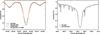 |
Fig. 1 Comparison of the IAG spectral atlas with the Kitt Peak FTS-atlas from Kurucz et al. (1984) and the HARPS atlas from Molaro et al. (2013). Left: three absorption lines around 524.85 nm. To allow comparison to the HARPS atlas, the IAG atlas was artificially broadened using a Gaussian profile and assuming an instrument resolution of R = 110 000. Right: comparison in the wavelength range of Hα. The sharp lines are telluric absorption and mismatch because of different observing conditions. The HARPS atlas does not cover this spectral region. |
5. Comparison of standard solar flux atlases
5.1. Overview
We consider three solar flux atlases for our comparison: two atlases taken with the FTS at Kitt Peak, and the HARPS LFC atlas. Before we discuss differences between the atlases, we summarize how the data were taken and the wavelength scales created.
5.1.1. Kitt Peak FTS atlas #1 −Kurucz et al. (1984)
Observations for this first Kitt Peak atlas were obtained with the McMath Solar Telescope at Kitt Peak National Observatory. In order to increase the S/N for each scan, data were taken in six different settings. Between 16 and 36 scans were averaged, two different beam-splitters and two different detectors were used (see Table 1 in Kurucz et al. 1984). Observations were carried out on six different days between November 23, 1980, and June 22, 1981. The wavenumber scale correction was determined from the telluric O2 line at 688.38335 nm in settings covering that line (#11 and #13). For the redmost setting (#15), the wavenumber scale was corrected by aligning terrestrial lines in common with the adjacent setting (#13). All other settings were corrected by aligning relatively clean solar lines in overlapping scans (Kurucz et al. 1984). A summary of the settings is given in Table 3. The authors estimate errors of the wavelength scale to be as large as 100 m s-1 in scan #1, errors in the other scans are estimated to be smaller. The scan lengths result in a broadening of 0.2 km s-1, the value of the middle time of observation was used for Doppler correction.
Settings and Doppler corrections used for the two Kitt Peak atlases.
5.1.2. Kitt Peak FTS atlas #2 −Wallace et al. (2011)
The second Kitt Peak FTS Atlas was pieced together from scans taken with the same instrument used for the first Kitt Peak FTS atlas. In addition, a version with telluric contamination removed by comparison with a spectrum taken at solar disk center is provided. Here we only refer to the uncorrected atlas. The specifications of the individual scans taken for this atlas are quite similar to the one from Kurucz et al. (1984), but a different set of scans was used for this atlas. A major difference is the way the Doppler correction was determined. For this second atlas, the Doppler correction was measured empirically; line positions of solar Fe i lines were measured and corrected to the frequencies reported in the catalogue by Nave et al. (1994). This implies that both gravitational redshift and the average velocity of the solar convective blueshift are removed from the atlas. Details of the individual scans and their Doppler corrections are summarized in Table 3. Electronic versions of the two Kitt Peak FTS atlases can be downloaded at ftp://vso.nso.edu/pub/
5.1.3. HARPS LFC atlas −Molaro et al. (2013)
A solar flux atlas from the HARPS spectrograph was obtained on Nov. 25, 2010, at La Silla observatory, Chile, from observations of the Moon. The spectra were taken at a resolution of R ~ 110 000, which means that in contrast to the FTS atlases, the solar lines are not fully resolved. The wavelength solution was created using external information from a spectrum taken with a LFC (Wilken et al. 2010). The accuracy of the LFC spectral lines is several factors higher than that of the intrinsic FTS solution and does not require any other correction. The spectra were used to discover variations in pixel size and distortions of the ThAr wavelength solution of the HARPS spectrograph. In November 2010, the LFC provided light useful for wavelength calibration in the range 476−530 nm and 534−585 nm; the two parts fall onto different detectors. The solar atlas is provided for this wavelengths range. The wavelength solution is corrected for barycentric motion.
5.2. Flux comparison
In the left panel of Fig. 1 we show a comparison between our new IAG atlas and the Kitt Peak FTS atlas #1 from Kurucz et al. (1984) and the HARPS LFC atlas from Molaro et al. (2013) in the region around an Fe i line. The right panel shows the comparison around Hα (the HARPS LFC atlas does not cover this region). The IAG atlas and the Kitt Peak atlas are in remarkable agreement in both regions. The sharp lines around Hα are telluric lines that reflect the very different observing conditions at the two sites. In the left panel, the lower spectral resolution of the HARPS atlas is evident. For comparison, we include an artificially broadened version of the IAG atlas assuming an additional Gaussian broadening according to an instrumental resolution of R = 110 000. The broadened spectrum is in very good agreement with the HARPS spectrum.
We conclude from this comparison that at the level of visual inspection, the three atlases compare to a very high degree. This shows that the three atlases do not differ significantly although they were taken with very different instruments. For example, one might have expected that scattered light could influence the HARPS spectrum more than the FTS spectra. Also, the level of the normalized continua are very similar although rather different standard procedures were applied to the unnormalized spectra. It is also apparent from Fig. 1 that the wavelength scales of the three spectra are very similar, which shows that barycentric corrections and conversion from air to vacuum wavelengths are consistently applied.
5.3. Wavelength scale comparison
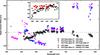 |
Fig. 2 Comparison of wavelength scales between different solar atlases − IAG atlas: this work; Kitt Peak atlas #1: Kurucz et al. (1984); Kitt Peak atlas #2: Wallace et al. (2011); HARPS LFC atlas: Molaro et al. (2013). Each data point shows the offset between two atlases calculated from a cross-correlation in a 2 nm range (see text). Comparisons between the IAG atlas and the two Kitt Peak atlases are shown in the main plot. Comparison between the HARPS atlas on the one hand and the IAG atlas and the Kitt Peak atlas from Kurucz et al. (1984) are shown in the inset. Only regions with little telluric contamination are shown. |
Precision spectroscopy currently investigates Doppler shifts at the level of m s-1, and future instrumentation is planned to be as precise as 10 cm s-1 (e.g., Pepe et al. 2010; Szentgyorgyi et al. 2014). As long as spectra are compared to others taken with the same instrument and consistent calibration methods, this precision can be achieved by securing stable calibration procedures. As soon as spectra are compared between different instruments, however, or if calibration procedures change, calibration must be tied to absolute standards for which the level of 1 m s-1 (3 × 10⁻⁹) is extremely difficult to reach. The faintness of astronomical targets is only one part of the problem; even with very bright sources in the laboratory, reaching an accuracy of ~10-9 is a very challenging task (see, e.g., Learner & Thorne 1988).
The way spectrographs are frequency- or wavelength-calibrated differs significantly between a grating spectrograph and an FTS. The three atlases used here are presumably calibrated to very high accuracy, but there are a number of effects that can deteriorate the final wavelength scale. In order to assess the wavelength calibrations of the four solar atlases, we compared the two Kitt-Peak FTS atlases and the HARPS LFC atlas against the IAG atlas, and checked consistency by comparing the two Kitt Peak atlases with each other and also checked the HARPS LFC atlas with Kitt Peak atlas #1. We calculated the RV offset between two atlases by cross-correlating them against each other in chunks of 2 nm. The cross-correlation function (CCF) was calculated in a range ±2 km s-1 around zero offset. The center of the CCF was determined by fitting a second-order polynomial to the three pixels around the maximum of the CCF, i.e., at the maximum pixel value and its two closest neighbors, and by determining the maximum of this polynomial. All atlases were corrected for barycentric correction, which means that spectral lines from the solar photosphere match between all atlases, but the positions of telluric lines differ. The cross-calibration provides a measure of fit quality between two spectra (similar to the χ2 value). We used this information to discard regions of strong telluric contamination, i.e., we reject regions in which the maximum value of the CCF indicated a mismatch between two spectra.
The results of our comparison are shown in Fig. 2 and summarized in Table 4. In Fig. 2 we can see substantial differences between individual data sets, and we can clearly distinguish the regions at which different Doppler corrections were applied to the FTS data. We discuss the RV offsets of the two Kitt Peak atlases, and the HARPS LFC atlas to the IAG atlas in the following.
5.3.1. Kitt Peak atlas #1
The absolute difference between the IAG atlas and the Kitt Peak FTS atlas #1 from Kurucz et al. (1984) is shown as open circles in Fig. 2. In the wavelength range 500−700 nm, the two wavelength scales are consistent within ±10 m s-1. A discontinuous step of approximately 10 m s-1 occurs at 576 nm. Blueward of 473 nm, a steep gradient can be seen that reaches down to an offset of ~−50 m s-1 at 430 nm. On the red side of the spectrum beyond 700 nm, a less steep gradient appears, the offset at 850 nm is approximately −20 m s-1. This analysis confirms the discussion of wavelength accuracy in Kurucz et al. (1984); the best agreement is reached around the range where the Kitt Peak atlas was anchored at the O2 line at 688 nm, and the difference between the wavelength scales increases with distance to the anchor point. Our new atlas does not extend to wavelengths shorter than 400 nm, but an extrapolation of the blueward trend between 400 and 500 nm is consistent with a maximum offset on the order of −100 m s-1 around 300 nm, as estimated in Kurucz et al. (1984). Not shown in Fig. 2 is the large offset at wavelengths beyond 1000 nm, the difference there is approximately + 300 m s-1 (see Table 4).
Differential comparison of wavelength scales between solar flux atlases.
5.3.2. Kitt Peak atlas #2
The comparison between the IAG atlas and the Kitt Peak FTS atlas #2 of Wallace et al. (2011) reveals interesting systematic effects (purple diamonds in Fig. 2). In the range 570−700 nm, the offset between the two atlases is approximately constant at a value of ≈+ 25 m s-1. Much larger deviations and systematic trends occur at other regions, for example a steep gradient between 440 nm and 570 nm, a large discontinuity (100 m s-1) at 570 nm, and offsets on the order of 200 m s-1 redward of 700 nm. We also provide offsets calculated between the two Kitt Peak atlases (purple plus symbols in Fig. 2). The differences between them are as large as 600 m s-1 at 300 nm (not shown in Fig. 2) and 200 m s-1 between 700 and 900 nm. The comparison clearly shows the consequences of using the solar lines as wavelength standards as is done in the atlas from Wallace et al. (2011). The values used for correcting a given wavelength range are essentially averages over all lines in each range, i.e., the correction depends on the distribution of the spectral lines, their formation depths, and the convective motion occurring at these depths. Since the distribution of line parameters over wavelengths is not smooth, several large jumps occur between the individual scan regions.
5.3.3. HARPS LFC atlas
From a comparison between the different FTS atlases, we can learn how their wavelength scales differ as a function of wavelength. It is not possible, however, to determine an accurate zero-point of the comparison at a level better than ±10 m s-1 because the FTS atlases used above (the IAG atlas and the Kitt Peak atlas #1) are anchored at telluric lines. A data set that is supposed to overcome this limitation is the LFC calibrated solar atlas from HARPS. The results of the comparison between the HARPS LFC atlas and the IAG atlas, and between the HARPS LFC atlas and the Kitt Peak atlas #1 are shown in the inset in Fig. 2 with filled red circles and black crosses, respectively. The HARPS LFC atlas and the IAG atlas show a systematic offset of (−5 ± 5) m s-1 with no significant trend (see Table 4; the uncertainty is the standard deviation of the offsets among the sample of 2 nm wide chunks). This is well within the estimated limits of accuracy determined by the uncertainty of telluric line positions used for the FTS wavelength correction. The lack of a significant trend bolsters our assumption that the wavelength scale of the IAG VIS atlas is intrinsically consistent across its wavelength range and accurate within the uncertainty of telluric line determination.
The comparison between the Kitt Peak atlas #1 and the HARPS LFC atlas reveals the same trend as the comparison between the IAG atlas and the Kitt peak atlas #1: between 534 nm and 585 nm the two atlases are consistent within uncertainties, but the average offset between 476 nm and 530 nm grows larger with a mean value of −30 m s-1 and a steep gradient reaching to −60 m s-1 as shown in Fig. 2.
6. Convective blueshift
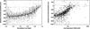 |
Fig. 3 Absolute convective blueshift of Fe i lines measured from the IAG atlas. Left: blueshift measurements for individual lines (gray points) as a function of line depth. The measurements are corrected for gravitational redshift of 636 m s-1. The median of the blueshift measurements is shown in bins of size 0.05; the error bars show the standard deviation for each bin. A third-order polynomial (Eq. (2)) is fit to the binned data. Right: blueshift measurements as a function of line equivalent width as measured by Allende Prieto & Garcia Lopez (1998). |
We make use of the IAG atlas to re-investigate the absolute convective blueshift of solar absorption lines and its dependence on line strength. We follow the strategy of Allende Prieto & Garcia Lopez (1998), who provided a comprehensive analysis of the blueshift of Fe i absorption lines as measured in the Kitt Peak atlas #1; the authors use lines between 400 nm and 750 nm. As shown above, the wavelength solution of the Kitt Peak atlas #1 shows some significant distortions at the wavelength range relevant for the blueshift study of Allende Prieto & Garcia Lopez (1998). We therefore re-determined the blueshift from our atlas.
For our analysis, we used the line list from Allende Prieto & Garcia Lopez (1998) and measured positions of the 1252 lines that are within the covered wavelength range (lines in the range 400−405 nm are not in our atlas). The center of each line was determined by fitting a second-order polynomial to the central ±4 km s-1 of each line; this corresponds to a range between 50 mÅ and 90 mÅ. Allende Prieto et al. used a range of 50 mÅ for all lines and fitted a fourth-order polynomial; we checked the consistency of our method to the results from Allende Prieto et al. by calculating the line centers in the Kitt Peak atlas #1. We calculated the difference between the measured line center and the laboratory line position as provided in the catalogue of Nave et al. (1994). In Fig. 3, we show the absolute convective blueshift of the 1252 Fe i lines as a function of line depth (left panel) and line equivalent width (right panel). We adopted the line equivalent widths from the compilation in Allende Prieto & Garcia Lopez (1998). All values of convective blueshift are corrected for the effect of gravitational redshift, i.e., an amount of 636 m s-1 was subtracted from our measured values to provide the absolute effect caused by the convective line shift. The individual values are provided in Table A.1 available at the CDS.
The individual line shifts in Fig. 3 show some scatter caused by measurement uncertainties and blends. We binned the individual data points in chunks of 0.05 units of normalized depth and show the median value together with the standard deviation in the left panel of Fig. 3; the values are also provided in Table 5 in steps of 0.1 depth units. A third-order polynomial fit to the binned data points is overplotted, the polynomial is ![Mathematical equation: \begin{equation} \label{eq:bspoly} \Delta v = -504.891 -43.7963 - 145.560 x^2 + 884.308 x^3 \ \left[\rm m\,s^{-1}\right] \end{equation}](/articles/aa/full_html/2016/03/aa27530-15/aa27530-15-eq42.png) (2)with x the relative line depth between 0.05 and 0.95.
(2)with x the relative line depth between 0.05 and 0.95.
Absolute convective blueshift as function of line depth.
The right panel of Fig. 3 shows the blueshift as a function of line equivalent width as in Fig. 2b of Allende Prieto & Garcia Lopez (1998). There are no significant differences between the overall appearances of the two plots. We disagree, however, with the conclusion from Allende Prieto et al. that lines located in the “plateau” with equivalent widths larger than ~100 mÅ are all blueshifted (see also Gray 2009). It appears that the strongest lines occur at the shortest wavelengths where the Kitt Peak solar atlas tends to overestimate the blueshift of the lines by several 10 m s-1. Our new determinations therefore show a systematically lower amount of blueshift in the strongest lines. Regardless of this systematic shift, we argue that the effect of a “plateau” is not real but rather the consequence of saturation. All spectral lines with equivalent widths larger than ~100 mÅ have line depths close to or above 90%. Stronger lines do not systematically probe higher regions in the stellar atmosphere but gain their larger equivalent width from growing line wings, hence higher formation heights of the wings and not the center.
7. Summary
We introduced the IAG solar flux atlas from 405 nm up to 2300 nm. The atlas was taken with an FTS in only two settings, one below approximately 1000 nm and a second one above this value. The fidelity of our atlas is similar to the Kitt Peak FTS atlases and we showed that the line depths are consistent between our atlas and the Kitt Peak atlases and also the atlas taken with HARPS. We summarized the instrumental characteristics used for the different atlases and argued that using only one setting for our entire VIS coverage (405−1065 nm) delivers a wavelength scale that is superior to the one in the Kitt Peak atlases where scans covering different wavelength ranges were stitched together. Our comparison revealed large systematic offsets between the two Kitt Peak atlases and also between the IAG atlas and the Kitt Peak atlases. This comes as no surprise because very different strategies for wavelength correction were used in the Kitt Peak atlases. For our NIR setting (1000−2300 nm), we did not perform a similar analysis in this paper.
Comparison of our wavelength scale to the one of the solar flux atlas taken with the HARPS spectrograph and calibrated using an LFC shows that the two scales are consistent within an uncertainty of only a few m s-1 as expected from the uncertainty in telluric line positions used for calibration in the IAG atlas. We conclude that the wavelength scale of the IAG atlas is precise and accurate to a level of ±10 m s-1. The atlas from Kurucz et al. (1984) is accurate to a level of 10 m s-1 in the limited wavelength range 530−570 nm, but the wavelength accuracy deteriorates to uncertainties as large as 60 m s-1 at 400 nm and probably more at shorter wavelengths as was written in the original publication. The wavelength scale of the atlas published in Wallace et al. (2011) is corrected for differences between solar lines and laboratory line measurements and therefore carries only limited information about absolute line positions. Systematic differences between this atlas and the others exceed values of 100 m s-1 at certain wavelengths.
We re-investigated convective blueshift in solar absorption lines as a function of line depth and equivalent width. We found that the systematic blueshift between 400 nm and 500 nm in the atlas from Kurucz et al. (1984) can lead to an underestimate of the blueshift in the strongest solar Fe i lines that can be found in that wavelength range. We found a steady decrease in the blueshift from approximately −550 m s-1 to around zero shift from very shallow (10% absorption) to very deep (90%) lines, respectively. We argued that there is no plateau at very large equivalent widths because lines with equivalent widths exceeding ~100 mÅ do not actually probe higher regions of the solar atmosphere.
Our new IAG atlas is a first attempt to provide high-accuracy and high-fidelity benchmark spectra useful for sub-m s-1 work, e.g., understanding the influence of convection on solar and stellar RV measurements. For the future, we aim to provide similar data for spatially resolved regions on the solar disk, and we are including an LFC in our facilities to provide an accurate wavelength calibration that overcomes the uncertainties of telluric line positions.
Salit el al. showed linearity to an accuracy of 6 × 10-9 = 2 m s-1 in their FTS in the wavelength range 320−670 nm. We believe that the linearity of our wavelength scale is not significantly different.
Acknowledgments
We thank the referee, X. Dumusque, for a very helpful report, H.-G. Ludwig for helpful discussions, and the team at IAG for their support with the observations. Part of this work was supported by the DFG funded SFB 963 Astrophysical Flow Instabilities and Turbulence and by the ERC Starting Grant Wavelength Standards, Grant Agreement Number 279347. A.R. acknowledges research funding from DFG grant RE 1664/9-1. The FTS was funded by the DFG and the State of Lower Saxony through the Großgeräteprogramm Fourier Transform Spectrograph.
References
- Allende Prieto, C., & Garcia Lopez, R. J. 1998, A&AS, 129, 41 [NASA ADS] [CrossRef] [EDP Sciences] [Google Scholar]
- Balthasar, H., Thiele, U., & Woehl, H. 1982, A&A, 114, 357 [NASA ADS] [Google Scholar]
- Davis, S. P., Abrams, M. C., & Brault, J. W. 2001, Fourier transform spectrometry (San Diego, CA: Academic Press) [Google Scholar]
- Dravins, D. 1982, ARA&A, 20, 61 [NASA ADS] [CrossRef] [Google Scholar]
- Dravins, D. 2008, A&A, 492, 199 [NASA ADS] [CrossRef] [EDP Sciences] [Google Scholar]
- Dravins, D., Lindegren, L., & Nordlund, A. 1981, A&A, 96, 345 [NASA ADS] [Google Scholar]
- Dumusque, X., Boisse, I., & Santos, N. C. 2014, ApJ, 796, 132 [NASA ADS] [CrossRef] [Google Scholar]
- Figueira, P., Pepe, F., Melo, C. H. F., et al. 2010, A&A, 511, A55 [NASA ADS] [CrossRef] [EDP Sciences] [Google Scholar]
- Gray, D. F. 2009, ApJ, 697, 1032 [NASA ADS] [CrossRef] [Google Scholar]
- Griffiths, P. R., & de Haseth, J. A. 2007, Fourier Transform Infrared Spectrometry, Second Edition (John Wiley) [Google Scholar]
- Kurucz, R. L., Furenlid, I., Brault, J., & Testerman, L. 1984, Solar flux atlas from 296 to 1300 nm [Google Scholar]
- Learner, R. C. M., & Thorne, A. P. 1988, J. Opt. Soc. Am. B, 5, 2045 [NASA ADS] [CrossRef] [Google Scholar]
- Meunier, N., & Lagrange, A.-M. 2013, A&A, 551, A101 [NASA ADS] [CrossRef] [EDP Sciences] [Google Scholar]
- Molaro, P., Esposito, M., Monai, S., et al. 2013, A&A, 560, A61 [NASA ADS] [CrossRef] [EDP Sciences] [Google Scholar]
- Nave, G., Johansson, S., Learner, R. C. M., Thorne, A. P., & Brault, J. W. 1994, ApJS, 94, 221 [NASA ADS] [CrossRef] [Google Scholar]
- Pepe, F. A., Cristiani, S., Rebolo Lopez, R., et al. 2010, in SPIE Conf. Ser., 7735, 77350F [Google Scholar]
- Saar, S. H., & Donahue, R. A. 1997, ApJ, 485, 319 [NASA ADS] [CrossRef] [Google Scholar]
- Salit, M. L., Sansonetti, C. J., Veza, D., & Travis, J. C. 2004, J. Opt. Soc. Am. B Opt. Phys., 21, 1543 [NASA ADS] [CrossRef] [Google Scholar]
- SILSO World Data Center 2014, International Sunspot Number Monthly Bulletin and online catalogue [Google Scholar]
- Szentgyorgyi, A., Barnes, S., Bean, J., et al. 2014, in SPIE Conf. Ser., 9147, 26 [Google Scholar]
- Wallace, L., Hinkle, K. H., Livingston, W. C., & Davis, S. P. 2011, ApJS, 195, 6 [NASA ADS] [CrossRef] [Google Scholar]
- Wilken, T., Lovis, C., Manescau, A., et al. 2010, in SPIE Conf. Ser., 7735, 77350T [Google Scholar]
All Tables
All Figures
|
Fig. 1 Comparison of the IAG spectral atlas with the Kitt Peak FTS-atlas from Kurucz et al. (1984) and the HARPS atlas from Molaro et al. (2013). Left: three absorption lines around 524.85 nm. To allow comparison to the HARPS atlas, the IAG atlas was artificially broadened using a Gaussian profile and assuming an instrument resolution of R = 110 000. Right: comparison in the wavelength range of Hα. The sharp lines are telluric absorption and mismatch because of different observing conditions. The HARPS atlas does not cover this spectral region. |
| In the text | |
|
Fig. 2 Comparison of wavelength scales between different solar atlases − IAG atlas: this work; Kitt Peak atlas #1: Kurucz et al. (1984); Kitt Peak atlas #2: Wallace et al. (2011); HARPS LFC atlas: Molaro et al. (2013). Each data point shows the offset between two atlases calculated from a cross-correlation in a 2 nm range (see text). Comparisons between the IAG atlas and the two Kitt Peak atlases are shown in the main plot. Comparison between the HARPS atlas on the one hand and the IAG atlas and the Kitt Peak atlas from Kurucz et al. (1984) are shown in the inset. Only regions with little telluric contamination are shown. |
| In the text | |
|
Fig. 3 Absolute convective blueshift of Fe i lines measured from the IAG atlas. Left: blueshift measurements for individual lines (gray points) as a function of line depth. The measurements are corrected for gravitational redshift of 636 m s-1. The median of the blueshift measurements is shown in bins of size 0.05; the error bars show the standard deviation for each bin. A third-order polynomial (Eq. (2)) is fit to the binned data. Right: blueshift measurements as a function of line equivalent width as measured by Allende Prieto & Garcia Lopez (1998). |
| In the text | |
Current usage metrics show cumulative count of Article Views (full-text article views including HTML views, PDF and ePub downloads, according to the available data) and Abstracts Views on Vision4Press platform.
Data correspond to usage on the plateform after 2015. The current usage metrics is available 48-96 hours after online publication and is updated daily on week days.
Initial download of the metrics may take a while.