| Issue |
A&A
Volume 587, March 2016
|
|
|---|---|---|
| Article Number | A28 | |
| Number of page(s) | 7 | |
| Section | Stellar structure and evolution | |
| DOI | https://doi.org/10.1051/0004-6361/201527320 | |
| Published online | 15 February 2016 | |
Zeeman-Doppler imaging of active young solar-type stars⋆
1
Department of Physics, PO Box 64 University of Helsinki
00084
Helsinki
Finland
e-mail:
This email address is being protected from spambots. You need JavaScript enabled to view it.
2
Department of Physics and Astronomy, Uppsala
University, Box
516, 751 20
Uppsala,
Sweden
3
ReSoLVE Centre of Excellence, Aalto University, Department of
Computer Science, PO Box
15400, 00076
Aalto,
Finland
Received: 7 September 2015
Accepted: 22 December 2015
Abstract
Context. By studying young magnetically active late-type stars, i.e. analogues to the young Sun, we can draw conclusions on the evolution of the solar dynamo.
Aims. We determine the topology of the surface magnetic field and study the relation between the magnetic field and cool photospheric spots in three young late-type stars.
Methods. High-resolution spectropolarimetry of the targets was obtained with the HARPSpol instrument mounted at the ESO 3.6 m telescope. The signal-to-noise ratios of the Stokes IV measurements were boosted by combining the signal from a large number of spectroscopic absorption lines through the least squares deconvolution technique. Surface brightness and magnetic field maps were calculated using the Zeeman-Doppler imaging technique.
Results. All three targets show clear signs of magnetic fields and cool spots. Only one of the targets, V1358 Ori, shows evidence of the dominance of non-axisymmetric modes. In two of the targets, the poloidal field is significantly stronger than the toroidal one, indicative of an α2-type dynamo, in which convective turbulence effects dominate over the weak differential rotation. In two of the cases there is a slight anti-correlation between the cool spots and the strength of the radial magnetic field. However, even in these cases the correlation is much weaker than in the case of sunspots.
Conclusions. The weak correlation between the measured radial magnetic field and cool spots may indicate a more complex magnetic field structure in the spots or spot groups involving mixed magnetic polarities. Comparison with a previously published magnetic field map shows that on one of the stars, HD 29615, the underlying magnetic field changed its polarity between 2009 and 2013.
Key words: polarization / stars: activity / stars: imaging / starspots
Based on observations made with the HARPSpol instrument on the ESO 3.6 m telescope at La Silla (Chile), under the program ID 091.D-0836.
© ESO, 2016
1. Introduction
Magnetic fields play a key role in the evolution of solar-type stars. They determine the angular momentum loss, shape stellar wind, produce high-energy electromagnetic and particle radiation, and influence the energy balance of planetary atmospheres.
The general notion as postulated by Parker (1955) is that the solar magnetic field is generated by an αΩ-dynamo: the toroidal field is generated by the winding up and simultaneous amplification of the poloidal field by differential rotation (Ω effect). The dynamo loop is closed by the collective inductive and diffusive effects arising from rotationally influenced convective turbulence, which generate small-scale poloidal fields from the underlying toroidal field (α effect), and the enhanced turbulent diffusion causing efficient reconnection to build up a large-scale poloidal field (β effect). In rapidly rotating late-type stars, the Ω effect is suppressed and therefore other types of dynamos, namely α2Ω or α2, are probably present (see e.g. Ossendrijver 2003, and references therein). In this case, the magnetic field is almost solely sustained by the α effect generating both poloidal and toroidal fields. Typical αΩ solutions show dominance of the toroidal component, whereas the other types of solutions have more equal energies in both of the components of the surface field.
Young late-type stars are generally rapidly rotating owing to the large angular momentum remaining from the contraction phase during early stellar evolution. Because of magnetic braking the rotation slows down. This means that as a solar-type star evolves, its dynamo will move from the α2 or α2Ω-regime to an αΩ-dynamo. In order to properly understand the mechanism and evolution of the dynamos of solar-type stars it is essential to study stars of different ages.
To investigate young solar-type stars, we initiated a programme called “Active Suns” for the observation of a small sample of young solar analogues with the HARPSpol instrument mounted at the ESO 3.6 m telescope at La Silla (Chile). The three stars in this study, AH Lep, HD 29615 and V1358 Ori, are located at the more rapidly rotating and thus more magnetically active end of our small sample.
Our primary aims were to determine the topology of the surface magnetic field and to study the relation between magnetic fields and cool spots. For this purpose we applied the Zeeman-Doppler imaging (ZDI) technique using Stokes IV spectropolarimetry with a code developed by O. Kochukhov (Kochukhov et al. 2014).
2. Observations
Stokes IV spectropolarimetry was collected with the HARPSpol spectropolarimeter mounted at the ESO 3.6 m telescope at La Silla, Chile through the programme “Active Suns” (091.D-0836). HARPS itself is a fibre-fed, cross-dispersed échelle spectrograph described in greater detail by Mayor et al. (2003). The polarisation unit HARPSpol is installed at the Cassegrain focus (Piskunov et al. 2011). The normal procedure for obtaining a Stokes V profile is to use four sub-exposures with a rotation of 90° of the quarter-wave plate between each sub-exposure. This procedure allows the calculation of a “null spectrum”, which should only contain noise and is thus a way to check that there is no spurious signal contaminating the Stokes V profile.
The observations were reduced using the REDUCE package (Piskunov & Valenti 2002). The standard reduction procedure included bias subtraction, flat fielding by a normalised flat field spectrum, subtraction of scattered light, and an optimal extraction of the spectral orders. The blaze function of the échelle spectrometer was removed to first order by dividing the observed stellar spectra by a smoothed spectrum of the flat field lamp. The continuum normalisation was performed by fitting a second-order polynomial to the blaze-corrected spectra. A consistent continuum normalisation procedure was applied to the spectra extracted from all sub-exposures. The wavelength solution for each spectrum was accomplished by fitting a two-dimensional polynomial, for approximately 1000 extracted thorium lines observed from the internal lamp assembly.
The spectral resolution of the reduced observations was R ≈ 105 000. The rotation phase coverage (fφ) for each star was estimated assuming that each observation covers a phase range of [ φrot − 0.05,φrot + 0.05], as suggested by Kochukhov et al. (2013). The observations are summarised in Table 1 and listed in Table 2.
Since the aim of the Stokes V observations was to map the surface magnetic field, the high demand for the signal-to-noise ratio (S/N) was far beyond what could be reached for individual photospheric absorption lines within reasonable exposure times. In order to boost the S/N a large number of photospheric absorption lines in the wavelength range 3800−6900 Å were combined with least squares deconvolution (LSD; Donati et al. 1997; Kochukhov et al. 2010). The line mask for the LSD procedure was obtained from the VALD data base (Piskunov et al. 1995; Kupka et al. 1999). Regions dominated by strong lines were avoided, since the profile of strong lines deviates from the average line profile. More details on the LSD procedure can be found in the paper by Kochukhov et al. (2014). The final S/N of the LSD profiles was 5000−12 000 in the Stokes V spectra. The LSD profiles were calculated on a radial velocity grid with a 1.6 km s-1 step size. The number of spectral lines used in the LSD mask for each star is listed in Table 1. The same masks were used for both the Stokes I and V.
From the LSD Stokes V spectra we calculated the false alarm probabilities (FAP) for each observations using the reduced χ2 statistics (see e.g. Donati et al. 1992; Rosén et al. 2013) and the radial velocity range [−vsini − 7.0 km s-1, vsini + 7.0 km s-1]. Each point of the Stokes V profile had its own error estimate σi corresponding to the S/N. This σi was used for the calculation of the FAP values. The same procedure was also followed for the null spectra, which naturally reached the same S/N level as the Stokes V. The minimum FAP values for the Stokes V profiles of the targets are listed in Table 1 and all FAP values for both the Stokes V and the null profiles are listed in Table 2. Using a FAP limit of 10-5 we concluded that all three targets showed definite detection of a magnetic field. We also evaluated the mean longitudinal magnetic field ⟨ BZ ⟩ from the first moment of the Stokes V profile as described by Kochukhov et al. (2010) for both the Stokes V observations and the null spectra using the same radial velocity range as for the FAP. These measurements are listed in Table 2. The ⟨ BZ ⟩ for each stellar observation as a function of the rotation phase is plotted in Fig. 1. The errors on ⟨ BZ ⟩ were estimated by propagating the errors on the observations. The null spectra are plotted in Fig. 2.
Summary of observations with HARPSpol at the ESO 3.6 m telescope.
Observations with HARPSpol at the ESO 3.6 m telescope.
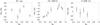 |
Fig. 1 Mean longitudinal magnetic field as a function of rotational phase. From left to right: AH Lep, HD 29615, and V1358 Ori. |
3. Zeeman-Doppler imaging
The Stokes V profiles were modelled assuming the weak field approximation, i.e. that the local Stokes V profile is proportional to the effective Landé g-factor. The Landé factor was determined as suggested by Kochukhov et al. (2010) and the values are listed in Table 3.
The Stokes I profiles were modelled using a temperature independent analytical Voigt function. For neutral photospheric metal lines, the absorption is usually larger in a cool spot than in the unspotted photosphere for solar-type stars. This effect is, however, of secondary importance because the reduced continuum level in the spot will dominate. Thus, for all photospheric absorption lines, the spot will be observable as an “emission” bump moving across the line as the star rotates. The amplitude of the bump will, of course, depend on the changing equivalent width of the absorption line. Therefore, the approximation of constant line profile should only lead to a slight error in the retrieved brightness of the spots and the overall equivalent width of the line (as this usually becomes slightly stronger when large cool spots reduce the observed mean Teff).
Similar approximations to those used in this study are commonly used in ZDI for the Stokes IV when applying the LSD technique (see e.g. Petit et al. 2004). An alternative would be to treat the LSD profiles as a single line with average parameters or derive the local LSD profile from the full spectrum synthesis. The former still involves approximations and so the advantages are limited. The latter is feasible for early-type stars (see e.g. Kochukhov et al. 2014), but much more demanding for late-type stars when imaging both the surface magnetic field and temperature (or brightness). Furthermore, none of the stars in this study showed any strong bumps in the Stokes I, reducing the error of the approximation.
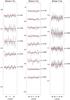 |
Fig. 2 Stokes V null profiles. The error bars are drawn as vertical lines through the data points and the 0-level is shown with a red line. From left to right: AH Lep, HD 29615, and V1358 Ori. |
We used the inversLSD code developed by O. Kochukhov. The stellar surface was divided into 1876 spatial elements. The magnetic inversion was based on a spherical harmonics expansion, as described by e.g. Kochukhov et al. (2014) and Rosén et al. (2015). One of the advantages with this approach is that one can easily determine the amount of energy contained in the toroidal and poloidal components of the magnetic field, as well as the different ℓ-modes.
To set the highest allowed ℓ-mode, different values of ℓmax from 3 to 10 were tested. In the solutions with ℓmax> 5, smaller scale structures appeared even though the fits to the Stokes V observations were not found to be significantly improved. This tendency was independent of the vsini-value, which regulates the expected surface resolution for temperature Doppler imaging. This implies that Stokes V alone is not sensitive to small-scale features of higher order ℓ-modes. In fact, Rosén et al. (2015) have shown that recovering such details would also require using linear Stokes QU polarisation measurements. The maximum was therefore set to ℓmax = 5 for all stars regardless of their rotational velocities.
The magnetic field inversion was regularised with a harmonic penalty function, while we used Tikhonov regularisation for the brightness inversion (see e.g. Rosén et al. 2015). In addition to the Tikhonov regularisation we also introduced an extra penalty function to restrain the surface brightness within values of [ 0.5,1.5], with 1.0 corresponding to the unspotted surface:
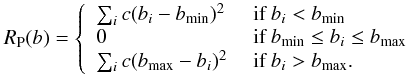 Here bmin and bmax are the allowed minimum and maximum values for the brightness bi, and c is a constant. This extra restriction was necessary because using the approximation of a constant local Stokes I profile made the brightness inversion insensitive to the mean brightness.
The inverse solution was obtained using the Levenberg-Marquardt minimisation. Here the first and second derivatives of the extra penalty function RP were calculated analytically. The magnetic energy contained in the axisymmetric and non-axisymmetric harmonic components was calculated using the same definition as in Fares et al. (2009): modes with m<ℓ/ 2 were defined as axisymmetric and those with m ≥ ℓ/ 2 considered non-axisymmetric.
4. Observed stars and their adopted stellar parameters
The three stars in this study are nearby young solar-type and they are effectively single stars, in the sense that they lack any companions close enough for detectable interaction. AH Lep and V1358 Ori are believed to belong to the local association, implying ages of 20−150 Myr (see e.g. Montes et al. 2001), while HD 29615 has been proposed as a member of the Tucana/Horologium association indicating an age of ~30 Myr (see e.g. Zuckerman et al. 2011). They are, however, slightly hotter than the young Sun. For one of the stars, V1358 Ori, there are no previously published ZDI studies. Previous ZDI maps of AH Lep and HD29615 were presented by Carter et al. (2015) and Waite et al. (2015).
Summary of the adopted parameters.
4.1. AH Lep
AH Lep (HD 36869, TYC 5916-792-1) is classified as a G3V star (Montes et al. 2001) with a TYCHO catalogue parallax of 28.6 mas (Wichmann et al. 2003), i.e. a distance of r ≈ 35pc. Zuckerman et al. (2011) reported an effective temperature of Teff ≈ 5800 K and a radius of R ≈ 1.21 R⊙. Cutispoto et al. (1999) calculated a photometric rotation period of  . Messina et al. (2003) reported a maximum photometric amplitude of 0.09 in the V magnitude and an X-ray flux of lg(LX/Lbol) = −3.480. Our best fit to the Stokes I profile was achieved with a rotation velocity of vsini = 26.3 km s-1, i.e. close to the value of 27.3 km s-1 measured by López-Santiago et al. (2010). Combining the previously measured radius, rotation period and our rotation velocity estimate we retrieved an inclination of the rotation axis of i ≈ 36°. To calculate the rotation phases (φrot in Table 2) of the spectropolarimetric observations, we used the ephemeris

4.2. HD 29615
HD 29615 (HIP 21632, TYC 6467-702-1) has a Simbad spectral classification of G3V (Torres et al. 2006). Its Hipparcos parallax is 17.8 mas (van Leeuwen 2007) giving a distance of r ≈ 56 pc. According to McDonald et al. (2012) its effective temperature is Teff ≈ 5866 K. Vidotto et al. (2014) reported a radius of R ≈ 0.96 R⊙ and a rotation period of  . Messina et al. (2010) reported a photometric amplitude of AV = 0.08. We estimated the rotation velocity to be vsini ≈ 18.5 km s-1 giving an inclination angle of i ≈ 62°. Our observations were phased with the ephemeris
 Recently Waite et al. (2015) published a ZDI study of HD 29615, where they also estimated the differential rotation of the star. Expressed as the differential rotation coefficient k = ΔΩ/Ω, they searched for the value of k that gave the best fit to the observations and reported k ≈ 0.18 from the magnetic field structures and k ≈ 0.026 from the temperature spot structures. In principle, a discrepancy between these values could be caused by different anchor depths. However, such a huge difference seems unlikely. Furthermore, theoretical considerations (see e.g. Krause & Rädler 1980) and numerical simulations (e.g. Kitchatinov & Olemskoy 2011; Cole et al. 2014) indicate that the magnetic fields of rapidly rotating solar-type stars are only weakly influenced by differential rotation, and they are therefore expected to have very small values of k. Thus, and especially since we simultaneously retrieve both the magnetic field and surface brightness, we did not apply any surface differential rotation in this study.
 |
Fig. 3 ZDI maps of AH Lep in equirectangular projection. The dashed vertical lines mark the observed rotation phases and the pointed horizontal line the limit of visibility due to the stellar inclination. |
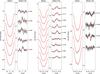 |
Fig. 6 The Stokes IV observations (plus signs/crosses) and profiles (solid line in red) calculated from the ZDI solutions. The error bars for the Stokes V observations are drawn as vertical lines through the data points. From left to right: AH Lep, HD 29615, and V1358 Ori. |
4.3. V1358 Ori
V1358 Ori (HD 43989, HIP 30030, TYC 4788-1272-1) was classified as a F9V-type star by Montes et al. (2001). van Leeuwen (2007) reported a Hipparcos parallax of 20.31 mas, placing it at a distance of r ≈ 49 pc. McDonald et al. (2012) reported an effective temperature of Teff ≈ 6032 K, while the estimate of Vican & Schneider (2014) was Teff ≈ 6100 K. Furthermore, Vican & Schneider (2014) reported a radius of R ≈ 1.05 R⊙, while Zuckerman et al. (2011) presented the value R ≈ 1.08 R⊙. We adopted the value 1.1 R⊙. From photometric observations Cutispoto et al. (2003) calculated a rotation period of  and estimated the photometric amplitude to be AV = 0.08. Furthermore, they reported an X-ray flux of lg(LX/Lbol) = −3.629. We estimated the rotation velocity to be vsini ≈ 41.3 km s-1, giving an inclination of i ≈ 59°. To phase our observations, we used the ephemeris

5. Results
The resulting ZDI-maps are presented in Figs. 3–5 and their corresponding Stokes I and V profiles in Fig. 6. The strongest magnetic field is detected on HD 29615 and the weakest field on V1358 Ori (Table 4). HD 29615 shows an almost axisymmetric structure with both the magnetic field and cool spots concentrated at high latitudes around the pole. In V1358 Ori the axisymmetric component of the field is stronger than the non-axisymmetric. AH Lep, on the other hand, has clearly non-axisymmetric geometries of both the magnetic fields and cool spots. It should be noted, however, that the ZDI maps of AH Lep and V1358 Ori are based on poor phase coverages.
The poloidal component dominates the surface fields of AH Lep and HD 29615, while the toroidal component is stronger for V1358 Ori. In terms of complexity, the ℓ = 1 mode dominates the fields of HD 29615 and V1358 Ori, while ℓ = 2 is strongest for AH Lep (containing 31.2% of the magnetic energy). The information on the magnetic field of each star is summarised in Table 4. This table lists the maximum detected surface field (Bmax) and the percentage of magnetic energy contained in the different components of the field (toroidal/poloidal, axisymmetric/non-axisymmetric and ℓ = 1 mode).
We also calculated the linear correlation between the magnetic field maps and surface brightness maps. The correlation between the radial magnetic field (| Br |) and surface brightness (b) is especially interesting. In the solar case cool spots are, of course, concentrated in regions were strong magnetic fields penetrate the surface. This implies a strong negative correlation r( | Br | ,b). We could only find a weak correlation for the three stars, and in the case of V1358 Ori the correlation coefficient is positive, i.e. of an opposite sign than expected (Table 4). Again, poor phase coverage may play a role.
Summary of magnetic field detection.
6. Conclusions
We see considerable differences in the topology of the surface magnetic fields of the three stars in this study. Since the stars themselves are evolutionarily and structurally close, it is likely that these differences reflect temporal changes rather than different dynamo mechanisms.
We only have three snapshots, which means that far reaching conclusions cannot be drawn from our study. However, the poloidal and toroidal components are of same order of magnitude in all three targets, which is a strong indication of a dynamo of α2 or α2Ω type (cf. Käpylä et al. 2013, where dynamos of different types are compared in direct numerical simulations). On the other hand, the clear dominance of the axisymmetric mode in two of the three targets is somewhat unexpected from mean-field dynamo theory (e.g. Krause & Rädler 1980). Again, this could be due to the non-stationarity over time, i.e. caused by the targets being at different phases of the oscillatory dynamo cycle. This conclusions is not at odds with the proposed type of the dynamo, as even for α2 dynamos, oscillatory solutions can be expected (see Käpylä et al. 2013, and references therein).
The previous ZDI study of HD 29615 was based on observations collected in November–December 2009 (Waite et al. 2015). These ZDI maps look quite similar to our maps. In both cases the magnetic field is dominated by a strong radial field centred near the rotational pole that covers the whole polar region. Interestingly, the polarity in the 2009 map is opposite to that in our map. Thus, the star has undergone a polarity reversal between December 2009 and September 2013. The brightness maps similarly show a high latitude spot structure clearly offset from the strongest radial field.
When studying the correlation between the magnetic field and temperature spots, one must remember that the detectability of the field is weighted by the surface brightness. If this were the reason for the dark spots not coinciding with strong magnetic fields, one would expect the detected magnetic field strength to be correlated with the surface brightness. Only for the case of V1358 Ori do we observe such a weak trend, and even then this is most likely biased by the poor phase coverage. On the other hand, Rosén & Kochukhov (2012) showed that the ZDI method is capable of reproducing both the magnetic field and cool spot structures in cases where they coincide. In the case of our maps of AH Lep and especially of V1358 Ori, the poor phase coverage makes the comparison of magnetic and brightness maps uncertain. However, while some exceptions exist (see e.g. Carroll et al. 2012), in most cases where surface magnetic field and temperature, brightness, or spot occupancy maps have been retrieved from the same spectropolarimetric data, there seems to be a discrepancy between the concentration of cool spots and magnetic fields (see e.g. Jeffers et al. 2011; Kochukhov et al. 2013; Waite et al. 2015).
A possible explanation for the lack of correlation between cool spots and a detected magnetic field could be that the large spots seen in Doppler images are actually spot groups with mixed polarity. In this case the surface resolution of the ZDI is not able to distinguish the detailed magnetic field configuration. The images would thus only display a larger scale field. If this were the case, one would expect the lifetimes of the spot structures to be very short as many magnetic flux tubes of opposite polarities packed tightly together would reconnect and decay rapidly. This would most likely manifest itself through line profile variations, and the time scale of changes would be helpful in providing indirect evidence of the topology of the unresolved structures. Unfortunately, the limited time span of our observations does not allow for such an analysis. The situation is further complicated because temperature spots can be generated without magnetic fields through vortex instability, as demonstrated by e.g. Käpylä et al. (2011) and Mantere et al. (2011).
Rosén et al. (2015) compared ZDI results retrieved using just Stokes IV with the full set of Stokes IVQU components for the RS CVn star II Peg. They found few differences in the temperature maps, but significant differences in the magnetic field solutions. The retrieval of the meridional field component especially benefited from using the linear Stokes QU components. Furthermore, using just Stokes IV resulted in an underestimation of the total magnetic energy. Therefore, we can expect that the real surface magnetic fields of our targets are stronger and much more complex than indicated by this study.
Despite these shortcomings, the results of this study can be used to retrieve information on possible stellar magnetic cycles. Here it is especially interesting to follow the evolution of the poloidal and toroidal components and the complexity of the field, and to detect polarity reversals of the large-scale field. Such reversals have been seen in many stars and with this study we can add HD 29615 to this group.
Acknowledgments
This research has made use of the SIMBAD database operated at CDS, Strasbourg, France. T.H. was partly supported by the “Active Suns” research project at the University of Helsinki. J.L. was supported by the Vilho, Yrjö, and Kalle Väisälä Foundation. OK is a Royal Swedish Academy of Sciences Research Fellow, supported by grants from the Knut and Alice Wallenberg Foundation and Swedish Research Council. M.J.K. acknowledges financial support from the Academy of Finland Centre of Excellence ReSoLVE (grant No. 272157). The authors thank the anonymous referee for useful comments that helped improve the manuscript.
References
- Carroll, T. A., Strassmeier, K. G., Rice, J. B., & Künstler, A. 2012, A&A, 548, A95 [NASA ADS] [CrossRef] [EDP Sciences] [Google Scholar]
- Carter, B. D., Marsden, S. C., & Waite, I. A. 2015, in 18th Cambridge Workshop on Cool Stars, Stellar Systems, and the Sun, eds. G. T. van Belle, & H. C. Harris, 18, 209 [Google Scholar]
- Cole, E., Käpylä, P. J., Mantere, M. J., & Brandenburg, A. 2014, ApJ, 780, L22 [NASA ADS] [CrossRef] [Google Scholar]
- Cutispoto, G., Pastori, L., Tagliaferri, G., Messina, S., & Pallavicini, R. 1999, A&AS, 138, 87 [NASA ADS] [CrossRef] [EDP Sciences] [Google Scholar]
- Cutispoto, G., Messina, S., & Rodonò, M. 2003, A&A, 400, 659 [NASA ADS] [CrossRef] [EDP Sciences] [Google Scholar]
- Donati, J.-F., Semel, M., & Rees, D. E. 1992, A&A, 265, 669 [NASA ADS] [Google Scholar]
- Donati, J.-F., Semel, M., Carter, B. D., Rees, D. E., & Collier Cameron, A. 1997, MNRAS, 291, 658 [NASA ADS] [CrossRef] [MathSciNet] [Google Scholar]
- Fares, R., Donati, J.-F., Moutou, C., et al. 2009, MNRAS, 398, 1383 [NASA ADS] [CrossRef] [MathSciNet] [Google Scholar]
- Jeffers, S. V., Donati, J.-F., Alecian, E., & Marsden, S. C. 2011, MNRAS, 411, 301 [NASA ADS] [CrossRef] [Google Scholar]
- Käpylä, P. J., Mantere, M. J., & Hackman, T. 2011, ApJ, 742, 34 [NASA ADS] [CrossRef] [Google Scholar]
- Käpylä, P. J., Mantere, M. J., & Brandenburg, A. 2013, Geophys. Astrophys. Fluid Dyn., 107, 244 [Google Scholar]
- Kitchatinov, L. L., & Olemskoy, S. V. 2011, MNRAS, 411, 1059 [NASA ADS] [CrossRef] [Google Scholar]
- Kochukhov, O., Makaganiuk, V., & Piskunov, N. 2010, A&A, 524, A5 [NASA ADS] [CrossRef] [EDP Sciences] [Google Scholar]
- Kochukhov, O., Mantere, M. J., Hackman, T., & Ilyin, I. 2013, A&A, 550, A84 [NASA ADS] [CrossRef] [EDP Sciences] [Google Scholar]
- Kochukhov, O., Lüftinger, T., Neiner, C., Alecian, E., & MiMeS Collaboration 2014, A&A, 565, A83 [NASA ADS] [CrossRef] [EDP Sciences] [Google Scholar]
- Krause, F., & Rädler, K.-H. 1980, Mean-field magnetohydrodynamics and dynamo theory (Oxford: Pergamon press) [Google Scholar]
- Kupka, F., Piskunov, N., Ryabchikova, T. A., Stempels, H. C., & Weiss, W. W. 1999, A&AS, 138, 119 [NASA ADS] [CrossRef] [EDP Sciences] [MathSciNet] [PubMed] [Google Scholar]
- López-Santiago, J., Montes, D., Gálvez-Ortiz, M. C., et al. 2010, A&A, 514, A97 [NASA ADS] [CrossRef] [EDP Sciences] [Google Scholar]
- Mantere, M. J., Käpylä, P. J., & Hackman, T. 2011, Astron. Nachr., 332, 876 [NASA ADS] [CrossRef] [Google Scholar]
- Mayor, M., Pepe, F., Queloz, D., et al. 2003, The Messenger, 114, 20 [NASA ADS] [Google Scholar]
- McDonald, I., Zijlstra, A. A., & Boyer, M. L. 2012, MNRAS, 427, 343 [NASA ADS] [CrossRef] [Google Scholar]
- Messina, S., Pizzolato, N., Guinan, E. F., & Rodonò, M. 2003, A&A, 410, 671 [NASA ADS] [CrossRef] [EDP Sciences] [Google Scholar]
- Messina, S., Desidera, S., Turatto, M., Lanzafame, A. C., & Guinan, E. F. 2010, A&A, 520, A15 [NASA ADS] [CrossRef] [EDP Sciences] [Google Scholar]
- Montes, D., López-Santiago, J., Gálvez, M. C., et al. 2001, MNRAS, 328, 45 [NASA ADS] [CrossRef] [MathSciNet] [Google Scholar]
- Ossendrijver, M. 2003, A&ARv, 11, 287 [Google Scholar]
- Parker, E. N. 1955, ApJ, 122, 293 [NASA ADS] [CrossRef] [Google Scholar]
- Petit, P., Donati, J.-F., Wade, G. A., et al. 2004, MNRAS, 348, 1175 [NASA ADS] [CrossRef] [Google Scholar]
- Piskunov, N. E., & Valenti, J. A. 2002, A&A, 385, 1095 [NASA ADS] [CrossRef] [EDP Sciences] [Google Scholar]
- Piskunov, N. E., Kupka, F., Ryabchikova, T. A., Weiss, W. W., & Jeffery, C. S. 1995, A&AS, 112, 525 [NASA ADS] [Google Scholar]
- Piskunov, N., Snik, F., Dolgopolov, A., et al. 2011, The Messenger, 143, 7 [NASA ADS] [Google Scholar]
- Rosén, L., & Kochukhov, O. 2012, A&A, 548, A8 [NASA ADS] [CrossRef] [EDP Sciences] [Google Scholar]
- Rosén, L., Kochukhov, O., & Wade, G. A. 2013, MNRAS, 436, L10 [NASA ADS] [CrossRef] [Google Scholar]
- Rosén, L., Kochukhov, O., & Wade, G. A. 2015, ApJ, 805, 169 [NASA ADS] [CrossRef] [Google Scholar]
- Torres, C. A. O., Quast, G. R., da Silva, L., et al. 2006, A&A, 460, 695 [NASA ADS] [CrossRef] [EDP Sciences] [Google Scholar]
- van Leeuwen, F. 2007, A&A, 474, 653 [NASA ADS] [CrossRef] [EDP Sciences] [Google Scholar]
- Vican, L., & Schneider, A. 2014, ApJ, 780, 154 [NASA ADS] [CrossRef] [Google Scholar]
- Vidotto, A. A., Gregory, S. G., Jardine, M., et al. 2014, MNRAS, 441, 2361 [NASA ADS] [CrossRef] [Google Scholar]
- Waite, I. A., Marsden, S. C., Carter, B. D., et al. 2015, MNRAS, 449, 8 [NASA ADS] [CrossRef] [Google Scholar]
- Wichmann, R., Schmitt, J. H. M. M., & Hubrig, S. 2003, A&A, 399, 983 [NASA ADS] [CrossRef] [EDP Sciences] [Google Scholar]
- Zuckerman, B., Rhee, J. H., Song, I., & Bessell, M. S. 2011, ApJ, 732, 61 [NASA ADS] [CrossRef] [Google Scholar]
All Tables
All Figures
|
Fig. 1 Mean longitudinal magnetic field as a function of rotational phase. From left to right: AH Lep, HD 29615, and V1358 Ori. |
| In the text | |
|
Fig. 2 Stokes V null profiles. The error bars are drawn as vertical lines through the data points and the 0-level is shown with a red line. From left to right: AH Lep, HD 29615, and V1358 Ori. |
| In the text | |
|
Fig. 3 ZDI maps of AH Lep in equirectangular projection. The dashed vertical lines mark the observed rotation phases and the pointed horizontal line the limit of visibility due to the stellar inclination. |
| In the text | |
 |
Fig. 4 Same as Fig. 3 for HD 29615. |
| In the text | |
 |
Fig. 5 Same as Fig. 3 for V1358 Ori. |
| In the text | |
|
Fig. 6 The Stokes IV observations (plus signs/crosses) and profiles (solid line in red) calculated from the ZDI solutions. The error bars for the Stokes V observations are drawn as vertical lines through the data points. From left to right: AH Lep, HD 29615, and V1358 Ori. |
| In the text | |
Current usage metrics show cumulative count of Article Views (full-text article views including HTML views, PDF and ePub downloads, according to the available data) and Abstracts Views on Vision4Press platform.
Data correspond to usage on the plateform after 2015. The current usage metrics is available 48-96 hours after online publication and is updated daily on week days.
Initial download of the metrics may take a while.