| Issue |
A&A
Volume 587, March 2016
|
|
|---|---|---|
| Article Number | A120 | |
| Number of page(s) | 8 | |
| Section | Interstellar and circumstellar matter | |
| DOI | https://doi.org/10.1051/0004-6361/201527148 | |
| Published online | 29 February 2016 | |
Accuracy requirements to test the applicability of the random cascade model to supersonic turbulence
École Normale Supérieure, Lyon, CRAL, UMR CNRS 5574, Université de
Lyon,
69342
Lyon,
France
e-mail:
doris.folini@ens-lyon.fr
Received: 9 August 2015
Accepted: 21 January 2016
A model, which is widely used for inertial rang statistics of supersonic turbulence in the context of molecular clouds and star formation, expresses (measurable) relative scaling exponents Zp of two-point velocity statistics as a function of two parameters, β and Δ. The model relates them to the dimension D of the most dissipative structures, D = 3 − Δ/(1 − β). While this description has proved most successful for incompressible turbulence (β = Δ = 2/3, and D = 1), its applicability in the highly compressible regime remains debated. For this regime, theoretical arguments suggest D = 2 and Δ = 2/3, or Δ = 1. Best estimates based on 3D periodic box simulations of supersonic isothermal turbulence yield Δ = 0.71 and D = 1.9, with uncertainty ranges of Δ ∈ [0.67,0.78] and D ∈ [2.04,1.60]. With these 5−10% uncertainty ranges just marginally including the theoretical values of Δ = 2/3 and D = 2, doubts remain whether the model indeed applies and, if it applies, for what values of β and Δ. We use a Monte Carlo approach to mimic actual simulation data and examine what factors are most relevant for the fit quality. We estimate that 0.1% (0.05%) accurate Zp, with p = 1,...,5, should allow for 2% (1%) accurate estimates of β and Δ in the highly compressible regime, but not in the mildly compressible regime. We argue that simulation-based Zp with such accuracy are within reach of today’s computer resources. If this kind of data does not allow for the expected high quality fit of β and Δ, then this may indicate the inapplicability of the model for the simulation data. In fact, other models than the one we examine here have been suggested.
Key words: shock waves / hydrodynamics / ISM: kinematics and dynamics / gamma-ray burst: general / binaries: close / turbulence
© ESO, 2016
1. Introduction
Supersonic turbulence is a key ingredient in various astrophysical contexts, from gamma ray bursts (Lazar et al. 2009; Narayan & Kumar 2009) or stellar accretion (Walder et al. 2008; Hobbs et al. 2011) to molecular clouds and star formation (Chabrier & Hennebelle 2011; Federrath & Klessen 2012; Padoan et al. 2012; Kritsuk et al. 2013). A key question is whether this turbulence, like incompressible turbulence, is characterized by universal statistics. Results from 3D periodic box simulations of driven, isothermal, supersonic turbulence (Kritsuk et al. 2007a; Schmidt et al. 2008; Pan et al. 2009) are indeed consistent with the highly compressible variant (Boldyrev 2002) of the hierarchical structure model that was put forward by She & Leveque (1994) for incompressible turbulence and that was further scrutinized by Dubrulle (1994) and She & Waymire (1995). This model is correspondingly popular in astrophysics. It is employed, for example, in the interpretation of molecular cloud observations (Gustafsson et al. 2006; Hily-Blant et al. 2008) or to derive a theoretical expression for the density distribution in supersonic turbulence (Boldyrev et al. 2002), which enters theories of the stellar initial mass function (Hennebelle & Chabrier 2008).
Nevertheless, some doubts remain whether the model really applies to simulation data of supersonic turbulence and, if so, with what parameter values. The best-fit model parameters that we are aware of (Pan et al. 2009) still come with a 5−10% uncertainty range that is only marginally compatible with theoretically predicted parameter values (see below). Here we argue that today’s computer resources should allow for 1−2% accurate parameter fits in the highly compressible regime, thereby likely settling the issue. Our claim is based on a Monte Carlo approach to mimic actual simulation data.
The hierarchical structure model predicts the ratios Zp of (observable) structure function scaling exponents ζp, p = 1,2,3,... etc., of a 3D velocity field u as 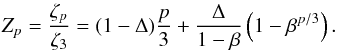 (1)Here, D = 3 − C is the dimension of the most intermittent structure, C = Δ/(1 − β) the associated co-dimension, β ∈ [0,1] measures the intermittency of the energy cascade, and Δ ∈ [0,1] measures the divergent scale dependence of the most intermittent structures. The ζp are defined in the inertial range by
  (2)where ⟨ ... ⟩ denotes the average over all positions x within the sample and over all directed distances r. The Zp should be well defined over a larger range because of extended self-similarity (Benzi et al. 1993) and Eq. (1) should remain formally valid for generalized structure functions
  , computed from mass-weighted velocities v ≡ ρ1/3u (Kritsuk et al. 2007a,b).
Several special cases of the model that differ in their parameter values exist in the literature (see e.g. the review by She & Zhang 2009). The original model by She & Leveque (1994) applies most successfully to incompressible turbulence with 1D vortex filaments as most dissipative structures (D = 1) and parameter values β = Δ = 2/3. For highly compressible turbulence, parameter values remain debated. Boldyrev (2002) argues that the most dissipative structures are 2D shocks, thus D = 2, and chose to keep Δ = 2/3 and set β = 1/3. By contrast, Schmidt et al. (2008) argue that Δ = 1 (implying β = 0) to be consistent with Burgers turbulence. A few studies used 3D simulation data, derived sets of Zp, and attempted simultaneous fits of β and Δ (Kritsuk et al. 2007b; Schmidt et al. 2008, 2009; Folini et al. 2014). The results are inconclusive in that fits of similar quality are obtained for widely different β-Δ-pairs. Also using 3D simulation data (10243, Mach 6) but working with density-weighted moments of the dissipation rate, Pan et al. (2009) simultaneously fitted Δ and D to their data. They find Δ ∈ [0.67,0.78] and D ∈ [2.04,1.60], with a best estimate of Δ = 0.71 and D = 1.9, thus β = 0.35. The range for Δ is not compatible with the suggested Δ = 1 (see above), and also Δ = 2/3 lies only at the lower-most bound of the inferred range. Both Δ and β may thus deviate from their incompressible values (β = Δ = 2/3) as the Mach number increases, making simultaneous determination of β and Δ a must.
The present study is motivated by this still inconclusive situation. We want to better understand what factors (accuracy/order of Zp; mildly versus highly compressible turbulence) are most relevant for the fit quality and why widely different β-Δ-pairs yield fits of similar quality. We use this insight to formulate quantitative estimates of what is needed to obtain 1% accurate estimates of β and Δ. We present results in Sect. 2, discuss them in Sect. 3, and conclude in Sect. 4.
2. Results
We first show that β and Δ can be uniquely determined from an associated (i.e. computed via Eq. (1)) pair Zp1 and Zp2. We then illustrate how uncertainties in Zp map onto the β-Δ-plane. Finally, we give estimates on how accurate the Zp have to be to achieve a desired accuracy of β, Δ, and C.
2.1. β and Δ from exact Zp
Consider two values Zp1 and Zp2 that both fulfill Eq. (1) for the same values (β,Δ). In the following, we show that (β,Δ) can unambiguously (uniquely) be recovered from Zp1 and Zp2.
We start by rewriting Eq. (1), factoring out Δ: 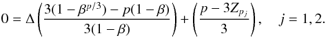 (3)Using Zp1, we can obtain an expression for Δ,
 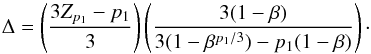 (4)By now writing Eq. (3) with Zp = Zp2, using Eq. (4) to replace Δ, do some re-ordering of terms, and abbreviating p1/ 3 ≡ a and p2/ 3 ≡ b, we end up with the following equation for β:
 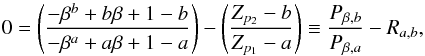 (5)or
(5)or 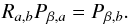 (6)The polynomial Pβ,x ≡ −βx + xβ + 1 − x, with x> 0 and β ∈ (0,1), is a monotonically decreasing (increasing) function for x< 1 (x> 1), as can be seen by taking the derivative of Pβ,x with respect to β and as illustrated in Fig. 1. Consequently, Eq. (6) has a unique solution, β, from which Δ can be recovered via Eq. (4). Thus Eq. (1) defines an exact one-to-one correspondence between pairs (Zp1,Zp2) and (β,Δ).
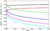 |
Fig. 1 Ratio of polynomials Pβ,b/Pβ,a, Eq. (5), (y-axis, shown as logarithm) for selected exponents a and b as function of β (x-axis). Colors indicate b/a = 2 (red), 4 (green), 5 (blue), 6 (magenta), 7 (cyan), all with a = p1/ 3 = 1/3, as well as b/a = 7/6 (black) with a = p1/ 3 = 6/3. |
Two more points deserve to be highlighted, with the help of Fig. 1. The ratio Pβ,b/Pβ,a = Ra,b is shown as a function of β for different a and b or, equivalently, p1 and p2. From the figure it can be taken that, first, largely different values of p1 and p2 are advantageous since they result in stronger stratification of β with respect to Ra,b = (Zp2 − b)/(Zp1 − a). The cyan curve in Fig. 1, which represents p1/p2 = 1/7, covers a wider range of values on the y-axis than the black curve (p1/p2 = 6/7). Secondly, the stratification is stronger for small β. Somewhat anticipating Sect. 2.2, we thus expect uncertainties in the Zp to be less important if Zp are available for largely different p and if they are associated with (yet to be determined) small values of β.
2.2. Uncertainty of Zp in the β-Δ-plane
2.2.1. Single Zp
From Eq. (4) it is clear that each Zp defines a curve in the β-Δ-plane. If Zp is derived from model data or observations, it will typically come with an uncertainty estimate, e.g. δZp/Zp ≤ 5%, with δ indicating the uncertainty. In the β-Δ-plane, this uncertainty range translates into an area around the Zp curve. An illustration is given in Fig. 2. The following points may be made.
One value of Zp (a line of constant Zp in the β-Δ-plane) is compatible with a (large) range of β and/or Δ that always includes Δ = 1 and β = 0. The range tends to be smaller for Zp associated with small β and large Δ (i.e. the lower right corner of β-Δ-plane). Uncertainties associated with Zp (5% in Fig. 2, white curves) augment the range, especially for p = 2 and p = 4, as well as for small Δ and large β (top left corner of the plane). Also apparent from Fig. 2 (or from taking the derivative with respect to Δ of Eq. (1)): for fixed β and p< 3 (p> 3), Zp is a monotonically increasing (decreasing) function of Δ. A similar statement holds for Zp as a function of β for fixed Δ.
In summary, we expect uncertainties in the Zp to be more of an issue if only low orders of p (up to about 4) are available and/or if the (yet to be determined) β is large.
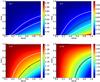 |
Fig. 2 Zp in the β-Δ-plane, role of p. Shown is Zp (color coded) for p = 1 (top left), p = 2 (top right), p = 4 (bottom left) and p = 10 (bottom right). For β = 1/3 and Δ = 2/3 (red dot), the curve of constant Zp (black) is shown, as well as curves of ± 5% different Zp (white). |
2.2.2. Multiple Zp
We now turn to multiple Zp and their associated uncertainty ranges δZp, and ask what area they define in the β-Δ-plane. An illustration is given in Fig. 3. Starting from one specific pair of β = 1/3 and Δ = 2/3 and computing Zp for p = 1,...,5 (left) or p = 1,...,7 (right), we show pairs of 5% perturbed Zp curves, i.e. 1.05·Zp and 0.95·Zp.
As can be seen, only a small fraction of the β-Δ-plane lies between all pairs of perturbed curves. Yet this area comprises a wide range of (β,Δ) values or co-dimensions. The 5% uncertainty in the Zp translates into a much larger uncertainty (in per cent) for β and Δ. Closer inspection reveals that the area is actually defined by only two sets of curves: those for p = 1 and p = 5 (left panel) or p = 7 (right panel). The latter area is smaller, which indicates that higher order structure functions constrain the problem of finding β and Δ from a set of Zp more strongly. Also apparent from Fig. 3 is the dominant role of the p = 1 curve for narrowing down the composite area between all curves. All this is in line with the expectation (see Sect. 2.1) that Zp for largely different p are advantageous for the determination of β and Δ.
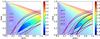 |
Fig. 3 Part of β-Δ-plane (color coded in co-dimension C = Δ/(1 − β), 0 <C< 3) within joint reach of (at most) 5% perturbed Zp, starting from Zp for Δ = 2/3 and β = 1/3 (red dot). Left panel: curves of 5% perturbed Zp values for p = 1 (white), p = 2 (blue), p = 4 (red), and p = 5 (green) and part of the β-Δ-plane enclosed by all of them. Right panel: same as left panel but also including p = 6 (purple) and p = 7 (black). |
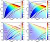 |
Fig. 4 Same as Fig. 3, left, but for β = Δ = 2/3 (top left), β = Δ = 1/3 (top right), β = 0.048 and Δ = 1/3 (bottom left), as well as and β = 0.048 and Δ = 2/3 (bottom right). |
The relevance of the overall location in the β-Δ-plane is illustrated in Fig. 4. Again, the area shown is contained within 5% perturbed Zp curves for two additional (β,Δ) pairs. As can be seen, smaller values of β (lower panels) result in smaller areas, independent of Δ. The crucial role of the p = 1 (white) and p = 5 (green) curves for confining the area persists. Table 1 gives a quantitative idea of the relevance of β, Δ, δZp, and pmax for the uncertainty range ± δC of the co-dimensions C. A small δC basically requires a small δZp, a large pmax, a small β, and a large Δ. The concrete numbers highlight the difficulty (or ill-posedness) of the problem. The situation is worse for larger β (bottom rows in Table 1) and better for smaller values of β (not shown).
We emphasize that the above considerations serve only as illustration. We looked at the area confined by a set of Zp ± δZp curves. We have not yet considered the problem of estimating best-fit βf, Δf, and thus Cf for a set of given Zp. Such a best-fit solution may lie outside the area considered here.
In summary, very accurate Zp are needed to derive reliable best estimates for β, Δ, and C, and smaller values of β help.
2.3. Best-fit βf and Δf from uncertain Zp
We now turn to our actual problem of interest: given a set of perturbed (uncertain)  , what are associated best-fit estimates for βf and Δf? Different techniques exist to cope with this kind of question (e.g. Najm 2009; Le Maître & Knio 2010). We use a simple Monte Carlo approach.
We start with a pair (β,Δ) and a maximum order pmax, then use Eq. (1) to obtain a set of Zp = Zp(β,Δ) for p = 1 to p = pmax. Each of these Zp we perturb randomly (uniformly distributed random numbers) by, at most, α%, which gives us a perturbed set of  . For this set of we then seek to find best-fit βf and Δf. In the following, we do not consider one set of , as would be the case in a real application (unless multiple time slices are available, see Sect. 3). Instead, we take a statistical view for the problem by looking at a large number (1000 to 100 000, see below) of randomly generated sets of perturbed . This enables us, in a statistical sense, to relate the accuracy of the with the accuracy of the fitted parameters. Our approach leaves us with two free parameters, the uncertainty α and the maximum order pmax.
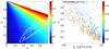 |
Fig. 5 Best-fit βf and Δf from 5% perturbed Zp. Left: 2D histogram (contours, log10, spacing 0.5, spanning three orders of magnitude) of best-fit β-Δ-values from 100 000 perturbed data sets. We note that the 2D histogram shows two peak values (indicated by cyan dots), none of them co-located with the unperturbed (β = 1/3,Δ = 2/3) pair (red dot). Right: underestimation of Z5 favors Δf = 1. Shown is, for a subset of 1000 perturbed data sets, Δf as function of |


Illustration of range δC of co-dimension C for given order p and uncertainty δZp of structure functions for two β-Δ pairs.
2.3.1. Minimization of least square error in Zp
A straightforward way to determine best-fit βf and Δf for any given set of , p = 1,...,pmax is to minimize ![\begin{equation} \sum_{p=1}^{p_{\mathrm{max}}} [\tilde{Z}_{p} - Z_{p}(\beta_{\mathrm{f}},\Delta_{\mathrm{f}})]^{2} \label{eq:to_minimize} \end{equation}](/articles/aa/full_html/2016/03/aa27148-15/aa27148-15-eq149.png) (7)over the β-Δ-plane. To find the minimum, we compare the with pre-computed values Zp(β,Δ) on a fine β-Δ-grid (β,Δ ∈ (0,1); grid-spacing 0.002). The associated co-dimension is given by Cf = Δf/ (1 − βf).
(7)over the β-Δ-plane. To find the minimum, we compare the with pre-computed values Zp(β,Δ) on a fine β-Δ-grid (β,Δ ∈ (0,1); grid-spacing 0.002). The associated co-dimension is given by Cf = Δf/ (1 − βf).
To capture the range of potential outcomes for a range of similarly perturbed data sets , we produced 100 000 perturbed data sets, for each of which we determined βf and Δf. For initial values (β,Δ) = (1/3,2/3) and (at most) 5% perturbed Zp for p = 1,...,5, the result is summarized in Fig. 5.
Shown in the left panel of Fig. 5 is a 2D histogram (contours) of our 100 000 best-fit (βf,Δf) pairs. Two points are noteworthy. First, the overall area defined by the histogram is similar to the area in Fig. 3, left panel. This is remarkable since the area in Fig. 3 is strictly defined by the 5% uncertainty of the Zp, whereas the area in Fig. 5 is defined through a minimization problem. Second, the 2D histogram has an interior structure with two peaks, around (β,Δ) = (0.1,0.4) or C = 0.4 and (β,Δ) = (0.45,1.0) or C = 1.8 (cyan dots). None of them is co-located with the initial, unperturbed (β,Δ) = (1/3,2/3) pair (red dot, C = 1).
Three questions come to mind. Where do the two peaks in the 2D histogram come from? Do other (β,Δ) pairs result in a qualitatively different picture? Can the minimization procedure be improved to better recover the initial, unperturbed (β,Δ) pair? We address the first two questions in the following while postponing the third question for Sect. 2.3.2.
The existence and location of the two peaks can be understood, at least qualitatively, from two observations. First, minimization via Eq. (7) gives more weight to larger p, as they are associated with larger values of Zp. Roughly speaking, the best-fit (βf,Δf) pair tends to lie on or close to the curve defined by  . Moving away from that curve results in a large penalty in the form of a large contribution to the sum in Eq. (7). Second, this translates the minimization problem into the question of where the curves for p< 5 come closest to the curve defined by . For illustration, we consider two extreme values of . To stay on the lower green curve in the left panel of Fig. 3, (
 ) and, at the same time, be as close as possible to any of the white curves (p = 1) results in a (βf,Δf) pair to the right, at Δf ≈ 1. By contrast, the upper green curve (105% of the exact Z5 curve) only comes closest to (intersects) any white curve between 95% Z1 and 105% Z1 in a region further to the left. Clearly, the full problem is more intricate, with also curves for Z2 and Z4, and the Z5 curve not necessarily adopting one of its two extreme values. Nevertheless, Fig. 5, right panel, suggests the full data to be in line with the above reasoning. For 1000 randomly picked data sets from the left panel, we show Δf as a function of
  , with Z5 the exact value. Colors indicate
  . As can be seen, Δf = 1 indeed tends to be associated with small and small
  (lower green and upper white curve in Fig. 3, left panel). Particularly low values of Δf (e.g. Δf ≈ 0.4) tend to occur for large and any (upper green curve and any white curve in Fig. 3, left panel).
Concerning other initial values (other exact (β,Δ) pairs), a similar situation arises in the sense that double peaked histograms emerge. Details depend, however, on the concrete values of β and Δ, on the assumed uncertainty (5% or more/less), and on pmax. An illustration is given in Fig. 6, by means of 1D histograms of Cf = Δf/ (1 − βf). These 1D histograms are less intricate than the 2D histogram in Fig. 5, left, yet still capture the essentials. We show histograms for Δ = 2/3 and different values of β ∈ [0.0476,2/3] (corresponding to C ∈ [0.7,2]) and accuracies between 0.1% and 20%. Five points may be made. First, the double-peaked structure that is apparent in the β-Δ plane in Fig. 5 re-appears as a double peak in the 1D Cf-histograms of Fig. 6 (panel in row three, column three). Second, the double-peak vanishes as β and the uncertainty both become small (lower left corner of the figure). For the same uncertainty, the double-peak exists for large β but not for small β (third row in Fig. 6). For the same β, the double-peak exists for large uncertainties but not for small ones (second column of Fig. 6). Third, going to really small values of β and the uncertainty, the histogram becomes symmetric with one central peak. Fourth, only for these really small values is the co-dimension of the initially prescribed (β,Δ) pair (show in red) co-located with the peak of the histogram. Fifth, for β = Δ = 2/3 (right column) the histogram peaks at Cf = 3 instead of C = 2, unless the accuracy is really high (0.1%, last row). This is understandable from the arguments presented above, with regards to the origin of the two peaks in the 2D histogram in Fig. 5, and from looking at the green (p = 5) and white (p = 1) curves in Fig. 4, upper left panel.
In summary, unless both, δZp and β are small, best-fit values will preferentially reside in either one of the two peaks of the histograms in Figs. 5 or 6 instead of merely scattering around the correct solution, as in Fig. 6, lower left panel.
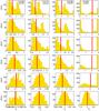 |
Fig. 6 Role of β (columns) and accuracy (rows) of associated Zp, for fixed Δ = 2/3. Shown are PDFs (y-axis) of Cf (x-axis), 1000 random data sets, powers p = 1,...,5 for β = 0.0476 (first column), β = 0.17 (second column), β = 1/3 (third column), and β = 2/3 (fourth column). Corresponding exact co-dimensions (red lines) are, from left to right: C = 0.7, C = 0.8, C = 1, and C = 2. Individual rows from top to bottom contain accuracies of 20%, 10%, 5%, 2%, 0.5%, and 0.1%. As can be seen, the larger β, the more severe are the consequences of inaccuracies in the Zp. Histograms in the upper right (large β, low accuracy of the Zp) look worst. We note that axis ranges differ among panels, to best capture the shape of each histogram. |
2.3.2. Alternative ways to obtain best-fit βf and Δf
A number of ideas come to mind on how one may improve the best-fit approach detailed in Sect. 2.3.1.
Recalling the findings in Sect. 2.2.1, including higher values of p in the best-fit estimate should improve the situation. From Fig. 7 it can be taken that this is indeed the case, at least for the example shown (β = 1/3, Δ = 2/3, accuracy of 5%). However, the improvement may be regarded as rather modest. Going from p = 5 to p = 10, as is illustrated in the figure, has about the same effect as staying with p = 5 but going from an accuracy of 5% to an accuracy of 2%. From a practical point of view it also seems questionable whether high order structure functions can meet the accuracy requirements. In numerical simulations, higher order structure functions are probably more prone to the bottleneck effect (Dobler et al. 2003; Kritsuk et al. 2007a).
Another way to improve the situation could be to go to weighted root mean squares instead of the unweighted sum in Eq. (7). Hopefully this breaks the dominant role of the highest order Zp available (see Sect. 2.3.1) and, ultimately, leads to more accurate best-fit βf and Δf. Two weightings come to mind. On the one hand, weights proportional to the inverse of the Zp with the goal of giving equal weight to each term in the sum, thus reducing the “overweight” of larger p in the sum. On the other hand, we could try to give more weight to p terms with a higher accuracy (smaller δZp). Corresponding information may be available, e.g. from the numerical determination of the Zp. We tried both ideas but neither choice of weights decidedly improved the best-fit values. Weighting tends to change the relative height of the two peaks in the double peaked histograms of Fig. 6, but it does not get rid of the double peaked structure.
We interpret this finding in the following way. First, there are likely always several Zp that do not have their exact values and thus draw the solution in different directions, away from its exact value. Second, the different curve shapes are important so that, even for weighted sums, the terms p = 1 and p = pmax are of crucial importance for the overall fit.
In summary, none of the above alternative ways of fitting simultaneously for β and Δ provides clearly superior results to what can be obtained from the straightforward minimization of Eq. (7). We conclude that, for successful two-parameter fits of β and Δ, highly accurate Zp are a must. A quantitative estimate of “highly accurate”is given in the next section.
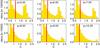 |
Fig. 7 Role of higher order moments. Inclusion of higher order ESS scaling exponents (from p = 5, top left, to p = 10, bottom right) gradually reduces the erroneous peak in the best-fit co-dimension (around Cf = 2.5). Shown are PDFs of Cf for at most 5% perturbed Zp values (100 000 random data sets) and exact pair (β = 1/3,Δ = 2/3). Spacing of the β-Δ-grid for fitting is 0.002. |
2.3.3. Required accuracy of Zp for “good” best-fit βf and Δf
We now ask how accurate the Zp have to be in order to reach a prescribed accuracy of Cf = Δf/ (1 − βf) via fitting βf and Δf.
We formulate our accuracy goal in terms of only Cf, since we illustrated in Sect. 2.3.1 that a single peaked and roughly symmetric distribution of Cf goes hand in hand with high accuracy, not only of Cf but also of the underlying two parameter fit, βf and Δf. If the latter is not accurate enough, a double peaked distribution for Cf results. We find, as a rule of thumb, a single peak distribution if 2/3 of all Cf lie within 10% or better of the exact C. We use Eq. (7) for the two parameter fit, as the more elaborate attempts of Sect. 2.3.2 gave no decidedly better results. As theoretical arguments suggest Δ = 2/3 or larger (Dubrulle 1994; Schmidt et al. 2008), we concentrate on that part of the β-Δ-plane.
In practical terms, we define a grid of exact pairs (β,Δ) via a (nearly) equidistant grid of C = 0.4,...,2 and Δ = 0.7,...,0.99 plus, in addition, Δ = 2/3. We equally define some fixed levels of perturbations: δZp/Zp (in %) ∈ [0.05,0.1,0.2,0.5,1,2,5,10,15,20]. For each exact pair and each perturbation, we created 1000 perturbed sets of , p = 1,...,5 (see Sect. 2.3). Each perturbed set is fitted via Eq. (7). For each initial pair (β, Δ) and for each prescribed δZp/Zp this yields 1000 fitted pairs (βf,Δf) and derived co-dimensions Cf. These can, in principle, be arranged in histograms, as in Fig. 6. Finally, we identify the largest δZp/Zp for which 2/3 of all Cf lie within the demanded accuracy of the exact, initial C.
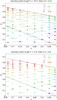 |
Fig. 8 Required accuracy (color coding) of perturbed Zp, p = 1,...,5, such that for at least 2/3 of the best-fit pairs (βf, Δf) the associated Cf are within 10% (top) or 5% (bottom) of the C associated with the initial, unperturbed (β, Δ) pair. As can be seen, the required accuracy depends crucially on the location within the β-Δ plane. Gray lines indicate the range within which 2/3 of the actual βf (vertical direction) and Δf (horizontal direction) lie. Black lines indicate constant C = 1 (lower line) and C = 2 (upper line). For details see text. |
Figure 8 illustrates the result. Obviously, the accuracy of the (colored squares, in %) that is needed to get at least 2/3 of best-fit Cf to lie within 10% (top panel) or 5% (bottom panel) of the exact (initial) C depends on the position within the β-Δ-plane. In the lower right parts, δZp/Zp ≥ 1% is sufficient to get 10% accurate Cf, and δZp/Zp ≥ 0.5% yields 5% accurate Cf. By contrast, in the upper left parts of the plane (β ≥ 0.5) one needs δZp/Zp ≤ 0.1% to get 10% accurate Cf. Gray lines in Fig. 8 (for clarity only shown for a subset of the colored squares) indicate the range within which at least 2/3 of the actually fitted βf and Δf lie. The range is larger for Δ (horizontal lines) than for β (vertical lines). This is plausible from Fig. 4, from the area confined by multiple Zp curves. Repeating Fig. 8 but demanding 10% accuracy for Δf instead of Cf yields a similar pattern in the β-Δ-plane (not shown), while demanding 10% accuracy for βf gives a much more homogeneous pattern (0.2% to 0.5% accuracy for , not shown).
For highly compressible turbulence, best-fit βf and Δf are expected to lie in the lower part of the β-Δ-plane in Fig. 8, roughly β ≤ 1/3 and Δ ≥ 2/3 (Boldyrev 2002; Padoan et al. 2004; Pan et al. 2009). Here, accuracies of 0.5%, 0.1%, and 0.05% for the translate into accuracies of 10%, 2%, and 1% for βf and Δf (not shown). Fits of similar quality require much more accurate in the mildly compressible regime, where β> 1/3 (upper part of panels in Fig. 8) and ultimately β = 2/3 in the incompressible limit. We note that in practical applications, best-fit values may be further improved by combining, for example, data from different time slices (Pan et al. 2009).
In summary, a 2% (1%) accurate simultaneous fit for βf and Δf should be possible in the highly compressible regime if the Zp are 0.1% (0.05%) accurate. If no satisfying fit is possible for such Zp, this may indicate that the model is not applicable to the turbulence data under examination.
3. Discussion
We address three topics. First, can the necessary accuracy for the Zp be met in practical applications? Second, if we had this type of accurate simulation data, what could be learned about the hierarchical structure model and its applicability or non-applicability to driven, isothermal, supersonic turbulence in a 3D periodic box? Third, we want to briefly revisit the frequently used one parameter fits.
We start with the question whether 0.1% or even 0.05% accurate Zp for p = 1,...,5 are achievable, as are needed to get 2% (1%) accurate fits for β and Δ. The answer is probably yes, at least in the context of 3D periodic box simulations. Schmidt et al. (2008) estimate the accuracy of their Zp, p = 1,...,5, to 1% (3D box simulations, 10243). Kritsuk et al. (2007a) estimate 1% accuracy or better for absolute scaling exponents ζp, p = 1,...,3 (3D box simulations, 10243). Meanwhile, 3D box simulations with 40963 exist (e.g. Federrath 2013; Beresnyak 2014). A first order estimate suggests the four times better resolution to translate into four times (first order scheme) or 16 times (second order scheme) more accurate structure functions, thus accuracies of 0.25% or even 0.0625%. Moreover, if the accuracy of the Zp is good enough to avoid double peaked histograms as in Fig. 6, accuracy may be further enhanced by exploring multiple time slices. Pan et al. (2009; 3D box simulations, 10243) used data from nine time slices for their two parameter fit. Their work is comparable although they rely on dissipation rates instead of velocity structure functions, since the involved scaling exponents (τp for the dissipation rate) are structurally similar according to Kolmogorov’s refined similarity hypothesis (Kolmogorov 1962), ζp = p/ 3 + τp/ 3. The tests we carried out using ratios of τp instead of ζp indeed show a similar behavior. From the quality of their fit and based on our results, we estimate their τp to be about 1% accurate, which is plausible given their numerical resolution. A reliable two parameter fit to 3D periodic box data of highly supersonic turbulence that is based on velocity structure functions thus appears feasible with today’s data.
What could be learned from better simulation data (40963 or better) and associated, more accurate Zp? Each Zp defines a curve with associated uncertainty in the β-Δ plane, the curves for different p may or may not intersect to within uncertainties. If they intersect, the model by She & Leveque (1994) may indeed carry over to highly compressible turbulence. It is then interesting to see whether the fitted range for Δ, currently estimated as (0.67−0.78) by Pan et al. (2009), remains compatible with Δ = 2/3, the value tacitly assumed in a large body of literature. It is also interesting to check whether β = 1/3, as theoretically anticipated by Boldyrev (2002). If indeed (β,Δ) = (1/3,2/3), results from one parameter fits that quantify the transition to incompressible turbulence (β = Δ = 2/3) with decreasing Mach number likely apply (Padoan et al. 2004). If Δ ≠ 2/3, two parameter fits for β and Δ would also be needed in the mildly compressible regime. However, the analysis in Sect. 2.3.3 suggests that these kind of fits are likely beyond reach of today’s computer resources.
The latter of the above cases, where the Zp curves do not intersect to within their uncertainty, would imply that the model by She & Leveque (1994) does not carry over to 3D periodic box simulations of driven, isothermal, highly compressible turbulence. A simple reason here could be that theoretical results are based on the assumption of an infinite Reynolds number, a criterion clearly violated by numerical simulations. More importantly, She & Waymire (1995) already pointed out that there is no reason why only one dimension should be associated with the most dissipative structure. They argued that in such a large portion of space as is typically analyzed, a variety of most dissipative structures may co-exist with different co-dimensions. Hopkins (2013) suggests a slightly different model based on work by Castaing (1996), which is more compatible with not strictly log-normal density PDFs as observed in isothermal supersonic turbulence. Finally, yet other models exist, (e.g. via multifractals Macek et al. 2011; Zybin & Sirota 2013), as well as other perspectives on the fractal character of a turbulent medium (see e.g. Kritsuk et al. 2007a).
Lastly, we briefly come back to the one parameter fits that are often used in the literature. Fixing the value of Δ by hand greatly reduces the impact of uncertainties in the Zp on the accuracy of the estimated best-fit co-dimension Cf. Folini et al. (2014) found 5% uncertain Zp, p = 1,...,5, to translate into roughly 10% uncertainty of the Cf for fixed Δ = 2/3. Fig. 3 offers a qualitative understanding of this reduced “error propagation”, which suggests some sensitivity to the specific location in the β-Δ-plane, and indicates that fixing C or β instead of Δ has a similar effect. Fixing β seems questionable at first sight since there is, to our knowledge, little theoretical understanding of what numerical value β might have (see e.g. Dubrulle 1994). On the other hand, She et al. (2001) presented a theoretical framework that allows for an independent determination of only β from the relative scaling exponents Zp (see also Hily-Blant et al. (2008), their Appendix A3). One could thus imagine breaking the two parameter fit for β and Δ into a two step procedure: first, fix the value of β, then use this value and do a one parameter fit for Δ. Hopefully this type of a two step approach is more robust against uncertainties in the Zp, but this question is beyond the scope of the current paper and we are unaware of corresponding attempts in the literature.
4. Summary and conclusions
This study was motivated by the overarching question of whether or not the random cascade model (She & Leveque 1994; Dubrulle 1994; She & Waymire 1995; Boldyrev 2002) applies to simulation data of highly compressible isothermal turbulence and, if so, with what parameter values for β and Δ. If applicable, the model offers a theoretical link between observable properties of the turbulence, namely ratios Zp of scaling exponents of the structure functions, and non-observable turbulence characteristics, for example the dimension D of the most dissipative structures. To date, applicability of the model is assumed in much of the literature with Δ = 2/3, a value just marginally compatible with simulation-based best estimates (Pan et al. 2009): Δ = 0.71 with an uncertainty range Δ ∈ (0.67,0.78).
We examine how uncertainties in the Zp translate into uncertainties of best-fit β-Δ-pairs and discuss what best-fits, consequently, seem achievable with today’s computer resources. A Monte Carlo approach is used to mimic actual simulation data. The results can be summarized in six main points.
-
Simultaneous fitting of β and Δ to sets of substantially (5%) perturbed (uncertain) Zp yields a “double peaked ridge” of best-fit values in the β-Δ plane. None of the two peaks is co-located with the initial (β,Δ) pair.
-
The highest and lowest order p are particularly relevant for simultaneous fitting of β and Δ. A somewhat optimal choice is p = 1,...,5. Yet higher order structure functions add comparatively little to the quality of the fit, while they tend to be afflicted with larger uncertainties in real applications.
-
A simultaneous, 2% (1%) accurate fit of β and Δ should be possible if the Zp, p = 1,...,5, are 0.1% (0.05%) accurate and if the (yet to be determined) value of β is about 1/3 or less.
-
Applicability of the model thus may be best tested in the highly compressible regime, where β ≈ 1 /3 is expected, and not in the mildly compressible regime where β ultimately must approach its incompressible value of 2/3.
-
We argue that today’s computer resources likely allow to reach this accuracy. Existing simulations of 40963 (Federrath 2013; Beresnyak 2014) probably allow for at least 2%, possibly 1% accurate estimates of β and Δ.
-
Should the ambiguity in the determination of β and Δ persist despite such highly accurate Zp, this may indicate that the notion of She & Waymire (1995; β and Δ take a continuum of values) or Hopkins (2013; a different model for the statistics of the inertial range) is correct or that yet a different turbulence model is needed in this regime.
Acknowledgments
R.W. and D.F. acknowledge support from the French National Program for High Energies PNHE. We acknowledge support from the Pôle Scientifique de Modélisation Numérique (PSMN), from the Grand Equipement National de Calcul Intensif (GENCI), project number x2014046960, and from the European Research Council through grant ERC-AdG No. 320478-TOFU.
References
- Benzi, R., Ciliberto, S., Tripiccione, R., et al. 1993, Phys. Rev. E, 48, 29 [Google Scholar]
- Beresnyak, A. 2014, ApJ, 784, L20 [NASA ADS] [CrossRef] [Google Scholar]
- Boldyrev, S. 2002, ApJ, 569, 841 [NASA ADS] [CrossRef] [Google Scholar]
- Boldyrev, S., Nordlund, Å., & Padoan, P. 2002, Phys. Rev. Lett., 89, 031102 [NASA ADS] [CrossRef] [Google Scholar]
- Castaing, B. 1996, J. Phys. II, 6, 105 [Google Scholar]
- Chabrier, G., & Hennebelle, P. 2011, A&A, 534, A106 [NASA ADS] [CrossRef] [EDP Sciences] [Google Scholar]
- Dobler, W., Haugen, N. E., Yousef, T. A., & Brandenburg, A. 2003, Phys. Rev. E, 68, 026304 [NASA ADS] [CrossRef] [Google Scholar]
- Dubrulle, B. 1994, Phys. Rev. Lett., 73, 959 [NASA ADS] [CrossRef] [PubMed] [Google Scholar]
- Federrath, C. 2013, MNRAS, 436, 1245 [NASA ADS] [CrossRef] [Google Scholar]
- Federrath, C., & Klessen, R. S. 2012, ApJ, 761, 156 [NASA ADS] [CrossRef] [Google Scholar]
- Folini, D., Walder, R., & Favre, J. M. 2014, A&A, 562, A112 [NASA ADS] [CrossRef] [EDP Sciences] [Google Scholar]
- Gustafsson, M., Brandenburg, A., Lemaire, J. L., & Field, D. 2006, A&A, 454, 815 [NASA ADS] [CrossRef] [EDP Sciences] [Google Scholar]
- Hennebelle, P., & Chabrier, G. 2008, ApJ, 684, 395 [NASA ADS] [CrossRef] [Google Scholar]
- Hily-Blant, P., Falgarone, E., & Pety, J. 2008, A&A, 481, 367 [NASA ADS] [CrossRef] [EDP Sciences] [Google Scholar]
- Hobbs, A., Nayakshin, S., Power, C., & King, A. 2011, MNRAS, 413, 2633 [NASA ADS] [CrossRef] [Google Scholar]
- Hopkins, P. F. 2013, MNRAS, 430, 1880 [NASA ADS] [CrossRef] [Google Scholar]
- Kolmogorov, A. N. 1962, J. Fluid Mech., 13, 82 [NASA ADS] [CrossRef] [Google Scholar]
- Kritsuk, A. G., Norman, M. L., Padoan, P., & Wagner, R. 2007a, ApJ, 665, 416 [NASA ADS] [CrossRef] [Google Scholar]
- Kritsuk, A. G., Padoan, P., Wagner, R., & Norman, M. L. 2007b, in Turbulence and Nonlinear Processes in Astrophysical Plasmas, eds. D. Shaikh, & G. P. Zank, AIP Conf. Ser., 932, 393 [Google Scholar]
- Kritsuk, A. G., Lee, C. T., & Norman, M. L. 2013, MNRAS, 436, 3247 [NASA ADS] [CrossRef] [Google Scholar]
- Lazar, A., Nakar, E., & Piran, T. 2009, ApJ, 695, L10 [NASA ADS] [CrossRef] [Google Scholar]
- Le Maître, O. P., & Knio, O. M. 2010, Spectral Methods for Uncertainty Quantification (Springer) [Google Scholar]
- Macek, W. M., Wawrzaszek, A., & Carbone, V. 2011, Geophys. Res. Lett., 38, 19103 [NASA ADS] [CrossRef] [Google Scholar]
- Najm, H. N. 2009, Ann. Rev. Fluid Mech., 41, 35 [NASA ADS] [CrossRef] [Google Scholar]
- Narayan, R., & Kumar, P. 2009, MNRAS, 394, L117 [NASA ADS] [CrossRef] [Google Scholar]
- Padoan, P., Jimenez, R., Nordlund, Å., & Boldyrev, S. 2004, Phys. Rev. Lett., 92, 191102 [NASA ADS] [CrossRef] [PubMed] [Google Scholar]
- Padoan, P., Haugbølle, T., & Nordlund, Å. 2012, ApJ, 759, L27 [NASA ADS] [CrossRef] [MathSciNet] [Google Scholar]
- Pan, L., Padoan, P., & Kritsuk, A. G. 2009, Phys. Rev. Lett., 102, 034501 [NASA ADS] [CrossRef] [PubMed] [Google Scholar]
- Schmidt, W., Federrath, C., & Klessen, R. 2008, Phys. Rev. Lett., 101, 194505 [NASA ADS] [CrossRef] [PubMed] [Google Scholar]
- Schmidt, W., Federrath, C., Hupp, M., Kern, S., & Niemeyer, J. C. 2009, A&A, 494, 127 [NASA ADS] [CrossRef] [EDP Sciences] [Google Scholar]
- She, Z.-S., & Leveque, E. 1994, Phys. Rev. Lett., 72, 336 [Google Scholar]
- She, Z.-S., & Waymire, E. C. 1995, Phys. Rev. Lett., 74, 262 [NASA ADS] [CrossRef] [PubMed] [Google Scholar]
- She, Z.-S., & Zhang, Z.-X. 2009, Acta Mech. Sin., 25, 279 [NASA ADS] [CrossRef] [Google Scholar]
- She, Z.-S., Ren, K., Lewis, G. S., & Swinney, H. L. 2001, Phys. Rev. E, 64, 016308 [NASA ADS] [CrossRef] [Google Scholar]
- Walder, R., Folini, D., & Shore, S. N. 2008, A&A, 484, L9 [NASA ADS] [CrossRef] [EDP Sciences] [Google Scholar]
- Zybin, K. P., & Sirota, V. A. 2013, Phys. Rev. E, 88, 043017 [NASA ADS] [CrossRef] [Google Scholar]
All Tables
Illustration of range δC of co-dimension C for given order p and uncertainty δZp of structure functions for two β-Δ pairs.
All Figures
|
Fig. 1 Ratio of polynomials Pβ,b/Pβ,a, Eq. (5), (y-axis, shown as logarithm) for selected exponents a and b as function of β (x-axis). Colors indicate b/a = 2 (red), 4 (green), 5 (blue), 6 (magenta), 7 (cyan), all with a = p1/ 3 = 1/3, as well as b/a = 7/6 (black) with a = p1/ 3 = 6/3. |
| In the text | |
|
Fig. 2 Zp in the β-Δ-plane, role of p. Shown is Zp (color coded) for p = 1 (top left), p = 2 (top right), p = 4 (bottom left) and p = 10 (bottom right). For β = 1/3 and Δ = 2/3 (red dot), the curve of constant Zp (black) is shown, as well as curves of ± 5% different Zp (white). |
| In the text | |
|
Fig. 3 Part of β-Δ-plane (color coded in co-dimension C = Δ/(1 − β), 0 <C< 3) within joint reach of (at most) 5% perturbed Zp, starting from Zp for Δ = 2/3 and β = 1/3 (red dot). Left panel: curves of 5% perturbed Zp values for p = 1 (white), p = 2 (blue), p = 4 (red), and p = 5 (green) and part of the β-Δ-plane enclosed by all of them. Right panel: same as left panel but also including p = 6 (purple) and p = 7 (black). |
| In the text | |
|
Fig. 4 Same as Fig. 3, left, but for β = Δ = 2/3 (top left), β = Δ = 1/3 (top right), β = 0.048 and Δ = 1/3 (bottom left), as well as and β = 0.048 and Δ = 2/3 (bottom right). |
| In the text | |
|
Fig. 5 Best-fit βf and Δf from 5% perturbed Zp. Left: 2D histogram (contours, log10, spacing 0.5, spanning three orders of magnitude) of best-fit β-Δ-values from 100 000 perturbed data sets. We note that the 2D histogram shows two peak values (indicated by cyan dots), none of them co-located with the unperturbed (β = 1/3,Δ = 2/3) pair (red dot). Right: underestimation of Z5 favors Δf = 1. Shown is, for a subset of 1000 perturbed data sets, Δf as function of |
| In the text | |
|
Fig. 6 Role of β (columns) and accuracy (rows) of associated Zp, for fixed Δ = 2/3. Shown are PDFs (y-axis) of Cf (x-axis), 1000 random data sets, powers p = 1,...,5 for β = 0.0476 (first column), β = 0.17 (second column), β = 1/3 (third column), and β = 2/3 (fourth column). Corresponding exact co-dimensions (red lines) are, from left to right: C = 0.7, C = 0.8, C = 1, and C = 2. Individual rows from top to bottom contain accuracies of 20%, 10%, 5%, 2%, 0.5%, and 0.1%. As can be seen, the larger β, the more severe are the consequences of inaccuracies in the Zp. Histograms in the upper right (large β, low accuracy of the Zp) look worst. We note that axis ranges differ among panels, to best capture the shape of each histogram. |
| In the text | |
|
Fig. 7 Role of higher order moments. Inclusion of higher order ESS scaling exponents (from p = 5, top left, to p = 10, bottom right) gradually reduces the erroneous peak in the best-fit co-dimension (around Cf = 2.5). Shown are PDFs of Cf for at most 5% perturbed Zp values (100 000 random data sets) and exact pair (β = 1/3,Δ = 2/3). Spacing of the β-Δ-grid for fitting is 0.002. |
| In the text | |
|
Fig. 8 Required accuracy (color coding) of perturbed Zp, p = 1,...,5, such that for at least 2/3 of the best-fit pairs (βf, Δf) the associated Cf are within 10% (top) or 5% (bottom) of the C associated with the initial, unperturbed (β, Δ) pair. As can be seen, the required accuracy depends crucially on the location within the β-Δ plane. Gray lines indicate the range within which 2/3 of the actual βf (vertical direction) and Δf (horizontal direction) lie. Black lines indicate constant C = 1 (lower line) and C = 2 (upper line). For details see text. |
| In the text | |
Current usage metrics show cumulative count of Article Views (full-text article views including HTML views, PDF and ePub downloads, according to the available data) and Abstracts Views on Vision4Press platform.
Data correspond to usage on the plateform after 2015. The current usage metrics is available 48-96 hours after online publication and is updated daily on week days.
Initial download of the metrics may take a while.