| Issue |
A&A
Volume 587, March 2016
|
|
|---|---|---|
| Article Number | A148 | |
| Number of page(s) | 20 | |
| Section | Interstellar and circumstellar matter | |
| DOI | https://doi.org/10.1051/0004-6361/201527001 | |
| Published online | 04 March 2016 | |
The connection between supernova remnants and the Galactic magnetic field: A global radio study of the axisymmetric sample
1 Dept of Physics and Astronomy, University of Manitoba, Winnipeg, R3T 2N2, Canada
e-mail: This email address is being protected from spambots. You need JavaScript enabled to view it.
; This email address is being protected from spambots. You need JavaScript enabled to view it.
2 Université de Toulouse, UPS-OMP, IRAP, 31028 Toulouse, France
3 CNRS, IRAP, 9 Av. colonel Roche, BP 44346, 31028 Toulouse Cedex 4, France
4 National Research Council, Herzberg Programs in Astronomy & Astrophysics, Dominion Radio Astrophysical Observatory, PO Box 248, Penticton, V2A 6J9, Canada
5 Dept of Physics & Astronomy, Brandon University, Brandon R7A 6A9, Canada
Received: 20 July 2015
Accepted: 28 October 2015
Abstract
The study of supernova remnants (SNRs) is fundamental to understanding the chemical enrichment and magnetism in galaxies, including our own Milky Way. In an effort to understand the connection between the morphology of SNRs and the Galactic magnetic field (GMF), we have examined the radio images of all known SNRs in our Galaxy and compiled a large sample that have an axisymmetric morphology, which we define to mean SNRs with a bilateral or barrel-shaped morphology, in addition to one-sided shells. We selected the cleanest examples and model each of these at their appropriate Galactic position using two GMF models, one of which includes a vertical halo component, and another that is oriented entirely parallel to the plane. Since the magnitude and relative orientation of the magnetic field changes with distance from the sun, we analyze a range of distances, from 0.5 to 10 kpc in each case. Using a physically motivated model of an SNR expanding into an ambient GMF that includes a vertical halo component, we find it is able to reproduce observed morphologies of many SNRs in our sample. These results strongly support the presence of an off-plane, vertical component to the GMF, and the importance of the Galactic field on SNR morphology. Our approach also provides a potentially new method for determining distances to SNRs, or conversely, distances to features in the large-scale GMF if SNR distances are known.
Key words: ISM: supernova remnants / ISM: magnetic fields / radio continuum: ISM
Canada Research Chair.
© ESO, 2016
1. Introduction
Supernova explosions are some of the most significant and transformative events in our Universe. Understanding supernova remnants (SNRs), the remains of these explosions, is fundamental to understanding the chemical enrichment and magnetism in galaxies, including our own Milky Way. Shaped by energetic supernova explosions in the circumstellar medium (CSM) or the interstellar medium (ISM), SNRs provide a powerful tool to study the intrinsic properties of the explosion and the environment in which they are expanding. Since the radio emission from SNRs originates primarily from synchrotron radiation of relativistic particles in the presence of compressed magnetic fields, radio observations are particularly useful for probing their magnetic fields and connection to the Galaxy (see Reynolds et al. 2012 and references therein for a review).
A subclass of SNRs, referred to as the bilateral or barrel-shaped, which are characterized by a symmetry axis (also referred to as “axisymmetric” by some authors) that divides two opposing limbs of radio emission, have a distinctive morphology. Several authors have proposed a connection between this characteristic morphology and the Galactic magnetic field (GMF) and cosmic ray density. A historical view, first proposed by van der Laan (1962, see also Whiteoak & Gardner 1968, is that an SNR that is expanding in a relatively uniform magnetic field will sweep up and compress the field where the expansion is perpendicular to the field lines. Regions where the field increases produce higher intensity radio synchrotron emission and thus are responsible for the appearance of the bright limbs. Kesteven & Caswell (1987) suggested that the majority of SNRs would have this barrel shape and that distorted remnants were the result of an inhomogeneous ISM. Further to this, Orlando et al. (2007) show that asymmetries in bilateral SNRs can be explained by gradients of ambient density or magnetic field strength. Thus we consider unilateral SNRs (ones observed with a single well-defined limb, e.g., G024.7–00.6, or ones having two limbs with one much brighter than the other, e.g., G127.1+00.5) as having their origin from the same processes as the bilateral type. We therefore include as axisymmetric those objects where we can draw a line across the image, to separate two approximately symmetric structural forms, even if the intensity of those forms differs. As such, we include SNRs where the structure on one side of the symmetry axis is quite faint.
Gaensler (1998) pointed out that some early studies (Shaver 1982; Manchester 1987; Leckband et al. 1989; Whiteoak & Green 1996) concluded that there was no clear relationship between the angle of the axis of bilateral symmetry and the Galactic plane (hereafter called the bilateral axis angle, ψ). Gaensler’s analysis used a tightly constrained sample of bilateral SNRs to conclude that there was a significant tendency for the bilateral axes of these SNRs to be aligned with the Galactic plane. However, even with a somewhat restrictive selection criterion, which constrained the sample to 17 bilateral SNRs, some are still significantly misaligned. One prime example is G327.6+14.6 (SN1006), which is perhaps the cleanest and most distinct example of an SNR with bilateral symmetry, and which is rotated almost 90° to the direction of the Galactic plane.
These previous studies were selective in their sample of axisymmetric SNRs, and in the modeling they did not account for an off-plane, vertical component of the Galactic field. The work reported here scrutinizes radio images of all known SNRs in our Galaxy, providing a more objective and complete sample of axisymmetric SNRs, and makes use of the most comprehensive GMF model to date. In Sect. 2, we summarize the current understanding of the magnetic field in SNRs (Sect. 2.1) and the Galaxy (Sect. 2.2). In Sect. 3, we discuss previous modeling of bilateral SNRs including the distribution of cosmic-ray electrons (CREs), which is another factor in determining the morphology of SNRs. Our process for selecting the sample of SNRs used for this study is discussed in Sect. 4. In Sect. 5, we describe our modeling, including an outline of the modeling procedure (Sect. 5.1) and the details of our SNR model (Sect. 5.2). We compare our models to the data in Sect. 6 and discuss features that appear in the models in Sect. 6.1. In Sect. 7, we present our results, which include a discussion about distance constraints (Sect. 7.1), a comparison to an alternate magnetic field model (Sect. 7.2), and a discussion about the magnetic fields of the SNRs (Sect. 7.3). Conclusions and suggestions for future work are presented in Sect. 8.
2. Magnetic fields of SNRs and the Galaxy
2.1. Magnetic fields of SNRs
Observationally, one can find examples of shell-type SNRs with magnetic fields oriented both radially (e.g., G120.1+01.4 (Tycho), G111.7–02.1 (CasA)) and tangentially (e.g., G119.5+10.2 (CTA 1) and G065.1+00.6) (see Reynolds et al. 2012). Milne’s atlas of SNR magnetic fields (1987) includes magnetic field maps of 15 shell-type SNRs. Of these, seven have clear radial fields, four have clear tangential fields, and the other four have fields that cannot be classified as either radial or tangential. There are also cases where both radial and tangential field geometries can be observed in the same SNR. For example, observations by Reynoso et al. (2013) of G327.6+14.6 (SN1006) show that the field appears predominantly radial at least within the interior of the SNR. These observations also show evidence for a tangential field running along the outer edge of the shell. Kothes & Reich (2001) show that G011.2–0.3 also has a similar magnetic field structure with a radial interior and tangential appearance at the edge of the shell.
Milne (1987) first suggested that radial fields are a property of young SNRs. The implication is that the magnetic field transitions to a tangential geometry as the SNR ages, more ambient material is swept up, and the magnetic field lines become more compressed. One explanation given for the presence of radial fields in young SNRs is that turbulence leads to selective amplification of the radial component of the magnetic field (Inoue et al. 2013), although Reynolds et al. (2012) state that the origin of radial fields, particularly those observed immediately at the remnant edges, remains unclear.
If the model of the compressed ambient field is correct, then the orientation of an SNR should be an excellent tracer of the direction of the GMF. Whiteoak & Gardner (1968) showed that a magnetic field viewed from the side (i.e., completely perpendicular to the line of sight) produced a tangential magnetic field with bilateral appearance and, when viewed end-on (i.e., completely parallel to the line of sight), produced a radial magnetic field with circular appearance. We would expect to observe SNRs from all orientations, and thus, if this model is true, there should exist at least some cases where an observed radial field can be attributed to the viewing angle rather than the youth of the SNR.
2.2. Magnetic field of the Milky Way Galaxy
In this work, we consider SNRs in the global context of the GMF. Much work has been done in recent years on the global magnetic field of the Galaxy through studies of the rotation measures (RMs) of background sources and modeling of the Galactic synchrotron radiation, e.g., Brown (2002), Page et al. (2007), Sun et al. (2008), Sun & Reich (2009, 2010), Pshirkov et al. (2011), Van Eck et al. (2011), Jaffe et al. (2010), Jansson & Farrar (2012a, hereafter JF12), and Jansson & Farrar (2012b); see also Haverkorn (2015) for a review. Observations using the RMs of extragalactic sources (Brown & Taylor 2001; Van Eck et al. 2011) imply the presence of reversals, which are abrupt changes in the direction of the large scale magnetic field of the Galaxy.
Most current models and observations do not provide much information about the vertical component of the Milky Way’s magnetic field. However, observations of nearby, edge-on galaxies reveal an X-shaped halo component in all cases studied thus far (Beck 2009; Beck & Wielebinski 2013; Krause 2015). Analysis of observations of the north polar spur also indicate the need for a vertically-oriented component to explain the RM signature of the Spur (Sun et al. 2015).
Of the above models, JF12 is the most recent Galactic field model that has been systematically fitted to data. To date, this is the only model that includes a vertically oriented halo component. We also considered an alternate model by Sun et al. (2008) for this study. This model uses a magnetic field in the disk that has a constant pitch angle and uniform strength in azimuth with reversals and a toroidal halo component, but lacks any vertical component. As discussed in detail in Sect. 7.2, we find that the JF12 model gives overall superior fits to our sample. We therefore choose to use JF12 for our final analysis.
The JF12 model does have limitations and we note that aspects of it are not fully physically motivated. For example, the description of the large-scale regular field as a ring plus eight logarithmic spirals with discrete jumps in field strength between the spirals, and the distinction between a disk component and a toroidal component with the very different scale heights of the two components, are both somewhat unphysical assumptions. Despite the limitations, we still consider this model is a reasonable choice for the present work. The discrete jumps in field strength in the spiral arms will not have a significant impact on our conclusions as the qualitative SNR morphology does not depend on the total field strength. Rather, it is the orientation of the field, which depends on the pitch angle and the relative strengths of the components, that determines the morphology of the SNR. The JF12 model describes the global, large-scale component of the Galactic field, which is our focus for this first study; i.e., whether the large-scale, regular component dominates in the cases of clearly defined SNR shell limbs. While the morphology of individual SNRs may be affected by the specific features of the GMF model, taken as a whole, useful conclusions can still be drawn.
The effect of the turbulent component on the global morphology of SNRs must also be considered as it is thought to be about twice as strong as the regular component. However, the turbulent power spectrum shows a scale of only a few parsecs within the spiral arms of the Galaxy (although this scale goes up to 100 pc in the halo; Haverkorn 2015), and since nearly all SNRs are confined to the disk, most likely in the spiral arms1, and most are much larger than a few parsecs (our model SNRs are 40–60 pc in diameter, see Table 1), we would expect the field to be dominated by the regular component in most cases. Not all SNRs are well-described by our model and this may be due to the turbulent component. The effect of turbulence on SNRs shapes, particularly if they are young and small, or if they are located in inter-arm regions where the turbulence scale can be large (e.g., Rand & Kulkarni 1989; Ohno & Shibata 1993), could be significant in some cases, however investigating the effect of this is beyond the scope of this work.
Summary of the physical and angular sizes for the model SNRs bubbles at the various distances.
2.2.1. Details of the chosen Galactic magnetic field model
The large-scale regular field of JF12 is comprised of a disk component, a toroidal halo component, and an out-of-plane, X-shaped, halo component. The field is set to zero for r> 20 kpc and for a 1 kpc radius sphere centered on the Galactic center. See Fig. 1 for an illustration and Appendix A for a description of the coordinate system. See also Sect. 5.1 of JF12 for a detailed description of the model and its parameters.
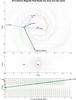 |
Fig. 1 Plots of the magnetic field from JF12. Top panel: top view of the X–Y plane of the Galaxy cut through Z = 0. The green arrows show the x–y coordinate system for SNR G296.5+10.0. The dashes on the x-axis are marked at 1 kpc intervals. The purple, dashed arrows show other longitudes, l = 55°, where the GMF is primarily along the line of sight and l = 170° and l = 355°, where the GMF is primarily perpendicular to the line of sight. The filled, red circle marks the Galactic center and the filled, green circle marks the position of the Sun. Center panel: X–Z plane cut through Y = 0. As in the top panel, the filled, red circle marks the Galactic center and the filled, green circle marks the position of the Sun. The shape of the X-field can be seen. Bottom panel: GMF lines are shown as cut along l = 296.5°. Here the horizontal axis of this plot is in the X–Y plane of the Galaxy along l = 296.5°. The vertical axis of this plot shows the z-axis of the Galaxy. As in the top panel, the green arrows show the primed coordinate system, in this case the x–z coordinates, for the case of SNR G296.5+10.0, which has b = 10.0°. The dashes on the x-axis are marked at 1 kpc intervals as in the top panel. Here, one can see that for d = 1 kpc, the GMF vectors are nearly pointed along the z-axis. |
The disk component is purely in the X–Y plane and includes a molecular ring between 3 kpc and 5 kpc (Galacto-centric radius) that is purely azimuthal with a constant field strength, bring = 0.1 μG. Beyond 5 kpc, there are eight logarithmic spiral regions at radii: 5.1, 6.3, 7.1, 8.3, 9.8, 11.4, 12.7, and 15.5 kpc (the radii where the spiral arm boundaries cross the negative X-axis). The disk field extent is symmetrical with respect to the mid-plane and transitions to the toroidal halo field at a height of ~0.40 kpc.
The toroidal component is a purely azimuthal halo component that is characterized by separate field amplitudes in the north (Bn = 1.4 μG, with a transition radius rn = 9.22 kpc) and south (Bs = −1.1 μG, with a transition radius rs> 16.7 kpc), and with a vertical scale height of ~5.3 kpc (see Eq. (6) of JF12).
The out-of-plane halo component is described by an X-shaped field, primarily motivated by radio observations of haloes in external edge-on galaxies (Beck 2009; Beck & Wielebinski 2013; Krause 2015). This component is axisymmetric and has a poloidal shape, lacking any azimuthal form since this is included in the toroidal field component. The X-field component takes the form: 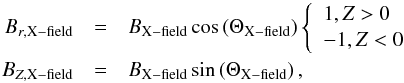 (1)where ΘX−field is the elevation angle, which is a function of radius and ΘX−field = 90° at r = 0 and ΘX−field = 49° at r = 4.8 kpc, and BX−field = 4.6 μG (field strength of the X-field component at the origin).
The total GMF is then the sum of the three components (as illustrated in Fig. 1):  (2)
(2)
3. Previous modeling of bilateral SNRs
It has been suggested that the observed morphology of bilateral SNRs is greatly influenced by the distribution of the CREs (e.g., Petruk et al. 2009; Bocchino et al. 2011; Reynoso et al. 2013). Two alternative distributions are often considered: the distributions for so-called quasi-parallel and quasi-perpendicular shocks (see Jokipii 1982; Leckband et al. 1989; Fulbright & Reynolds 1990 and references therein), which show distinct observed morphologies given the same magnetic field configuration. In particular, the axis of bilateral symmetry of the radio synchrotron emission is rotated by 90° between the two cases. In the quasi-perpendicular case, the shock-normal is perpendicular to the ambient field, but the axis of bilateral symmetry is aligned with the ambient field. In the quasi-parallel case the opposite is true; i.e., the shock-normal is parallel to the ambient field, while the axis of bilateral symmetry is perpendicular to the ambient field.
For the case of SN1006 in particular, the matter of which distribution is correct is still debated, with some arguing for the quasi-perpendicular scenario (e.g., Petruk et al. 2009; Schneiter et al. 2010) and others arguing for the quasi-parallel scenario (e.g., Rothenflug et al. 2004; Bocchino et al. 2011; Schneiter et al. 2015).
For the purposes of this study, we choose to use an isotropic distribution where the CREs are distributed uniformly in a shell. This will reveal the SNR morphology as if it were dependent solely on the compressed magnetic field. The overall shape of the morphology of the radio synchrotron emission in the quasi-perpendicular case, which despite it being more physically motivated than the isotropic case, is qualitatively the same as the isotropic case in a shell (see Fig. 2 and also Fulbright & Reynolds 1990 and references therein). Although quantitatively these two cases are different, the goal of this study is a qualitative analysis to show whether the morphology of SNRs obtained from the compressed GMF alone is consistent with the observed morphology in a large sample. We intend to investigate the difference between the quasi-parallel and quasi-perpendicular cases in a future study.
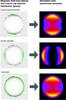 |
Fig. 2 Geometry of CRE distributions for quasi-perpendicular shocks (top), quasi-parallel shocks (middle), and the isotropic case (bottom) and the corresponding simulated synchrotron emission, which has been normalized for display purposes. This cartoon is intended to qualitatively show the distribution of the CREs with respect to the magnetic field geometry. It is not intended to be representative of the precise quantitative distributions. |
We account for complexities such as varying Galactic latitude, which will introduce a projected component that is perpendicular to the line of sight, and the effect of an intrinsic vertical GMF component. We find that these additions are very important for a global analysis of the morphology of axisymmetric SNRs.
We also investigate the global effects on SNRs in the context of the GMF at varying longitudes. Using a global sample of SNRs there is the suggestion of a correlation between the bilateral axis angle, ψ, and the orientation of the Galactic magnetic field. This relationship has the potential to reveal important information on the Galactic field as Kothes & Brown (2009) have previously suggested. For example, the presence of a reversal will imply an abrupt change in ψ. This is because the field model includes sign flips in the spiral component of the disk field, which alone would not change the morphology of the SNR, but when added to the smooth toroidal component, the total field orientation (not just the sign) changes. This in turn implies an abrupt change in ψ. This also gives a potentially new method to place constraints on distances to SNRs; in particular those at Galactic longitudes where the direction of the magnetic field, and thus the model SNR morphology, is changing rapidly along the line-of sight. SNRs could also be used to place constraints on distances to features, such as reversals, in the GMF.
4. Selection of the SNRs
For this paper we are studying the extent to which the SNR morphology and radio synchrotron emission are related to the regular component of the GMF that has been compressed by the SNR shock wave. Hence, we wish to include only the cleanest and most clearly-defined shells where the shell morphology is more likely not to be significantly altered through interaction with local enhancements in surrounding gas, turbulence in the GMF, nor influenced by a pulsar or a pulsar-wind nebula (PWN). In order to examine the appearance of the SNRs, we have searched the literature and data archives to collect the best-available radio images of all SNRs, excluding the pure shell-less PWNe; i.e., those that are classified as any type other than the filled-center type as defined by Ferrand & Safi-Harb (2012)2 and Green (2014). This is a total of 293 objects. We compile all radio images in a companion website, Supernova remnant Models and Images at Radio Frequencies (SMIRF)3. In Table 2 we summarize the numbers of SNRs of each type. This table represents the up-to-date numbers at the time of this writing; however the website is dynamic and classifications and exact counts of SNRs of various types are subject to change.
Thermal composite-type (also called mixed-morphology), plerionic composite-type, and unknown-type SNRs are considered, but with caution since these objects may involve more complex physics due to the presence of a central compact object and/or local enhancements of the ISM.
The thermal composite-type SNRs exhibit thermal X-ray emission in the SNR interior, but lack the shell seen at radio wavelengths. While the mechanisms responsible for their X-ray emission are still not fully understood, these remnants are generally found to be interacting with nearby dense interstellar structures, thus complicating our modeling and analysis. There are five thermal composites that have a very clearly defined axisymmetric morphology: G021.8–00.6, G116.9+00.2, G166.0+04.3, and G359.1–00.5, plus G093.3+06.9 that is also labeled as a plerionic composite (see Table 2 for a summary of the numbers of thermal composite SNRs of each type).
The plerionic composite-type may be influenced by the central compact object and surrounding nebula. These are included only in cases where we can be convinced that the shell is large compared to the PWN and the central pulsar is far enough away from the shell walls that we judge its influence to be negligible. Only one plerionic composite-type SNR is considered to be very clearly defined: G119.5+10.2 (plus G093.3+06.9 mentioned above).
We also looked at SNRs with unknown type. None of these are clearly defined, but four have possible, though poorly defined axisymmetric morphology. A notable one in this category is G039.7–02.0 (W50), which could possibly be an example of an axisymmetric type with jets from the binary source SS433.
There are 199 SNRs that are defined as shell-type (Ferrand & Safi-Harb 2012). Based on the images that we reviewed, the morphology of 112 are not consistent with what we call axisymmetric (i.e., a clear double- or single-sided shell), and we do not consider them further4. Some of these non-axisymmetric type SNRs have a completely undefined structure, while others have a defined, yet filamentary structure, which have significant emission through the center of the shell instead of just at the edges. Still others have a ring-like or round appearance (there are 15 out of 293 that we consider to have a very clearly defined or somewhat defined round appearance). These may prove to be interesting SNRs to analyze in future work (see Sect. 2), but we disregard them for the present analysis. This leaves 87 out of the 199 shell-type SNRs that we classify as axisymmetric.
In total, we have a sample of 112 SNRs with an axisymmetric (or possibly axisymmetric) morphology, including the selected thermal composite, plerionic composite, unknown, and shell-type objects (see Table 2). We assigned a level of uncertainty to the classification using the labels: very clearly defined (33 SNRs), somewhat defined (21 SNRs), and not clearly defined (58 SNRs)5. The analysis in this paper will only include the 33 SNRs with very clearly defined, clean morphology.
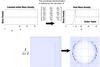 |
Fig. 3 Illustration of the technique used to determine the coordinate transformation matrix (Jacobian) and using it to transform the magnetic field vectors. The model uses the values from the NE2001 thermal electron density model (both local to the SNR and elsewhere along the line of sight). The technique assumes that the initial thermal electron mass density is constant locally around the SNR, which is approximately true for the NE2001 model. |
5. Description of our model
5.1. Outline of the modeling procedure
We use the Hammurabi code (Appendix B) to model the Stokes I, Stokes Q, and Stokes U synchrotron emission (defined below) at the coordinates of each of our selected SNRs for eleven discrete distances: 0.5, 1, 2, 3, 4, 5, 6, 7, 8, 9, and 10 kpc. The SNR is modeled as a spherical shock or bubble, which deforms the field lines of the JF12 GMF model at the SNR location (see Sect. 5.2). Since the Galactic field model varies with distance, the model SNRs show differences in morphology as a function of distance as well. This potentially provides a constraint on the distance of an SNR based on its morphology. For each SNR position and distance, the modeling process is as follows:
-
1.
Run Hammurabi to output the JF12 model of the GMF and theNE2001 thermal electron density for the direction of an SNR on aparticular line of sight (i.e., for a particular set of Galactic coordi-nates). The field is written with a resolution of 1 pc per voxel. Thetotal size of the volume is determined by the assumed radius of themodel SNR and the distance. Table 1 summarizesthe physical and angular sizes for the SNRs bubbles modeled atthe various distances. These sizes were chosen to be consistentwith the approximate average size expected for an SNR in theSedov phase. At nearer distances, a smaller size is chosen to re-duce computation time (reduces the overall size of the volume)and reduce the angular size to something that is consistent withthe observations (the SNR with the largest angular scale in oursample is G315.1+02.7, which has a size of 190′). Note that the integration that computes the total Stokes I, Stokes Q, and Stokes U parameters is not done at this stage. Rather, Hammurabi is used at this stage only to write the magnetic field components and thermal electron density at each point along a particular line of sight to a file.
-
2.
Using Matlab, read the portion of the magnetic field and thermal electron density data files (output from Hammurabi) at the position of the SNR and apply the numerically defined coordinate transformation function (see Sect. 5.2) to these voxels. These sections of the files are then overwritten with the newly calculated transformed magnetic field and thermal electron density values.
-
3.
Run Hammurabi a second time. This time the magnetic field and thermal electron density data files are passed as input to Hammurabi. In addition, an analytical model of the distribution of CRE is defined within the code. The ambient CRE density is defined as in Appendix B while the CRE within the shell of the SNR is compressed uniformly around the shell as the thermal electrons. Hammurabi then numerically integrates and produces output for the model Stokes I,Q, and U parameters, which is also described in Appendix B.
5.2. Supernova remnant model
After the initial supernova explosion, the conventional description is that the SNR is ejecta-dominated until the swept-up mass exceeds the mass of the ejecta. It is at this point, roughly 1000 years after the explosion (depending on the progenitor, explosion energy, and ambient density), that the blast wave can be described using a Sedov-Taylor solution (Sedov 1959; Korobeinikov 1991). This solution has the advantage of being self-similar with a well-defined analytical form that describes the thermal electron mass density as a function of radius (see Fig. 3). We model the thermal electron density and magnetic field of a spherical shell compressed by a Sedov-Taylor blast wave. We note that some SNRs in our sample are either quite young (e.g., G001.9+00.3) or possibly in a radiative phase of expansion (e.g., the thermal composites), and as a result, are likely not in the Sedov-Taylor phase. We argue however that the ambient medium is still compressed enough that their morphology can be approximated by using the Sedov-Taylor density model. Furthermore, we are here mostly concerned with their overall morphology at radio wavelengths, rather than an absolute measurement of their emission in radio or other wavelengths.
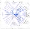 |
Fig. 4 Position of the 33 SNRs in our sample showed plotted on the Galaxy with field vectors from JF12 drawn for z = 0, b = 0. The Sun’s position shown is at −8.5 kpc from the Galactic center. The thin lines represent the distance estimate from the literature while the thicker, lighter colored lines represent the best fit distance from the models. |
In order to compute the magnetic field in the shell, we assume that the magnetic field vectors are frozen-in to the ambient plasma, which is a common assumption for ionized plasma. We then adopt the method of Franzmann (2014), who developed a coordinate transformation technique to model the magnetic field in molecular cloud cores.
The transformation, outlined in Appendix C, takes an initial 3D magnetic field, B, which is compressed by a spherical shock that drags the field lines and gives the appropriately transformed magnetic field, B′. While the initial thermal electron mass density is assumed to be constant in the region surrounding the SNR, the initial magnetic field is not required to be uniform (as illustrated in the example shown in Fig. 3); it can have an arbitrary distribution. The SNR can thus be modeled in the context of the Galaxy by using this method to transform the model GMF and insert an SNR at a particular location.
The process of using this coordinate transformation to alter the magnetic field results in an output that is compressed at the edges, and we measure the magnitude of the compressed field to be around six times greater that the initial field (see Fig. 3). An amplification factor of six agrees with that derived by van der Laan (1962) for the case of spherical geometry (see their Eq. (57)). The magnetic field is not compressed at locations where the shock normal is oriented parallel to the magnetic field as illustrated in Fig. 3. Recent X-ray observations show that the magnetic field is amplified by a much larger factor than this, which is most likely due to local turbulent acceleration that amplifies the already compressed field (e.g., Uchiyama et al. 2007; Uchiyama & Aharonian 2008; Reynolds et al. 2012). We do not take this additional amplification into account, but note that this would impact the quantitative result, and not the qualitative morphology that is the focus of this work.
6. Comparison of the models to data
We present results of modeling 33 SNRs distributed around the Galaxy (see Fig. 4 and Appendix D). In order to compare the data to the model we use two parameters. The first parameter is the angle ψ, which we remind the reader is the projected angle between the axis of bilateral symmetry and the Galactic plane. The second parameter is the ratio of the peak brightness level between the two sides. For the models, the angle, ψ was found by measuring the mean value of the pixels along a line extending across the diameter of the model SNR. The line was rotated in 1° increments and the position where the mean of the pixels along the line has a minimum value was taken as the angle through the symmetry axis. The real data images are not as clean as the model images as they contain background emission, point sources, and noise. Thus we did not obtain good results measuring the angle ψ on the real data using this method and it was found that a by-eye method resulted in a better measurement. Therefore we measured ψ by using a rectangular box sized to fit the gap between the lobes. We rotated the box in 1° increments and the best angle was determined based on how well it apparently divides the emission into two distinct lobes. We estimate the uncertainty of this measurement to be ±5°. This estimate is based on the variation resulting from repeated independent measurements.
After the angle is determined, a circular region with 8 pie-slice shape wedges is defined, centered on the SNR (this procedure was done for both the models and the data). Two of the slices are centered on the symmetry axis, which means two other slices should be centered on the bilateral lobes. We then found the ratio of the mean brightness in the two wedges for the SNR lobes on opposite sides (i.e., mean north limb divided by mean south limb). This ratio was measured for all of the models using the automatically determined best-fit angle and for the data using the by-eye best-fit angle in each case.
If the SNR were perfectly symmetrically bilateral the ratio should be 1. If this ratio is >1 it means the SNR/model is brighter in the north, and if this ratio is <1 it means it is brighter in the south. We determined the best-fit model overall by looking first at the best fitting angles and then comparing the ratios. If two models had an angle with an equally good fit, then the ratio was used to select the best model overall. These results are summarized in Table 3.
Summary of the results for the data with the corresponding best fit model.
6.1. Features of the models
As shown in Appendix D, most of the models have a symmetric, bilateral appearance with two well separated limbs of uniform brightness. This is because the magnetic field is relatively uniform at the particular location where the SNR was modeled and thus the compressed field is more or less equal on both sides. However some of the models have a circular morphology or other unusual features.
In some cases, the models have a round or circular appearance, for example, the case of G036.6+02.6 at d = 5 kpc (see Appendix D). This is due to the magnetic field being primarily directed along the line of sight at those locations (i.e., the vectors are coming directly at the observer or pointing directly away from the observer). It should be noted that these round models should be intrinsically fainter since the observed synchrotron emission depends on the perpendicular component of the magnetic field. This brightness difference is not apparent in the figures since the model images have been normalized for the purpose of comparing them to the observed SNR morphology.
In other locations, we find that the model SNRs have one limb significantly brighter than the other; for example, G028.6–00.1 at distances of 2–4 kpc (see Appendix D). This brightness difference can be explained by asymmetries in the magnetic field model. In some cases, if the field is changing, there can be a difference between the two limbs where the field has a larger line-of-sight component on one side and a larger perpendicular component on the other. In this case the limb with the stronger perpendicular component will be brighter. In other cases, the magnitude of the field is stronger on one side compared to the other, which will also result in an asymmetry in the brightness.
For some models, some sharp and dark features appear in the images. For example, for the case of G317.3–00.2, the model images up to 6 kpc show such a feature. These apparent lines are the result of sharp transitions in the magnetic field model and can be emphasized by the vector addition of the various components of the model (see Sect. 2.2.1). These transitions will appear sharper and somewhat unphysical in these models. It is possible that such transitions are present in the real Galactic field although they would likely be smoother and less abrupt.
In Fig. 5 we show several models at the position of G317.3–00.2 at a distance of 2 kpc to show the impact of excluding the various field components. In this example, the X shape is contributing a line-of-sight component, in addition to a vertical GMF component. Thus, the model that includes the X-field shows strong asymmetry with the southern limb of the SNR being much brighter, which is consistent with the data. Figure 5 shows that for this particular example, the asymmetry is due primarily to the inclusion of the X-field and illustrates the impact of including this component.
 |
Fig. 5 Top: models at the position of G317.3–00.2 and for a distance of 2 kpc showing the impact of excluding the various magnetic field components. Bottom: corresponding magnetic field vectors shown in the z–y plane (i.e., the plane of the sky, see Appendix A) and cut through the center of the SNR bubble. Left panel: only the disk field, Bdisk has been included. The two limbs are more or less uniform in brightness (slightly brighter in the north). Center panel: toroidal halo field, Btor has been included. There is now some asymmetry introduced since the magnetic field is stronger in the south with the addition of the toroidal halo component. Right panel: the X-field, BX−field, has now been included. The vector sum of these components has now made the field in the northern half of this SNR much smaller in magnitude and the direction has changed (there is now a much stronger line-of-sight (x) component in the northern half, though that is not visible on this figure). Thus the model SNR shows a high degree of asymmetry, which strongly resembles the data. |
7. Results and discussion
We find that 25 out of the 33 SNRs have an angle that agrees with the angle from the Galactic model within 10° (see Fig. 6). When we compare the brightness, we find that for 23 out of 33 SNRs the models and data agree in the sense that they are brighter/fainter on the same side (i.e., both would be bright in the north or both bright in the south). In five of the cases the brightness difference is border-line where both the model and data have values close to one (i.e., equally bright on both sides). There are five cases (G021.8–0.6, G046.8–00.3, G054.4–00.3, G166.0+04.3, G327.4+1.0) where there is a significant disagreement between the brightness distribution between the model and the data in terms of this measurement. It is important to note that at least two of these cases (G021.8–0.6 and G166.0+04.3) are known to be thermal composites interacting with a molecular cloud.
The fact that nearly 75% of our clean sample of axisymmetric SNRs is well modeled with the JF12 model provides strong support for the impact of the GMF on SNR morphology, as well as the need for a vertical component for Galactic field models (see also Sect. 7.2). We remind the reader that we had purposely selected the clean sample in our investigation in order to minimize observational bias based on poor-quality data.
We did a preliminary review of the other 113 SNRs in the axisymmetric sample (see Sect. 4) to compare the models and data based on a visual inspection. Even though in many cases it is difficult to judge the fit due to poor quality data, we find that there are intriguing matches for a number of SNRs between model and data that are good prospective case studies. The models for all 113 SNRs can be reviewed on the companion website (SMIRF6).
Nearly 25% of our sample is clearly not well fitted by the Galactic field model, implying that other effects are in play. Aside from local electron acceleration effects (e.g. associated with quasi-parallel/perpendicular mechanisms) and turbulence that are not accounted for in this work, additional factors in affecting the SNR morphology include the SN progenitor and expansion into the CSM. This is particularly expected for the youngest SNRs that are still under the influence of the progenitor’s mass-loss history (e.g., Chevalier 1982). Significant departures from the standard Sedov-Taylor evolutionary phase can also arise from the SNR expansion into stellar wind bubbles blown by the pre-supernova progenitor. In fact, it has been argued that SNRs resulting from explosions of very massive stars can spend a significant fraction of their lifetime in their progenitor bubbles, which would then affect their evolution and morphology for tens of thousands of years (see e.g., Dwarkadas 2005, 2011). Therefore, they interact with the ISM at a much later stage in comparison to the type Ia remnants expanding normally in a less complex CSM. A systematic study of the SNR sample taking into account known age and classification (Ia vs. core-collapse) will help us address this question. It is also possible that in some cases the progenitor bubble itself is carved by the GMF. Interesting case studies include G296.5+10.0 whose striking bilateral morphology has been suggested to be affected by a magnetized progenitor wind (Harvey-Smith et al. 2010). Overall, we can successfully model the morphology of an impressively large number of axisymmetric SNRs and while these other effects can have a significant bearing on the appearance of an SNR, the GMF still seems to be the dominant factor.
7.1. Distance constraints
Depending on the longitude of the SNR, the orientation (pitch angle) of the GMF model, and how the model varies along the line of sight for that direction, the models can fairly tightly constrain the distance in some cases (for example G003.7–00.2, G093.3+06.9, G296.5+10.0, G327.6+14.6, and G350.0–02.0); while in other cases, a much larger range of distances could account for the observed emission. We remind the reader that there are significant uncertainties in the specific features of the JF12 model (see Sect. 2.2). Thus one must be cautious with interpreting these results for individual SNRs and dedicated case studies are necessary for constraining the distance uncertainties in specific instances. This is particularly true for SNRs near the Galactic center where the GMF is more uncertain and may be dominated by turbulent magnetic fields.
Our best fit distances are determined by comparing the angles and brightness ratios of the data with the model. These are summarized in Table 3. Local variations in the magnetic field could change the distance interpretation but we expect that the large-scale field would dominate in most cases, particularly in these cases where the shell is clear and well-defined.
When we compared the distances for the best fit of the model with the distances given in the literature (and compiled in SNRcat, Ferrand & Safi-Harb 2012) we find that out of the 33 SNRs, 18 have some distance estimate published in the literature and our results agree with 15 of the 18 distance estimates. These results are summarized in Table 3 (see also Fig. 4). Only 3 SNRs have quite poor agreement: G065.1+0.6, G332.0+0.2 and G359.1–00.5.
G065.1+0.6: the distance to the shell is estimated to be 9–9.6 kpc (Tian & Leahy 2006) whereas our best-fit model gives  kpc. We do note that the distance to a nearby pulsar (PSR J1957+2831), possibly associated with the shell, is estimated to be 7 kpc, which is in agreement with the upper limit of our range. A further investigation of the distance to this remnant and its association with the pulsar is needed.
G332.0+0.2: this SNR is estimated to be at >6.6 kpc (Caswell & Haynes 1975), which is a kinematic distance based on measurements of OH absorption. This disagrees with our best-fit model distance of  kpc. Given that the size of the radio shell is 12′, at a distance of 1 kpc, the shell’s physical size would be 3.4 pc, which would imply that the object is quite young. Further investigation and a new distance estimate are required.
G359.1–00.5: the Suzaku X-ray study of this object (Ohnishi et al. 2011) implies a distance close to the Galactic center and the authors assume a distance of 8.5 kpc, which is in agreement with other work that puts the distance at 8–10.5 kpc (Frail 2011; Uchida et al. 1992). Our best fit model puts the distance at  kpc, but we note that the JF12 model does not attempt to model the GMF right at the Galactic center (see also Fig. D.1 showing that there are no model fits for distances between 7 and 10 kpc, which bracket the distance from observations).
The fact that the distance agrees in the majority of cases supports the use of this model as a distance indicator in cases where the distance to the SNR is unknown. Conversely, quality imaging of SNRs, combined with good distance information, can give valuable input to determination of distances to features of the GMF.
7.2. Comparison with Sun et al. (2008)
In addition to JF12, we computed models for all axisymmetric SNRs using the GMF model of Sun et al. (2008), which does not include a Z-component. These two GMF models were both derived from fits to observations and the models both use the same spiral pitch angle. Since the field strength does not come into this analysis, the main difference between the two models is the geometry, namely the distances and directions of the reversals and the addition of the X-field in JF12. For each model we selected the distance that matches best, but in many cases, no good match was available, especially for the models using Sun et al. (2008). Figure 6 illustrates that the JF12 model provides a substantially better fit to the data, particularly in terms of ψ, in nearly all cases.
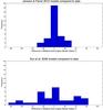 |
Fig. 6 Histogram of the differences, ψmodel−ψdata, for the best fitting models of JF12 (top) and Sun et al. (2008) (bottom). In the case of JF12, out of 33 SNRs, 25 have a difference that is < 10°, which are in agreement within our uncertainty. In the case of Sun et al. (2008), only 10 SNRs have a difference that is < 10°. |
In our sample of 33 SNRs, there are about nine cases where the Sun et al. (2008) model gives a reasonably good fit. In most cases this occurs where the orientation of the symmetry axis of the SNR is parallel to the Galactic plane and where the Galactic latitude is small (< | 2° |). Figure 7 shows a comparison of the two field models for three illustrative SNRs: one at relatively high latitude, G296.5+10.0; one at a mid-range latitude, G016.2–02.7; and one in the Galactic plane, G046.8–00.3.
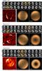 |
Fig. 7 Comparison of SNR models for three example SNRs: G296.5+10.0 (high-latitude), G016.2-2.7 (mid-latitude), and G046.8-0.3 (in the plane). All models from 0.5 to 10 kpc are shown (as described in Fig. D.1) for both GMF models: the Sun et al. (2008) (Sun08) and JF12. The orange box highlights the best fit in each case. Below the model strips we show the data (left) as well as the corresponding best fit model for JF12 (center) and Sun08 (right) . The model polarization magnetic field vectors are overlaid in green. |
7.3. Magnetic fields of the SNRs
The model observations give us simulated Stokes Q and U polarization parameters. These are used to produce polarized intensity ( ) and polarization angle (
 ) values that are used to make plots of the simulated magnetic field as in Fig. 7 (where the PA gives the orientation of the electric field).
Of the 33 SNRs in our very well defined sample, 13 have a magnetic field that has been observed through polarization studies. Of these, 9 have been observed to have a tangential magnetic field: G016.2–02.7, G065.1+00.6, G093.3+06.9, G119.5+10.2, G127.1+00.5, G156.2+05.7, G166.0+04.3, G182.4+04.3, and G296.5+10.0. In every one of these cases, simulated magnetic field plots for the models also show a tangential magnetic field. Two such cases, G016.2–2.7 and G296.5+10.0, are shown in Fig. 7.
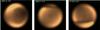 |
Fig. 8 Simulated polarization vectors for SNRs where observations show that they have mixed magnetic fields. These are all shown for a distance of 4 kpc, which is the best-fit distance for G054.4–0.3 and G116.9+0.2. In the case of G021.8–0.6, the best fit distance is at 5 kpc. The magnetic field at that distance is tangential, but at 4 kpc, which is still a reasonable fit, the field shows more characteristics of being mixed. |
Roger et al. (1988) suggest that a vertically oriented field may be responsible for the appearance of SNRs G296.5+10.0 and G327.6+14.6 (SN1006) and our study supports this conclusion. We note that RM observations by Harvey-Smith et al. (2010) lead those authors to conclude that G296.5+10.0 has a radial field, possibly due to the progenitor star. However the observations have very poor UV coverage and are only sensitive to smaller structures making this conclusion uncertain. Additionally, RM observations are sensitive only to the line-of-sight component of the magnetic field. We propose that a twisted vertical field could explain both the RM result and still be consistent with a vertically oriented tangential field as shown by Milne (1987).
Three SNRs in our sample have what we term mixed magnetic fields, where the field is not obviously tangential or radial. These are G021.8–00.6, G054.4–00.3 and G116.9+00.2. Both G021.8–00.6 and G116.9+00.2 are thermal composite-type SNRs. In addition, two of these SNRs G021.8–00.6 and G054.4–00.3 were noted above as having poor fits in terms of the brightness ratio, which is perhaps not surprising since they seem to be more complex cases. G054.4–00.3 in particular is interesting in that the morphology of the model bears a striking similarity to the data despite the fact that the brightness ratios do not agree. The simulated polarization vector plots for these SNRs (Fig. 8) also show deviations from a purely tangential field and thus would also be considered to have mixed magnetic fields.
Only two SNRs in our sample have been observed to have radial fields: G046.8–00.3 and G327.6+14.6 (SN1006). It is interesting that in the case of G046.8–00.3, the simulated polarization vector plot for the JF12 is tangential, but the plot using the Sun et al. (2008) model at the corresponding distance (4 kpc) does indeed show a radial magnetic field (see Fig. 7).
G327.6+14.6 (SN1006) has also been observed to have a radial field (Reynoso et al. 2013), but the observations also reveal the suggestion of a tangential field at the edges. In our model, the simulated polarization vector plot for the JF12 field is tangential, but we note that the field configuration at this location is close to being directed primarily along the line of sight, which would produce a radial field. This will be addressed in a future dedicated study.
8. Conclusions and future work
We have focused in this paper on the cleanest and most complete sample of Galactic axisymmetric SNRs, i.e., those showing an axis of symmetry often referred to in the literature as bilateral or barrel-shaped SNRs. We have modeled these remnants using the comprehensive GMF model of Jansson and Farrar (2012a, JF12), which takes into account for the first time an off-plane, X-shaped component of the GMF that is motivated by observations of the magnetic field in external galaxies7. We stress it is not the details of the JF12 model that matter the most for our modeling, but rather the presence of the vertical, X-shaped component (described in detail in Sect. 2.2) that is not included in previous models. We have demonstrated that:
-
1.
We can reproduce the observed morphologies of individualSNRs, in particular the bilateral axis angle, through a simple andphysically motivated model of an SNR expanding into theambient GMF. In addition to the morphology, the magnetic fieldspredicted by the models (i.e., tangential or radial) are consistentwith the observed magnetic fields in nearly all cases.
-
2.
If the large scale Galactic field is known, this method can predict distances to SNRs, or conversely, if SNR distances are known, they could constrain the large-scale GMF at their position.
-
3.
A systematic comparison of a sample of SNRs at different positions in the Galaxy in combination with this modeling method can distinguish between two large-scale GMF models, even given the uncertainties in the distances.
-
4.
A large-scale GMF model without a vertical component is not consistent with our sample of SNRs. Therefore, either the large-scale Galactic field must have a vertical field component, or the simple and physically motivated model of SNR expansion into the ambient field is missing an element that must not only alter the morphologies of individual SNRs (e.g., ambient density changes) but must do so in a systematic way throughout the Galaxy. It is difficult to envision such a mechanism that is as simple and natural (and motivated by observations of external galaxies) as an X-shaped field component. Although it is suggestive, these results do not conclusively prove that the vertical field must have an X-shape. Nevertheless, this paper strongly supports the presence of a vertical halo component in the Milky Way Galaxy.
In future work, we plan to present a more detailed analysis of some select SNRs with sufficient data in the radio (and in X-rays for the non-thermal shells), comparing our results not only to the SNR morphology, but also to the observed radio polarization and rotation measure observations where possible. Furthermore, SNRs with a ring-like or round appearance are also an interesting area for future study with this modeling to investigate whether some of them may be a result of line-of-sight magnetic fields.
The model used in this study (JF12) included only the regular component of the GMF, and did not include any turbulent component that would be associated with the large-scale Galactic field or local-to-the-SNR acceleration mechanisms. In a future study we would like to investigate the impact of turbulence on SNR morphology. Since the sample of Galactic SNRs represents a range of different ages and thus different scales, SNRs can be used as a tool to investigate the scale of the turbulence. In particular, an SNR that is much smaller than the scale of the GMF turbulence may see the turbulent component as a regular component. In that case the SNR may still show axisymmetric morphology, but at an angle consistent with the turbulent magnetic field (Gwenael Giacinti, priv. comm.). Thus a careful analysis of SNRs at various scales may give some important clues to the outer scale of the turbulence spectrum in the GMF.
Other possible extensions of this work include investigating global properties of the GMF such as the pitch angle of the spiral pattern and the precise shape of the vertical field. Another exciting future extension is to conduct an analysis of SNRs with well-constrained distances from other robust methods, to estimate distances to features in the GMF such as reversals and transitions.
G327.6+14.6, has the highest latitude and is thought to be relatively nearby at a distance of 1.6–2.2 kpc (Ferrand & Safi-Harb 2012) and thus a height of about 400-550 pc above the plane, or very close to the disk-halo boundary.
These are labeled as “Not axisymmetric” in Table 2.
All 112 SNRs have been modeled and those models are available on the companion website (SMIRF: http://www.physics.umanitoba.ca/snr/smirf/).
We have made all of these images and models available on our companion website (SMIRF: www.physics.umanitoba.ca/snr/smirf/).
Acknowledgments
This research was primarily supported by the Natural Sciences and Engineering Research Council of Canada (NSERC) through a Canada Graduate Scholarship (J. West) and the Canada Research Chairs and Discovery Grants Programs (S. Safi-Harb). The modeling was performed on a local computing cluster funded by the Canada Foundation for Innovation (CFI) and the Manitoba Research and Innovation Fund (MRIF). We acknowledge and thank Gilles Ferrand for useful discussions and contributions to SNRcat used in this study, and Erica Franzmann for her assistance with the coordinate transformation code. The radio images presented in this paper and companion website made use of data obtained with the following facilities: CHIPASS 1.4 GHz radio continuum map, Canadian Galactic Plane Survey (CGPS) and other data from the Dominion Radio Astrophysical Observatory, Southern Galactic Plane Survey, Effelsberg 100 m Telescope and Stockert Galactic plane survey (2720 MHz) (via MPIfR’s Survey Sampler), Molonglo Observatory Synthesis Telescope (MOST) Supernova Remnant Catalogue (843 MHz), Sino-German 6 cm survey. Additionally we acknowledge the use of NASA’s SkyView facility (http://skyview.gsfc.nasa.gov) located at NASA Goddard Space Flight Center for the data from the 4850 MHz Survey/GB6 Survey, NRAO VLA Sky Survey, Sydney University Molonglo Sky Survey (843 MHz), and the Westerbork Northern Sky Survey (325 MHz Continuum). Very Large Array (VLA) data was acquired via the NRAO Science Data Archive and the Multi-Array Galactic Plane Imaging Survey. We thank Michael Bietenholz and David Kaplan for providing the VLA images of G021.6–00.8 and G042.8+00.6, respectively. This research made use of APLpy, an open-source plotting package for Python (http://aplpy.github.com) and Astropy, a community-developed core Python package for Astronomy (Astropy Collaboration, 2013). This research also made use of Montage. It is funded by the National Science Foundation under Grant Number ACI-1440620, and was previously funded by the National Aeronautics and Space Administration’s Earth Science Technology Office, Computation Technologies Project, under Cooperative Agreement Number NCC5-626 between NASA and the California Institute of Technology. This research has made use of the NASA Astrophysics Data System (ADS). We are grateful to and thank the referee for the helpful and thorough comments that significantly improved the paper.
References
- Beck, R. 2009, Ap&SS, 320, 77 [NASA ADS] [CrossRef] [Google Scholar]
- Beck, R., & Wielebinski, R. 2013, in Magnetic Fields in Galaxies (The Netherlands, Dordrecht: Springer), 641 [Google Scholar]
- Boas, M. L. 2005, Mathematical Methods in the Physical Sciences (Wiley) [Google Scholar]
- Bocchino, F., Orlando, S., Miceli, M., & Petruk, O. 2011, A&A, 531, A129 [NASA ADS] [CrossRef] [EDP Sciences] [Google Scholar]
- Brown, J. C. 2002, Ph.D. Thesis. University of Calgary (Canada), Source DAI-B 63/08, 3755, Feb. 2003, 159 [Google Scholar]
- Brown, J. C., & Taylor, A. R. 2001, ApJ, 563, L31 [NASA ADS] [CrossRef] [Google Scholar]
- Caswell, J. L., & Haynes, R. F. 1975, MNRAS, 173, 649 [NASA ADS] [CrossRef] [Google Scholar]
- Chevalier, R. A. 1982, ApJ, 259, L85 [NASA ADS] [CrossRef] [Google Scholar]
- Condon, J. J., Griffith, M. R., & Wright, A. E. 1993, AJ, 106, 1095 [NASA ADS] [CrossRef] [Google Scholar]
- Condon, J. J., Cotton, W. D., Greisen, E. W., et al. 1998, AJ, 115, 1693 [NASA ADS] [CrossRef] [Google Scholar]
- Cordes, J. M., & Lazio, T. J. W. 2002, arXiv e-prints [arXiv:astro-ph/0207156] [Google Scholar]
- Dwarkadas, V. V. 2005, ApJ, 630, 892 [NASA ADS] [CrossRef] [Google Scholar]
- Dwarkadas, V. V. 2011, Mem. Soc. Astron. It., 82, 781 [NASA ADS] [Google Scholar]
- Ferrand, G., & Safi-Harb, S. 2012, Adv. Space Res., 49, 1313 [NASA ADS] [CrossRef] [Google Scholar]
- Frail, D. A. 2011, Mem. Soc. Astron. Ita., 82, 703 [Google Scholar]
- Franzmann, E. 2014, MSc Thesis, University of Manitoba (Canada), 227 [Google Scholar]
- Fulbright, M. S., & Reynolds, S. P. 1990, ApJ, 357, 591 [NASA ADS] [CrossRef] [Google Scholar]
- Gaensler, B. M. 1998, ApJ, 493, 1 [Google Scholar]
- Gorski, K. M., Hivon, E., Banday, A. J., et al. 2005, ApJ, 622, 759 [NASA ADS] [CrossRef] [Google Scholar]
- Green, D. A. 2014, Bull. Astron. Soc. India, 42, 47 [NASA ADS] [Google Scholar]
- Harvey-Smith, L., Gaensler, B. M., Kothes, R., et al. 2010, ApJ, 712, 1157 [NASA ADS] [CrossRef] [Google Scholar]
- Haverkorn, M. 2015, in Astrophys. Space Sci. Lib. 407, eds. A. Lazarian, E. M. de Gouveia Dal Pino, & C. Melioli, 483 [Google Scholar]
- Helfand, D. J., Becker, R. H., White, R. L., Fallon, A., & Tuttle, S. 2006, AJ, 131, 2525 [NASA ADS] [CrossRef] [Google Scholar]
- Inoue, T., Shimoda, J., Ohira, Y., & Yamazaki, R. 2013, ApJ, 772, L20 [NASA ADS] [CrossRef] [Google Scholar]
- Jaffe, T. R., Leahy, J. P., Banday, A. J., et al. 2010, MNRAS, 401, 1013 [NASA ADS] [CrossRef] [Google Scholar]
- Jansson, R., & Farrar, G. R. 2012a, ApJ, 757, 14 [NASA ADS] [CrossRef] [Google Scholar]
- Jansson, R., & Farrar, G. R. 2012b, ApJ, 761, L11 [NASA ADS] [CrossRef] [Google Scholar]
- Jokipii, J. R. 1982, ApJ, 255, 716 [NASA ADS] [CrossRef] [Google Scholar]
- Kesteven, M. J., & Caswell, J. L. 1987, A&A, 183, 118 [NASA ADS] [Google Scholar]
- Korobeinikov, V. P. 1991, Problems of Point Blast Theory (Springer Science and Business Media) [Google Scholar]
- Kothes, R., & Brown, J.-A. 2009, in IAU Symp. 259, eds. K. G. Strassmeier, A. G. Kosovichev, & J. E. Beckman, 75 [Google Scholar]
- Kothes, R., & Reich, W. 2001, A&A, 372, 627 [NASA ADS] [CrossRef] [EDP Sciences] [Google Scholar]
- Krause, M. 2015, Interstellar Gas Dynamics, 10, 399 [Google Scholar]
- Landecker, T. L., Routledge, D., Reynolds, S. P., et al. 1999, ApJ, 527, 866 [NASA ADS] [CrossRef] [Google Scholar]
- Leckband, J. A., Spangler, S. R., & Cairns, I. H. 1989, ApJ, 338, 963 [NASA ADS] [CrossRef] [Google Scholar]
- Manchester, R. N. 1987, A&A, 171, 205 [NASA ADS] [Google Scholar]
- Milne, D. K. 1987, Austral. J. Phys., 40, 771 [Google Scholar]
- Ohnishi, T., Koyama, K., Tsuru, T. G., et al. 2011, PASJ, 63, 527 [NASA ADS] [Google Scholar]
- Ohno, H., & Shibata, S. 1993, MNRAS, 262, 953 [NASA ADS] [Google Scholar]
- Orlando, S., Bocchino, F., Reale, F., Peres, G., & Petruk, O. 2007, A&A, 470, 927 [NASA ADS] [CrossRef] [EDP Sciences] [Google Scholar]
- Page, L., Hinshaw, G., Komatsu, E., et al. 2007, ApJSS, 170, 335 [NASA ADS] [CrossRef] [Google Scholar]
- Petruk, O., Dubner, G. M., Castelletti, G., et al. 2009, MNRAS, 393, 1034 [NASA ADS] [CrossRef] [Google Scholar]
- Pshirkov, M. S., Tinyakov, P. G., Kronberg, P. P., & Newton-McGee, K. J. 2011, ApJ, 738, 192 [NASA ADS] [CrossRef] [Google Scholar]
- Rand, R. J., & Kulkarni, S. R. 1989, ApJ, 343, 760 [NASA ADS] [CrossRef] [Google Scholar]
- Rengelink, R. B., Tang, Y., de Bruyn, A. G., et al. 1997, A&ASS, 124, 259 [NASA ADS] [CrossRef] [EDP Sciences] [Google Scholar]
- Reynolds, S. P., Borkowski, K. J., Green, D. A., et al. 2008, ApJ, 680, L41 [NASA ADS] [CrossRef] [Google Scholar]
- Reynolds, S. P., Gaensler, B. M., & Bocchino, F. 2012, Space Sci. Rev., 166, 231 [NASA ADS] [CrossRef] [Google Scholar]
- Reynoso, E. M., Hughes, J. P., & Moffett, D. A. 2013, AJ, 145, 104 [NASA ADS] [CrossRef] [Google Scholar]
- Roger, R. S., Milne, D. K., Kesteven, M. J., Wellington, K. J., & Haynes, R. F. 1988, ApJ, 332, 940 [NASA ADS] [CrossRef] [Google Scholar]
- Rothenflug, R., Ballet, J., Dubner, G. M., et al. 2004, A&A, 425, 121 [NASA ADS] [CrossRef] [EDP Sciences] [Google Scholar]
- Rybicki, G. B., & Lightman, A. P. 1979, (New York: Wilo-Interscience) [Google Scholar]
- Schneiter, E. M., Velázquez, P. F., Reynoso, E. M., & De Colle, F. 2010, MNRAS, 408, 430 [NASA ADS] [CrossRef] [Google Scholar]
- Schneiter, E. M., Velazquez, P. F., Reynoso, E. M., Esquivel, A., & De Colle, F. 2015, MNRAS, 449, 88 [NASA ADS] [CrossRef] [Google Scholar]
- Sedov, L. I. 1959, Similarity and Dimensional Methods in Mechanics (New York: Academic Press) [Google Scholar]
- Shaver, P. A. 1982, A&A, 105, 306 [NASA ADS] [Google Scholar]
- Sun, X. H., & Reich, W. 2009, A&A, 507, 1087 [NASA ADS] [CrossRef] [EDP Sciences] [Google Scholar]
- Sun, X.-H., & Reich, W. 2010, RA&A, 10, 1287 [Google Scholar]
- Sun, X. H., Reich, W., Waelkens, A., & Enßlin, T. A. 2008, A&A, 477, 573 [NASA ADS] [CrossRef] [EDP Sciences] [Google Scholar]
- Sun, X. H., Landecker, T. L., Gaensler, B. M., et al. 2015, ApJ, 811, 40 [NASA ADS] [CrossRef] [Google Scholar]
- Taylor, A. R., Gibson, S. J., Peracaula, M., et al. 2003, AJ, 125, 3145 [NASA ADS] [CrossRef] [Google Scholar]
- Tian, W. W., & Leahy, D. A. 2006, A&A, 455, 1053 [NASA ADS] [CrossRef] [EDP Sciences] [Google Scholar]
- Uchida, K., Morris, M., & Yusef-Zadeh, F. 1992, AJ, 104, 1533 [NASA ADS] [CrossRef] [Google Scholar]
- Uchiyama, Y., & Aharonian, F. A. 2008, ApJ, 677, L105 [NASA ADS] [CrossRef] [Google Scholar]
- Uchiyama, Y., Aharonian, F. A., Tanaka, T., Takahashi, T., & Maeda, Y. 2007, Nature, 449, 576 [NASA ADS] [CrossRef] [PubMed] [Google Scholar]
- van der Laan, H. 1962, MNRAS, 124, 125 [NASA ADS] [Google Scholar]
- Van Eck, C. L., Brown, J. C., Stil, J. M., et al. 2011, ApJ, 728, 97 [NASA ADS] [CrossRef] [Google Scholar]
- Waelkens, A., Jaffe, T., Reinecke, M., Kitaura, F. S., & Enßlin, T. A. 2009, A&A, 495, 697 [NASA ADS] [CrossRef] [EDP Sciences] [Google Scholar]
- Whiteoak, J. B., & Gardner, F. F. 1968, ApJ, 154, 807 [NASA ADS] [CrossRef] [Google Scholar]
- Whiteoak, J. B. Z., & Green, A. J. 1996, A&ASS, 118, 329 [NASA ADS] [CrossRef] [EDP Sciences] [Google Scholar]
- Xu, J. W., Han, J. L., Sun, X. H., et al. 2007, A&A, 470, 969 [NASA ADS] [CrossRef] [EDP Sciences] [Google Scholar]
Appendix A: Coordinate system
The Hammurabi code uses the conventional coordinate system of a top-down plot as viewed from above the north Galactic pole. In this view, the X–Y plane represents the plane of the Galaxy, and the Z-axis is directed perpendicular to the plane. Many Galactic field models, including the models of Sun et al. (2008) are pure toroidal models that do not include an intrinsic Z-component (however the magnitude of the X- and Y-components do depend on Z). That is, all of the magnetic field vectors are parallel to the disk of the Galaxy.
When we observe in some arbitrary direction with Galactic longitude, l, and latitude, b, it is more useful to consider the component of the magnetic field that is along the line of sight, which we call x, and the components in the plane of the sky, which we will call y and z (see Fig. 1). We transform the coordinates from the X, Y, Z cartesian coordinate system to the x, y, and z line-of-sight coordinate system via the following rotation equations: 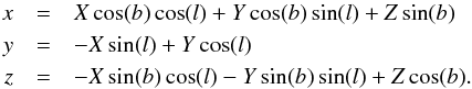 (A.1)For observations at b = 0°, we are looking directly into the Galactic plane and thus the line-of-sight coordinate, x, is entirely in the plane and the x–y plane is coincident with the X–Y plane. In this case, the z-component is equivalent to the Z-component, which is intrinsic to the particular magnetic field model being used (i.e., for Sun et al. (2008), BZ = Bz = 0, but for JF12, BZ = Bz ≠ 0). For non-zero Galactic latitudes, the x–y plane is tilted with respect to the X–Y plane by the angle b. This introduces a projected Bz −component that depends solely on the line-of-sight component. In particular, for longitudes where the magnetic field is primarily along the line of sight (e.g., l = 50°, see Fig. 1) Bx is maximum and By is close to zero. The Bz-component is exactly zero at b = 0° but it increases rapidly as | b | increases and the azimuthal component gets projected onto the plane of the sky. For longitudes where the line-of-sight component is close to zero (e.g., l = 170° and l = 355°, see Fig. 1), Bx and Bz are close to zero and By is a maximum. The By-component is perpendicular to the rotation, and thus does not get projected.
Appendix B: Hammurabi code
We use the Hammurabi code8 (Waelkens et al. 2009), which has been used previously to model the large-scale structure of the GMF. The Hammurabi code models the synchrotron emission and Faraday Rotation given an input 3D magnetic field, thermal electron distribution, and CRE distribution. The code was modified to transform the components of a magnetic field to the line-of-sight coordinate frame, which is critical for this work (see Sects. A and 5.1). We use the GMF model of JF12 and the thermal electron density distribution defined by the NE2001 code (Cordes & Lazio 2002), which is the same model used in JF12.
The CRE model defines the spectral index and the CRE spatial density distribution at all points in the volume. These quantities are defined separately for the region inside the model SNR bubble and for the surrounding Galactic medium. For the ambient Galaxy, we use the power law spectral index, p = −3 (defined as dN/dE~Ep) as this is the typical value used in other Galactic models and is the value adopted by JF12. For the spatial density, we use the distribution from WMAP (Page et al. 2007) since it is the default distribution available in Hammurabi. The ambient CRE distribution serves only to provide the surrounding background emission. Since all available models vary smoothly on the scale of the SNRs the choice of the specific model will not impact the SNR morphology nor will it affect our conclusions.
For the SNR, the CRE distribution is scaled according to the thermal electron distribution. That is, we assume the CRE density is compressed in the shell and that this compression is spherically symmetric around the whole shell. As discussed in Sect. 3, we use this assumption since we are investigating the role of the compressed ambient magnetic field on SNR morphology. The qualitative morphology of the isotropic case is very similar to the quasi-perpendicular CRE distribution since, in both cases, the resulting model SNRs are bright around the equatorial belt and faint at the polar caps (recall Fig. 2). A quantitative analysis, and comparison to the quasi-parallel scenario is beyond the scope of this work, but will be investigated in future work.
The Hammurabi code uses the HEALPIX pixelization scheme (Gorski et al. 2005), which divides the sky into pixels of equal areas. The angular resolution,  , is determined by setting the parameter NSIDE (where NSIDE is a power of 2). We use NSIDE = 8192, which corresponds to an angular resolution of 0.5′. The step size along the line of sight, Δr is set to 1 pc and the maximum distance along the line of sight, rmax is set to 1 kpc further than the distance to the SNR for a particular model (for example for modeling an SNR at 4 kpc, we would set rmax = 5 kpc). This assumes that the SNR dominates the emission in any given field and thus, the Galactic emission missing from behind the SNR does not affect the analysis.
Hammurabi calculates a number of quantities. For this work we analyze the total radio synchrotron emission, Stokes I, and the polarization vectors Stokes Q and Stokes U. These are expressed as (Waelkens et al. 2009): 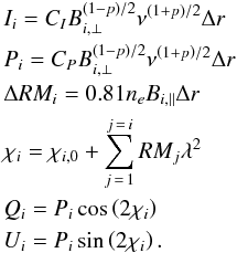 (B.1)Here, i corresponds to the ith volume element, p is the power law spectral index (see above), CI and CP are factors that are dependent on p (see Waelkens et al. 2009; Rybicki & Lightman 1979), ν is the frequency of observation, which for this work is set to 1.4 GHz, Pi is the polarized specific intensity, RM is the rotation measure, ne is the thermal electron density and λ is the wavelength of observation (0.21 m corresponds to 1.4 GHz). The total Stokes I, Stokes Q and Stokes U parameters are then found by summing the volume elements, i, along the line of sight.
Appendix C: Coordinate transformation
A coordinate transformation is used to add the SNR into the GMF for a particular location. The assumption is that a region of uniform thermal electron mass-density is transformed into a region with a mass density described by some well defined profile, which in our case is the Sedov-Taylor solution. Then, we can define two coordinate systems that describe how the thermal electron mass is distributed in these two frames and solve for the transformation that would convert from one frame to the other. The initial thermal electron mass-density distribution is uniform and the explosion occurs at a point r = 0. In this frame, the r-coordinate has uniform spacing on a numerical grid. Using conservation of mass, a new coordinate system, called r′, is defined by numerically integrating concentric spheres and comparing the mass to the uniform system. The mass of the two systems is related by 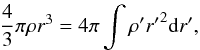 (C.1)where ρ is the thermal electron mass density in the uniform system and ρ′ is the mass density in the transformed system (i.e., the spherical shell compressed by a Sedov-Taylor blast wave).
The original uniformly distributed mass is rearranged to follow the density function defined by a standard self-similar Sedov-Taylor solution. Using the original r-coordinate (uniform density) and the new r′-coordinate (Sedov density profile) we numerically solve for a coordinate transformation matrix (Jacobian) that transforms r to the new r′-coordinate system that is given by ![Mathematical equation: \appendix \setcounter{section}{3} \begin{eqnarray} {\vec J}=\left[{\begin{array}{ccc} {\frac{{\partial x'}}{{\partial x}}} & {\frac{{\partial x'}}{{\partial y}}} & {\frac{{\partial x'}}{{\partial z}}}\\ {\frac{{\partial y'}}{{\partial x}}} & {\frac{{\partial y'}}{{\partial y}}} & {\frac{{\partial y'}}{{\partial z}}}\\ {\frac{{\partial z'}}{{\partial x}}} & {\frac{{\partial z'}}{{\partial y}}} & {\frac{{\partial z'}}{{\partial z}}} \end{array}}\right]. \end{eqnarray}](/articles/aa/full_html/2016/03/aa27001-15/aa27001-15-eq120.png) (C.2)(e.g., Boas 2005). This coordinate transformation matrix can then be applied to transform the vector field (magnetic field vectors) where
(C.2)(e.g., Boas 2005). This coordinate transformation matrix can then be applied to transform the vector field (magnetic field vectors) where  (C.3)
(C.3)
Appendix D: Data shown in comparison to the models
Figure D.1 shows data in comparison to simulated images for all modeled distances. In each case the data are shown on the left (image references are summarized in Table 3). The angle of the green-colored box was determined visually and its angle represents the bilateral axis of the data. The angle is measured from the horizontal and is set to a positive value if it is in the first quadrant, and to a negative value if it is in the second quadrant. To the right of the image is the strip of models that were made for the position of the particular SNR and at the various distances as labeled (in kpc). In some cases the Galactic field model is undefined at a location and so the model image will show blank. This affects G001.9+00.3, G003.7–0.2, G354.8–00.8 and G359.1–00.5, which are blank due to the magnetic field model being zero in central region of the Galaxy and G156.2+05.7, G166.0+04.3, and G182.4+04.3 due to the fact that the thermal electron/CRE density model is set to zero for distances beyond 17 kpc from the Galactic center. The set of best fitting models, based on the visual appearance of the angle is highlighted with an orange box, while the overall best fit model that takes all parameters into account is indicated by a green line that is drawn at the angle ψ that was measured for that particular model. Where a published value for the distance is available, the range is indicated by an arrow above the models (references for these distances are summarized in Table 3).
 |
Fig. D.1 Data (left) shown in comparison to models at distances of 0.5, 1, 2, 3, 4, 5, 6, 7, 8, 9, and 10 kpc (left to right). The angle of the green-colored box is shown at the bilateral axis angle, ψ, for the data. The set of best fitting models, based on the visual appearance of the angle is highlighted with an orange box, while the overall best fit model that takes all parameters into account is indicated by a green line that is drawn at the angle, ψ, that was measured for that particular model. In some cases the model is undefined at a location and so the model image will show blank. Where a published value for the distance is available, the range is indicated by an arrow above the models (references for these distances are summarized in Table 3). |
 |
Fig. D.1 continued. |
 |
Fig. D.1 continued. |
 |
Fig. D.1 continued. |
All Tables
Summary of the physical and angular sizes for the model SNRs bubbles at the various distances.
All Figures
|
Fig. 1 Plots of the magnetic field from JF12. Top panel: top view of the X–Y plane of the Galaxy cut through Z = 0. The green arrows show the x–y coordinate system for SNR G296.5+10.0. The dashes on the x-axis are marked at 1 kpc intervals. The purple, dashed arrows show other longitudes, l = 55°, where the GMF is primarily along the line of sight and l = 170° and l = 355°, where the GMF is primarily perpendicular to the line of sight. The filled, red circle marks the Galactic center and the filled, green circle marks the position of the Sun. Center panel: X–Z plane cut through Y = 0. As in the top panel, the filled, red circle marks the Galactic center and the filled, green circle marks the position of the Sun. The shape of the X-field can be seen. Bottom panel: GMF lines are shown as cut along l = 296.5°. Here the horizontal axis of this plot is in the X–Y plane of the Galaxy along l = 296.5°. The vertical axis of this plot shows the z-axis of the Galaxy. As in the top panel, the green arrows show the primed coordinate system, in this case the x–z coordinates, for the case of SNR G296.5+10.0, which has b = 10.0°. The dashes on the x-axis are marked at 1 kpc intervals as in the top panel. Here, one can see that for d = 1 kpc, the GMF vectors are nearly pointed along the z-axis. |
| In the text | |
|
Fig. 2 Geometry of CRE distributions for quasi-perpendicular shocks (top), quasi-parallel shocks (middle), and the isotropic case (bottom) and the corresponding simulated synchrotron emission, which has been normalized for display purposes. This cartoon is intended to qualitatively show the distribution of the CREs with respect to the magnetic field geometry. It is not intended to be representative of the precise quantitative distributions. |
| In the text | |
|
Fig. 3 Illustration of the technique used to determine the coordinate transformation matrix (Jacobian) and using it to transform the magnetic field vectors. The model uses the values from the NE2001 thermal electron density model (both local to the SNR and elsewhere along the line of sight). The technique assumes that the initial thermal electron mass density is constant locally around the SNR, which is approximately true for the NE2001 model. |
| In the text | |
|
Fig. 4 Position of the 33 SNRs in our sample showed plotted on the Galaxy with field vectors from JF12 drawn for z = 0, b = 0. The Sun’s position shown is at −8.5 kpc from the Galactic center. The thin lines represent the distance estimate from the literature while the thicker, lighter colored lines represent the best fit distance from the models. |
| In the text | |
|
Fig. 5 Top: models at the position of G317.3–00.2 and for a distance of 2 kpc showing the impact of excluding the various magnetic field components. Bottom: corresponding magnetic field vectors shown in the z–y plane (i.e., the plane of the sky, see Appendix A) and cut through the center of the SNR bubble. Left panel: only the disk field, Bdisk has been included. The two limbs are more or less uniform in brightness (slightly brighter in the north). Center panel: toroidal halo field, Btor has been included. There is now some asymmetry introduced since the magnetic field is stronger in the south with the addition of the toroidal halo component. Right panel: the X-field, BX−field, has now been included. The vector sum of these components has now made the field in the northern half of this SNR much smaller in magnitude and the direction has changed (there is now a much stronger line-of-sight (x) component in the northern half, though that is not visible on this figure). Thus the model SNR shows a high degree of asymmetry, which strongly resembles the data. |
| In the text | |
|
Fig. 6 Histogram of the differences, ψmodel−ψdata, for the best fitting models of JF12 (top) and Sun et al. (2008) (bottom). In the case of JF12, out of 33 SNRs, 25 have a difference that is < 10°, which are in agreement within our uncertainty. In the case of Sun et al. (2008), only 10 SNRs have a difference that is < 10°. |
| In the text | |
|
Fig. 7 Comparison of SNR models for three example SNRs: G296.5+10.0 (high-latitude), G016.2-2.7 (mid-latitude), and G046.8-0.3 (in the plane). All models from 0.5 to 10 kpc are shown (as described in Fig. D.1) for both GMF models: the Sun et al. (2008) (Sun08) and JF12. The orange box highlights the best fit in each case. Below the model strips we show the data (left) as well as the corresponding best fit model for JF12 (center) and Sun08 (right) . The model polarization magnetic field vectors are overlaid in green. |
| In the text | |
|
Fig. 8 Simulated polarization vectors for SNRs where observations show that they have mixed magnetic fields. These are all shown for a distance of 4 kpc, which is the best-fit distance for G054.4–0.3 and G116.9+0.2. In the case of G021.8–0.6, the best fit distance is at 5 kpc. The magnetic field at that distance is tangential, but at 4 kpc, which is still a reasonable fit, the field shows more characteristics of being mixed. |
| In the text | |
|
Fig. D.1 Data (left) shown in comparison to models at distances of 0.5, 1, 2, 3, 4, 5, 6, 7, 8, 9, and 10 kpc (left to right). The angle of the green-colored box is shown at the bilateral axis angle, ψ, for the data. The set of best fitting models, based on the visual appearance of the angle is highlighted with an orange box, while the overall best fit model that takes all parameters into account is indicated by a green line that is drawn at the angle, ψ, that was measured for that particular model. In some cases the model is undefined at a location and so the model image will show blank. Where a published value for the distance is available, the range is indicated by an arrow above the models (references for these distances are summarized in Table 3). |
| In the text | |
|
Fig. D.1 continued. |
| In the text | |
|
Fig. D.1 continued. |
| In the text | |
|
Fig. D.1 continued. |
| In the text | |
Current usage metrics show cumulative count of Article Views (full-text article views including HTML views, PDF and ePub downloads, according to the available data) and Abstracts Views on Vision4Press platform.
Data correspond to usage on the plateform after 2015. The current usage metrics is available 48-96 hours after online publication and is updated daily on week days.
Initial download of the metrics may take a while.