| Issue |
A&A
Volume 587, March 2016
|
|
|---|---|---|
| Article Number | A54 | |
| Number of page(s) | 8 | |
| Section | Stellar structure and evolution | |
| DOI | https://doi.org/10.1051/0004-6361/201526881 | |
| Published online | 16 February 2016 | |
SuperWASP discovery and SALT confirmation of a semi-detached eclipsing binary that contains a δ Scuti star
1 Department of Physical Sciences, The Open University, Walton Hall, Milton Keynes, MK7 6AA, UK
e-mail: This email address is being protected from spambots. You need JavaScript enabled to view it.
2 Astrophysics Group, Keele University, Staffordshire ST5 5BG, UK
3 Department of Physics, University of Warwick, Coventry CV4 7AL, UK
Received: 3 July 2015
Accepted: 12 January 2016
Abstract
Aims. We searched the SuperWASP archive for objects that display multiply periodic photometric variations.
Methods. Specifically we sought evidence for eclipsing binary stars that display a further non-harmonically related signal in their power spectra.
Results. The object 1SWASP J050634.16–353648.4 has been identified as a relatively bright (V ~ 11.5) semi-detached eclipsing binary with a 5.104 d orbital period that displays coherent pulsations with a semi-amplitude of 65 mmag at a frequency of 13.45 d-1. Follow-up radial velocity spectroscopy with the Southern African Large Telescope confirmed the binary nature of the system. Using the phoebe code to model the radial velocity curve with the SuperWASP photometry enabled parameters of both stellar components to be determined. This yielded a primary (pulsating) star with a mass of 1.73 ± 0.11 M⊙ and a radius of 2.41 ± 0.06 R⊙, as well as a Roche-lobe filling secondary star with a mass of 0.41 ± 0.03 M⊙ and a radius of 4.21 ± 0.11 R⊙.
Conclusions. 1SWASP J050634.16–353648.4 is therefore a bright δ Sct pulsator in a semi-detached eclipsing binary with one of the largest pulsation amplitudes of any such system known. The pulsation constant indicates that the mode is likely a first overtone radial pulsation.
Key words: binaries: eclipsing / stars: variables: delta Scuti
© ESO, 2016
1. Introduction
SuperWASP (Pollacco et al. 2006) is the world’s leading ground-based survey for transiting exoplanets. As a spin-off from its main science, it provides a long baseline, high cadence, photometric survey of bright stars across the entire sky, away from the Galactic plane. Operating since 2004, the archive contains over 2000 nights of data, comprising light curves of over 30 million stars in the magnitude range ~ 8−15, with typically 10 000 observations per object. It therefore provides a unique resource for studies of stellar variability (e.g. Norton et al. 2007; Smalley et al. 2011; 2014; Delorme et al. 2011; Lohr et al. 2013; 2014a,b, 2015a,b; Holdsworth et al. 2014). SuperWASP data is pseudo V-band, with 1 count s-1 equivalent to V ~ 15. Since the individual SuperWASP telescopes have a small aperture (11 cm), the data are subject to significant noise and uncertainties, but the long baseline and frequent observations are able to compensate for these limitations to some extent.
Stellar systems containing two or more underlying “clocks” are usually interesting objects to study and can provide critical insight into various aspects of stellar astrophysics. Zhou (2014) provides a catalogue of “oscillating binaries” of various types that includes 262 pulsating components in eclipsing binaries (96 of which contain δ Sct stars) plus a further 201 in spectroscopic binaries (including 13 δ Sct stars) and 23 in visual binaries (including one δ Sct star). They list a number of open questions that may be addressed by such systems, including the influence of binarity on pulsations and the link between them. More specifically, Liakos et al. (2012), updated in Liakos & Niarchos (2015), recently published a summary of 107 eclipsing binary systems that include a pulsating δ Sct component. They emphasise that single δ Sct stars exhibit different evolutionary behaviour to their counterparts in binary systems, which is likely related to mass transfer and tidal distortions occurring in the binaries. Since only around 100 δ Sct stars are known in eclipsing binaries, any newly identified system is noteworthy, particularly if it is bright enough for follow-up using modest instruments and if it displays a behaviour at the extremes of the rest of the sample.
2. SuperWASP data
To search for further examples of pulsating stars in binary systems, we investigated the SuperWASP archive. Previously we carried out a period-search across the entire SuperWASP data set (for details of the method employed, see Norton et al. 2007) and preliminary catalogues of eclipsing binaries and pulsating stars are presented in the Ph.D. Thesis by Payne (2012). Owing to the many systematic sources of noise in the data, the period-searching carried out typically results in multiple apparently significant periods being allocated to each object, many of which turn out to be spurious on individual investigation, since the spurious periods are usually close to harmonics of one day or one month and may be eliminated.
The approach taken here was to perform an automated search through all the potential periods identified in each SuperWASP object, picking out systems that had more than one period with high significance and for which the periods identified were not harmonically related to one another. Care was also taken to exclude periods related to each other by daily aliases, or harmonics of those aliases. Having done this, systems were identified which contained pairs of significant periods that were unrelated to each other, and thus likely represented two independent clocks in the system.
A candidate eclipsing binary that contains a pulsating star was identified and is the subject of this research. The coordinates of 1SWASP J050634.16–353648.4 (=TYC 7053–566–1) are reflected in its name, which is derived from its location in the USNO-B1 catalogue. This is an anonymous 11th magnitude star (V = 11.514,B = 11.767) that is clearly isolated both in the SuperWASP images and sky survey images. The SuperWASP photometric data comprise 56093 data points spanning over seven years from 2006 September 14 to 2013 December 6 (Fig. 1).
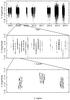 |
Fig. 1 Light curve of the SuperWASP data of 1SWASP J050634.16-353648.4, which contains over 56 000 data points, spanning seven years. Upper panel: complete dataset (with no error bars as they would obscure the data at this scale), illustrating the long term coverage; the middle panel contains a representative month’s worth of data from late 2007 (again with no error bars), illustrating that regular observations occur on most nights during an observing season and showing hints of the longer-term modulation owing to the eclipsing binary; lower panel: three nights of data and shows the observed pulsation, including error bars. |
We carried out a power spectrum analysis of the light curve using an implementation of the clean algorithm (Högbom 1974; Roberts et al. 1987) by Lehto (1993). This version utilises variable gain, thereby rendering it less susceptible to falsely cleaning out a genuine periodic signal when the data are particularly noisy. The resulting power spectrum shows two distinct sets of signals (Fig. 2). The first comprises a strong peak, which corresponds to a frequency of 1.5570803(1) × 10-4 Hz along with its first harmonic. Sidebands to each, at ± 1 sidereal day, remain even after moderate cleaning. There is a second set of frequency components with a primary period around 5.104 d, although the first harmonic at half the period is the stronger peak, and all harmonics up to 14 × the fundamental frequency can be seen.
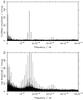 |
Fig. 2 Power spectrum of the SuperWASP data of 1SWASP J050634.16–353648.4. Lower panel: raw power spectrum, upper panel: cleaned power spectrum, both with amplitudes in mmag. Strong peaks at frequencies of 1.557 × 10⁻⁴ Hz (or 13.45 d-1) and 2.268 × 10⁻⁶ Hz (or a period around 5.104 d) are seen. |
Folding the data at the shorter period reveals a quasi-sinusoidal pulsation, but with a significant scatter that is caused by the variability at the other, longer period. To separate the two signals, a template pulsational light curve was first obtained as follows. The folded data were divided into 100 phase bins. The optimally-weighted average flux in each bin was calculated as the inverse variance-weighted mean of all the fluxes in the bin (e.g. Horne 2009). A spline curve was then interpolated through these binned average points to create a template pulse profile. Copies of this template were then subtracted from the original light curve to leave a residual light curve that we observed as being characteristic of an eclipsing binary. We then carried out a phase dispersion minimization analysis (e.g. Schwarzenberg-Czerny 1997) on the resulting light curve and identified the longer period more precisely as 5.104238(5) d. A template for the eclipsing binary light curve was then constructed from these residual phase-binned data using the optimally-weighted average flux for each bin, as before, and then fitting a spline curve to the eclipse profile. A cleaner light curve for the pulsator was then obtained by subtracting this eclipsing binary template from the full original data set. The whole procedure of creating optimally-weighted average profiles for each of the two modulations and subtracting them in turn from the original light curve was iterated a few times to ensure convergence on representative light curves and periods. The procedure was halted when the resulting folded light curves were indistinguishable from those of the previous iteration, within the data uncertainties. The final separated data, folded at the identified periods, are shown in Fig. 3 with the binned profile overlaid as a red line in each case.
Log of SALT observations.
The semi-amplitude of the pulsation is 65 ± 7 mmag, and the primary eclipses have a depth of 195 ± 7 mmag. However, since each of these amplitudes is measured from a folded light curve that has had the other modulation removed from it, there may be some systematic uncertainty in these values.
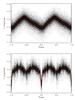 |
Fig. 3 The SuperWASP data of 1SWASP J050634.16–353648.4, folded at the pulsation period of 1.78396567 h (top) and the binary orbital period of 5.104238 d (bottom). In each case, the mean-binned light curve folded at the other period has been removed from the data. Phase zero corresponds to the minimum of the pulse in the upper panel and the primary eclipse in the lower panel; the red solid line shows the binned profile in each case. |
The times of primary minima for the eclipses may be represented by  where the figures in parentheses represent the uncertainties in the last digits. Over the seven year baseline that is available, this displays no measurable evidence for eclipse-timing variations that might indicate a secular period change or the presence of a third body in the system. The primary and secondary eclipses are separated by precisely half the orbital cycle, indicating an eccentricity, e, of zero.
3. Spectroscopic data
To confirm the nature of the system, we obtained a set of fifteen spectra of 1SWASP J050634.16–353648.4 via queue-scheduled observing on ten visits between December 2014 and February 2015 using the Southern African Large Telescope (SALT: Buckley et al. 2006). Observations were obtained using the Robert Stobie Spectrograph (RSS: Burgh et al. 2003) with the pg2300 grating, giving a dispersion of 0.17 Å per pixel in the wavelength ranges 3896−4257 Å, 4278–4623 Å, and 4642−4964 Å across the three chips of the detector. An observation log is given in Table 1. The spectra were reduced using standard iraf tools (Tody 1986; 1993) and an example spectrum is shown in Fig. 4.
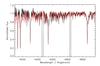 |
Fig. 4 A normalised SALT spectrum of 1SWASP J050634.16–353648.4, taken close to orbital phase zero. The red line shows the best-matching phoenix template, which has T = 7000 K and log g = 4.0. Most of the deep absorption lines are Balmer lines from Hβ to Hϵ. |
The spectra revealed two sets of lines that correspond to the two components of the system. Radial velocities for each component were measured from all spectra (except those close to phase zero where only single blended lines are seen) by cross-correlation with a best-matching template from the phoenix synthetic stellar library (Husser et al. 2013). Orbital phases and radial velocities from cross-correlating each spectrum are listed in Table 1. The template used had an effective temperature of 7000 K and solar abundances, which correspond to spectral type around F1. In the wavelength region covered by the RSS in these observations, the spectrum of 1SWASP J050634.16–353648.4 is dominated by the light from the primary star, so this is appropriate.
4. Modelling the system
We modelled 1SWASP J050634.16–353648.4 by a combination of spectral disentangling using korel (Hadrava 2004; 2012) and the phoebe interface (Prša & Zwitter 2005) to the Wilson-Devinney code (Wilson & Devinney 1971).
To work successfully, korel requires that the margins of the wavelength region in the analysed spectra contain only continuum with no spectral lines. There was no such extended region at the extremes of our spectra so we used seven separate wavelength ranges, each containing several lines with continuum on either side. The seven short spectral regions were independently analysed to find K1 (the semi-amplitude of the primary component) and q (the mass ratio M2/M1), using the estimates found from cross-correlation as a starting point. All converged on very similar values, giving means of q = 0.236 ± 0.004 and K1 = 28.1 ± 0.5 km s-1. Figure 5 shows the shape of the parameter space around this location and the limited correlation between the two converged parameters. From these, K2 = 118.8 km s-1 may be derived, implying asini = 14.8 ± 0.3 R⊙. Radial velocities were also obtained for each exposure from the best superposition of the decomposed spectra (Hadrava 2009). These are shown in the two final columns of Table 1 (after the addition of the system velocity), and agree closely with those obtained from cross-correlation, except around phase 0, where the peaks corresponding to the two components were too closely blended to give reliable results. Essentially, the disentangled spectra of the primary look the same as those of the combined spectra, whilst those of the secondary are quite noisy owing to the relative faintness of that component (of order one magnitude fainter than the primary).
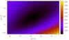 |
Fig. 5 Joint confidence levels for the mass ratio q (vertical axis) and primary semi-amplitude K1 (horizontal axis) resulting from korel. The colour scale indicates the relative goodness of fit, with darker blue corresponding to a better fit. |
In phoebe, the radial velocities from cross-correlation (excluding those near to phase 0) were used for subsequent modelling, so that a system velocity γ could be determined. The values of mass ratio and asini (with i set to 90°) were also converged as a check on those found by disentangling, giving results of q = 0.20 ± 0.02 and asini = 15.1 ± 0.4 R⊙. Since the mass ratios found by each method were significantly different, the value found from disentangling was preferred as being derived from a larger data set and consistent over different spectral regions. The values of asini and γ were then reconverged, with fixed q, simultaneously in phoebe, giving 15.2 ± 0.3 R⊙ and − 33.9 ± 1.5 km s-1, respectively, (uncertainties here are formal errors from the fit to radial velocity curves alone, but are comparable to that found for asini from korel).
Following a similar approach to that of Chew (2010), which we also used in Lohr et al. (2014a), after finding the parameters to which radial velocity curves are sensitive, the (unbinned) full SuperWASP photometric data were used to determine the angle of inclination (i), the Kopal potentials (Ω1 and Ω2), and the temperature ratio of components (T1/T2), to which light curves are primarily sensitive. (The very different quantities and qualities of our two main data sources would have skewed our results if simultaneous fitting had been attempted.) Although a range of different fitting modes were trialled, only Wilson & Devinney’s Mode 5 (semi-detached binary with secondary filling Roche lobe) reproduced both the eclipse depths and the out-of-eclipse variation with any degree of success. Therefore the secondary Kopal potential (Ω2) did not need to be determined, since it would be fixed to the value of its Roche lobe. The primary temperature T1 was also fixed to 7000 ± 200 K from our initial spectral fitting (although this had been done using composite spectra, the disentangled spectral regions for the dominant primary component were very similar to those for the combined spectrum). Other modelling assumptions were: zero eccentricity (since, as noted earlier, the eclipse spacing and durations supported a circular orbit); solar metallicities; surface albedos of 1.0; gravity brightening exponent of 1.0 for the primary (radiative atmosphere) and 0.32 for the secondary (default for convective atmosphere); and a square-root law for limb darkening. The limb darkening parameters were automatically computed by phoebe using the T and log g values to interpolate in tables from van Hamme (1993).
Using a guideline of Wilson (1994), that the ratio of eclipse depths equals the ratio of eclipsed star surface brightnesses, and that the latter gives a non-linear measure of the components’ temperature ratio, T2 was initially set to 4500 K to give a surface brightness ratio comparable to the eclipse depth ratio. Then i, T2, and Ω1 were varied over a wide-spaced grid of plausible values in a heuristic scan, and the goodness of fit was evaluated for each combination. This search revealed only one region of parameter space that corresponded to acceptable fits, within which a number of local minima are seen, two of which have very similar depths (see Fig. 6). The first of these minima (with i ~ 72°, T2 ~ 4150 K and Ω1 ~ 8.1) gives a slightly better fit to the photometric light curve out of eclipse, but a much poorer fit during the primary and secondary eclipses, whereas the second minimum (with i ~ 71°, T2 ~ 4300 K, and Ω1 ~ 6.7) gives a better fit to the photometric light curve overall, and so is preferred. To determine the uncertainties on these parameters, we selected 21 sub-samples of the photometric light curve at random (each containing 10 000 data points) and found the best fit to each of these sub-datasets in conjunction with the radial velocity data. The distributions of the best fit values for the i, T2, and Ω1 parameters were then used to assign error bars to each parameter, which represent the standard deviation or one-sigma confidence levels. This, in turn, allowed us to assign confidence levels to the contours in Fig. 6, as shown by the colour bars. Optimal values for i, T2, and Ω1 were finally obtained by simultaneous convergence within phoebe. After each iteration, the value of a was recalculated to maintain asini at the value previously found from the radial velocity curves. This procedure gave values as shown in Table 2; uncertainties are formal errors from the fit, except for those of i, T2, and Ω1, which were determined from the procedure described above.
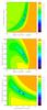 |
Fig. 6 Joint confidence levels for pairs of parameter values (i, T2, and Ω1 in various combinations) obtained from a series of heuristic scans over a grid around the best fit region. Darker colours correspond to better fits, as indicated by the colour bar; the numerical values represent the number of standard deviations away from the best-fit value. |
The output values from the modelling (absolute masses, radii, bolometric magnitudes, and surface gravities) are also shown in Table 2. The uncertainties in the masses were obtained using the formulae prescribed in the phoebe manual, and are dominated by the uncertainty in the semi-major axis given by the radial velocities.
The uncertainties in the other output values were found by setting relevant input parameters to their extrema in appropriate combinations, and thus may be expected to overestimate the true uncertainties slightly. The final fits to radial velocity and light curves, with their residuals, are shown in Figs. 7 and 8, and images of the best-fitting model at two phases are presented in Fig. 9, revealing the substantial ellipsoidal distortion of the secondary.
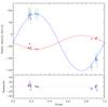 |
Fig. 7 Radial velocity curves of the two components of 1SWASP J050634.16–353648.4. The best-fitting model from phoebe is over-plotted showing the motion of the primary (red) and secondary (blue). Lower panel: residuals between the fit and the data, revealing no systematic trends. |
System parameters for 1SWASP J050634.16–353648.4.
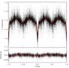 |
Fig. 8 Eclipsing binary light curve for 1SWASP J050634.16–353648.4, over-plotted with the best-fitting model from phoebe. The lower panel shows the residuals between the model fit and the binned data (which we emphasize was not used in the modelling). Around ingress to, and egress from, the primary eclipse, the rapid changes are not as well sampled by the SuperWASP data as in the out-of-eclipse regions, and so give rise to slightly higher residuals of order 0.01 mag. |
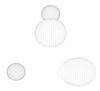 |
Fig. 9 Schematic diagrams of 1SWASP J050634.16–353648.4 at phases 0 and 0.25, according to the best fitting model from phoebe. |
For comparison with the parameters we have derived, we note that elsewhere 1SWASP J050634.16–353648.4 is included as HE0504–3540 in the catalogue of metal-poor stars from the Hamburg/ESO objective prism survey (Christlieb et al. 2008), where it is listed as having an estimated [Fe/H] value of between –2.1 and –2.9 and a negligible interstellar reddening of E(B−V) = 0.01. We note, however, that these metallicity values may be affected by the composite nature of the spectrum.
In the fourth data release of the rave experiment (Kordopatis et al. 2013), 1SWASP J050634.16–353648.4 is listed as having an effective temperature of 6227 K and log g = 1.82 with a metallicity of − 0.06. Since the rave spectra are obtained in the infrared (8410−8794 Å), where the cooler secondary star will make a significant contribution to the overall spectrum, these parameters are clearly composite values for the unresolved binary.
5. Discussion
5.1. Pulsation analysis
Although the photometric data span over seven years and comprise more than 56 000 data points, they are, nonetheless, obtained using 11 cm aperture telescopes from a ground-based site. Consequently, the data do not permit the sort of detailed frequency analyses that have been carried out on similar pulsating stars in eclipsing binaries using data from Kepler and CoRoT (e.g. Hambleton et al. 2013; da Silva et al. 2014). Nonetheless, we have subtracted the mean orbital modulation from the light curve and then performed a clean analysis of the resulting detrended data to search for pulsational frequency components. The only frequency components remaining in the power spectrum above the amplitude noise threshold of ~ 2 mmag are the fundamental pulsation frequency and its first harmonic (along with ± 1 sidereal day sidebands for each). The amplitude of the first harmonic is 15% that of the fundamental frequency, and the relative phasing between them is such that the fundamental leads the first harmonic by about 60°.
Using the relationship between the pulsation frequency of a given radial mode fpulse, the pulsation constant Q and the ratio of the mean density of the star to that of the Sun 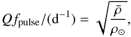 we see that, for the observed fundamental frequency of 13.45 d-1, the pulsation constant is Q = 0.026 ± 0.002. Alternatively, using the relation from Breger et al. (1993), which is adapted from that in Petersen & Jorgensen (1972)
  we also calculate Q = 0.026 ± 0.002. According to Stellingwerf (1979) this is typical of a first overtone (n = 1) radial pulsation in a δ Sct star with the parameters we have modeled here, and similarly Petersen & Jorgensen (1972) derive a theoretical pulsation constant of Q1 = 0.0252 for the first overtone radial mode, in agreement with our calculated value.
We note the period-luminosity relation for short-period pulsating stars derived by Poretti et al. (2008):  Using our observed value for the observed pulsation period of 0.0743 d, yields MV = 2.29 ± 0.16, which is in excellent agreement with the bolometric luminosity derived from the phoebe model fit (Table 2), thereby lending further support for the interpretation.
The absence of any pulsation frequencies in the detrended power spectrum at multiples of the orbital frequency indicates that we do not detect any tidally excited modes. However, given that the orbit is apparently circular, this is to be expected.
5.2. In context with other systems
The parameters of 1SWASP J050634.16–353648.4 are remarkably similar to those of the star UNSW–V–500 which was announced by Christiansen et al. (2007) as the first high-amplitude δ Scuti (HADS) star in an eclipsing binary system. That too is a semi-detached system in a 5 d orbit with primary and secondary masses and radii of 1.49 M⊙ + 0.33 M⊙, and 2.35 R⊙ + 4.04 R⊙, respectively. Temperatures, surface gravities, and bolometric luminosities are also similar between the two systems, although the pulsational amplitude of UNSW–V–500 is about five times larger than that of 1SWASP J050634.16–353648.4, as discussed below. Nonetheless, UNSW–V–500 also pulsates in the single first overtone radial mode, with a pulsation constant of Q = 0.025 ± 0.004, which is again the same as that of our target.
Liakos & Niarchos (2015), in an update to Liakos et al. (2012), list 107 objects as eclipsing binaries that contain δ Sct stars. Only four of those on the original list from Liakos et al. (2012), namely KW Aur, TZ Eri, BO Her, and MX Pav, have comparable or larger pulsational semi-amplitudes to our object, being in the range 68–83 mmag. However, 1SWASP J050634.16–353648.4 is not regarded as a HADS star, as such a designation is reserved for those with pulsational semi-amplitudes in excess of 300 mmag. Only two HADS stars in eclipsing binaries are known: the star UNSW-V-500 (Christiansen et al. 2007), with a semi-amplitude of 350 mmag, and RS Gru (Derekas et al. 2009), with a semi-amplitude of 600 mmag. All HADS stars typically have dominant pulsations in the fundamental radial mode (McNamara 2000), although some double-mode systems also pulsate in the first and second overtone radial modes. Unusually, UNSW-V-500, like our target, is a single-mode field star pulsating only in the first overtone radial mode.
Liakos & Niarchos (2015) present a convincing empirical correlation between the orbital period and pulsation period of all δ Sct stars in eclipsing binaries with Porb< 13 d:
 The periods of 1SWASP J050634.16–353648.4, namely Ppulse = 0.0743 d and Porb = 5.104 d, fit this relationship perfectly: a pulse period of (0.075 ± 0.003) d is predicted, based on the orbital period, and an orbital period of (5.0 ± 0.4) d is predicted, based on the pulse period. Our object thus lends further support to their empirical fit. Although we note that the parameters of two recently described systems with high-quality space-based photometry – KIC 4544587 (Hambleton et al. 2013) and CoRoT 105906206 (Da Silva et al. 2014) – do not follow the proposed relation.
Liakos & Niarchos (2015) also show that the pulse periods of δ Sct stars in binary systems are correlated with their surface gravity according to
 Once again, this fits perfectly with 1SWASP J050634.16–353648.4, predicting log g = 4.0 ± 0.2 for the pulsating star, in line with that observed.
5.3. Evolutionary state
The semi-detached configuration implied by the results of the phoebe modelling indicates that mass transfer may be a possibility in 1SWASP J050634.16–353648.4. However, we see no evidence for current mass transfer in either the photometry or spectroscopy. The heights of the maxima in the binary light curve are the same, indicating that there are unlikely to be significant spotted regions on either component. There is no long-term period change detected over the seven year baseline. There are no emission lines seen in the spectrum and there is no X-ray emission seen in the ROSAT All Sky Survey that is coincident with the location of this object, the nearest X-ray source being 14 arcmin away. Each of these reasons point to negligible mass transfer currently occurring.
Mkrtichian et al. (2004) introduced the classification of oEA (oscillating EA) binaries for eight systems that are classified as Algol-type eclipsing binaries with mass accreting pulsating components (i.e. Y Cam, AB Cas, RZ Cas, R CMa, TW Dra, AS Eri, RX Hya, and AB Per). Amongst the eclipsing binaries with δ Sct components listed by Liakos & Niarchos (2015), over half are listed as semi-detached, but it is not clear in what proportion of them mass transfer is currently occurring.
In Fig. 10 we show a mass-radius plot, which illustrates the position of 1SWASP J050634.16–353648.4, along with that of UNSW-V-500 for comparison. These are overplotted on Dartmouth model isochrones (Dotter et al. 2008), revealing that the δ Sct star in our target is somewhat younger than that in UNSW-V-500, in the range 1.1−1.8 Gy. (The companion, non-pulsating stars, in each system are not plotted, since they fill their Roche lobes and so their radii do not represent the size of the corresponding single star.) We also note that, in the presence of possible mass transfer between the two components of each system, the use of single star tracks for the pulsating components may also misrepresent their ages.
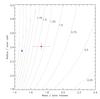 |
Fig. 10 A mass-radius plot showing the positions of 1SWASP J050634.16–353648.4 (red diamond) and UNSW-V-500 (blue triangle) over-plotted on Dartmouth model isochrones, with ages indicated in Gy. |
6. Conclusion
We can confirm that 1SWASP J050634.16–353648.4 is a δ Sct star with a 65 mmag semi-amplitude, 1.784 h pulsation in an eclipsing binary, whose orbital period is 5.104 d. The primary has a mass and radius of 1.7 M⊙ and 2.4 R⊙ with log g = 3.9 and is around spectral type F1 with an age of ~ 1.1−1.8 Gy; the secondary fills its Roche lobe with a mass and radius of 0.4 M⊙ and 4.2 R⊙ with log g = 2.8. The pulsation constant is Q = 0.026 ± 0.002 and indicates a first overtone radial pulsation mode; no tidally excited pulsations are apparent. The system is thus a relatively rare, long period, semi-detached eclipsing binary containing a δ Sct star with a large pulsation amplitude, similar to UNSW-V-500.
Acknowledgments
The WASP project is currently funded and operated by Warwick University and Keele University, and was originally set up by Queen’s University Belfast, the Universities of Keele, St. Andrews and Leicester, the Open University, the Isaac Newton Group, the Instituto de Astrofisica de Canarias, the South African Astronomical Observatory and by STFC. Some of the observations reported in this paper were obtained with the Southern African Large Telescope (SALT), under programme 2014-2-SCI-010 (PI: Norton), for which the Open University is a shareholder, as part of the UK SALT Consortium. One of us (Lohr) is supported under the STFC consolidated grant to the Open University, ST/L000776/1. The research made use of the SIMBAD database, operated at CDS, Strasbourg, France.
References
- Breger, M., Stich, J., Garrido, R., et al. 1993, A&A, 271, 482 [NASA ADS] [Google Scholar]
- Buckley, D. A. H., Swart, G. P., & Meiring, J. G. 2006, in Ground-based and Airborne Telescopes, ed. L. M. Stepp, Proc. SPIE, 6267, 62670 [Google Scholar]
- Burgh, E. B., Nordsieck, K. H., Kobulnicky, H. A., et al. 2003, in Instrument Design and Performance for Optical/Infrared Ground-based Telescopes, eds. M. Iye, & A. F. M. Moorwood, Proc. SPIE, 4841, 1463 [Google Scholar]
- Chew, Y. G. M. 2010, Ph.D. Thesis, Vanderbilt University [Google Scholar]
- Christiansen, J. L., Derekas, A., Ashley, M. C. B., et al. 2007, MNRAS, 382, 239 [NASA ADS] [CrossRef] [Google Scholar]
- Christlieb, N., Schörck, T., Frebel, A., et al. 2008, A&A, 484, 721 [NASA ADS] [CrossRef] [EDP Sciences] [Google Scholar]
- Delorme, P., Collier Cameron, A., Hebb, L., et al. 2011, MNRAS, 413, 2218 [NASA ADS] [CrossRef] [Google Scholar]
- Derekas, A., Kiss, L. L., Bedding, T. R., et al. 2009, MNRAS, 394, 995 [NASA ADS] [CrossRef] [Google Scholar]
- Dotter, A., Chaboyer, B., Jevremovic, D., et al. 2008, ApJS, 178, 89 [NASA ADS] [CrossRef] [Google Scholar]
- Hadrava, P. 2004, Publ. Astron. Inst. Academy of Sciences of the Czech Republic, 92, 15 [Google Scholar]
- Hadrava, P. 2009, ArXiv eprints [arXiv:0909.0172] [Google Scholar]
- Hadrava, P. 2012, in From Interacting Binaries to Exoplanets: Essential Modeling Tools, eds. M. T. Richards, & I. Hubeny, IAU Symp., 282, 351 [Google Scholar]
- Hambleton, K. M., Kurtz, D. W., Prsa, A., et al. 2013, MNRAS, 434, 925 [NASA ADS] [CrossRef] [MathSciNet] [Google Scholar]
- Högbom, J. A. 1974, A&AS, 15, 417 [NASA ADS] [Google Scholar]
- Holdsworth, D. L., Smalley, B., Gillon, M., et al. 2014, MNRAS, 439, 2078 [NASA ADS] [CrossRef] [Google Scholar]
- Horne, K. D. 2009, The ways of our errors: optimal data analysis for beginners and experts, University of St Andrews, http://www-star.st-and.ac.uk/~kdh1/ada/woe/woe.pdf [Google Scholar]
- Husser, T. O., von Berg, S. W., Dreizler, S., et al. 2013, A&A, 553, A6 [NASA ADS] [CrossRef] [EDP Sciences] [Google Scholar]
- Kordopatis, G., Gilmore, G., Steinmetz, M., et al. 2013, AJ, 146, 134 [NASA ADS] [CrossRef] [Google Scholar]
- Lehto, H. J. 1993, in Proc. Int. conf. on applications of time series analysis in astronomy and meteorology, ed. O. Lessi (University of Padua Press), 99 [Google Scholar]
- Liakos, A., & Niarchos, P. 2015, ASP Conf. Ser., 496, 195 [NASA ADS] [Google Scholar]
- Liakos, A., Niarchos, P., Soydugan, E., & Zasche, P. 2012, MNRAS, 422, 1250 [NASA ADS] [CrossRef] [Google Scholar]
- Lohr, M. E., Norton, A. J., Kolb, U. C., et al. 2013, A&A, 549, A86 [NASA ADS] [CrossRef] [EDP Sciences] [Google Scholar]
- Lohr, M. E., Hodgkin, S. T., Norton, A. J., & Kolb, U. C. 2014a, A&A, 563, A34 [NASA ADS] [CrossRef] [EDP Sciences] [Google Scholar]
- Lohr, M. E., Norton, A. J., Anderson, D. R., et al. 2014b, A&A, 566, A128 [NASA ADS] [CrossRef] [EDP Sciences] [Google Scholar]
- Lohr, M. E., Norton, A. J., Gillen, E., et al. 2015a, A&A, 578, A103 [NASA ADS] [CrossRef] [EDP Sciences] [Google Scholar]
- Lohr, M. E., Norton, A. J., Payne, S. G., et al. 2015b, A&A, 578, A136 [NASA ADS] [CrossRef] [EDP Sciences] [Google Scholar]
- McNamara, D. H. 2000, in Delta Scuti and related Stars, eds. M. Breger, & M. Montgomery, ASP Conf. Ser., 210, 373 [Google Scholar]
- Norton, A. J., Wheatley, P. J., West, R. G., et al. 2007, A&A, 467, 785 [NASA ADS] [CrossRef] [EDP Sciences] [Google Scholar]
- Payne, S. G. 2012, Ph.D. Thesis, The Open University [Google Scholar]
- Petersen, J. O., & Jorgensen, H. E. 1972, A&A, 17, 367 [NASA ADS] [Google Scholar]
- Pollacco, D. L., Skillen, I., Cameron, A. C., et al. 2006, PASP, 118, 1407 [NASA ADS] [CrossRef] [Google Scholar]
- Poretti, E., Clementini, G., Held, E. V., et al. 2008, ApJ, 685, 947 [NASA ADS] [CrossRef] [Google Scholar]
- Prša, A., & Zwitter, T. 2005, ApJ, 628, 426. [NASA ADS] [CrossRef] [Google Scholar]
- Roberts, D. H., Lehár, J., & Dreher, J. W. 1987, AJ, 93, 968 [NASA ADS] [CrossRef] [Google Scholar]
- Schwarzenberg-Czerny, A. 1997, ApJ, 489, 941 [NASA ADS] [CrossRef] [Google Scholar]
- da Silva, R., Maceroni, C., Gandolfi, D., et al. 2014, A&A, 565, A55 [NASA ADS] [CrossRef] [EDP Sciences] [Google Scholar]
- Smalley, B., Kurtz, D. W., Smith, A. M. S., et al. 2011, A&A, 535, A3 [CrossRef] [EDP Sciences] [Google Scholar]
- Smalley, B., Southworth, J., Pintado, O. I., et al. 2014, A&A, 564, A69 [NASA ADS] [CrossRef] [EDP Sciences] [Google Scholar]
- Stellingwerf, R. F. 1979, ApJ, 227, 935 [NASA ADS] [CrossRef] [Google Scholar]
- Tody, D. 1986, in Instrumentation in astronomy VI, ed. D. L. Crawford, SPIE Conf. Ser., 627, 733 [Google Scholar]
- Tody, D. 1993, in Astronomical Data Analysis Software and Systems II, eds. R. J. Hanisch, R. J. V. Brissenden, & J. Barnes, ASP Conf. Ser., 52, 173 [Google Scholar]
- van Hamme, W. 1993, AJ, 106, 2096 [NASA ADS] [CrossRef] [Google Scholar]
- Wilson, R. E. 1994, International Amateur-Professional Photoelectric Photometry Communication, 55, 1 [NASA ADS] [Google Scholar]
- Wilson, R. E., & Devinney, E. J. 1971, ApJ, 166, 605 [NASA ADS] [CrossRef] [Google Scholar]
- Zhou, A-Y. 2014, ArXiv eprints [arXiv:1002:2729] [Google Scholar]
All Tables
All Figures
|
Fig. 1 Light curve of the SuperWASP data of 1SWASP J050634.16-353648.4, which contains over 56 000 data points, spanning seven years. Upper panel: complete dataset (with no error bars as they would obscure the data at this scale), illustrating the long term coverage; the middle panel contains a representative month’s worth of data from late 2007 (again with no error bars), illustrating that regular observations occur on most nights during an observing season and showing hints of the longer-term modulation owing to the eclipsing binary; lower panel: three nights of data and shows the observed pulsation, including error bars. |
| In the text | |
|
Fig. 2 Power spectrum of the SuperWASP data of 1SWASP J050634.16–353648.4. Lower panel: raw power spectrum, upper panel: cleaned power spectrum, both with amplitudes in mmag. Strong peaks at frequencies of 1.557 × 10⁻⁴ Hz (or 13.45 d-1) and 2.268 × 10⁻⁶ Hz (or a period around 5.104 d) are seen. |
| In the text | |
|
Fig. 3 The SuperWASP data of 1SWASP J050634.16–353648.4, folded at the pulsation period of 1.78396567 h (top) and the binary orbital period of 5.104238 d (bottom). In each case, the mean-binned light curve folded at the other period has been removed from the data. Phase zero corresponds to the minimum of the pulse in the upper panel and the primary eclipse in the lower panel; the red solid line shows the binned profile in each case. |
| In the text | |
|
Fig. 4 A normalised SALT spectrum of 1SWASP J050634.16–353648.4, taken close to orbital phase zero. The red line shows the best-matching phoenix template, which has T = 7000 K and log g = 4.0. Most of the deep absorption lines are Balmer lines from Hβ to Hϵ. |
| In the text | |
|
Fig. 5 Joint confidence levels for the mass ratio q (vertical axis) and primary semi-amplitude K1 (horizontal axis) resulting from korel. The colour scale indicates the relative goodness of fit, with darker blue corresponding to a better fit. |
| In the text | |
|
Fig. 6 Joint confidence levels for pairs of parameter values (i, T2, and Ω1 in various combinations) obtained from a series of heuristic scans over a grid around the best fit region. Darker colours correspond to better fits, as indicated by the colour bar; the numerical values represent the number of standard deviations away from the best-fit value. |
| In the text | |
|
Fig. 7 Radial velocity curves of the two components of 1SWASP J050634.16–353648.4. The best-fitting model from phoebe is over-plotted showing the motion of the primary (red) and secondary (blue). Lower panel: residuals between the fit and the data, revealing no systematic trends. |
| In the text | |
|
Fig. 8 Eclipsing binary light curve for 1SWASP J050634.16–353648.4, over-plotted with the best-fitting model from phoebe. The lower panel shows the residuals between the model fit and the binned data (which we emphasize was not used in the modelling). Around ingress to, and egress from, the primary eclipse, the rapid changes are not as well sampled by the SuperWASP data as in the out-of-eclipse regions, and so give rise to slightly higher residuals of order 0.01 mag. |
| In the text | |
|
Fig. 9 Schematic diagrams of 1SWASP J050634.16–353648.4 at phases 0 and 0.25, according to the best fitting model from phoebe. |
| In the text | |
|
Fig. 10 A mass-radius plot showing the positions of 1SWASP J050634.16–353648.4 (red diamond) and UNSW-V-500 (blue triangle) over-plotted on Dartmouth model isochrones, with ages indicated in Gy. |
| In the text | |
Current usage metrics show cumulative count of Article Views (full-text article views including HTML views, PDF and ePub downloads, according to the available data) and Abstracts Views on Vision4Press platform.
Data correspond to usage on the plateform after 2015. The current usage metrics is available 48-96 hours after online publication and is updated daily on week days.
Initial download of the metrics may take a while.