| Issue |
A&A
Volume 587, March 2016
|
|
|---|---|---|
| Article Number | A5 | |
| Number of page(s) | 10 | |
| Section | Interstellar and circumstellar matter | |
| DOI | https://doi.org/10.1051/0004-6361/201526870 | |
| Published online | 11 February 2016 | |
Correlation of HI shells and CO clumps in the outer Milky Way
Astronomical Institute, Academy of Sciences,
1401 Boční II, Prague, Czech
Republic
e-mail:
sona.ehlerova@asu.cas.cz
Received: 1 July 2015
Accepted: 3 December 2015
Context. HI shells, which may be formed by the activity of young and massive stars, or connected to energy released by interactions of high-velocity clouds with the galactic disk, may be partly responsible both for the destruction of CO clouds and for the creation of others. It is not known which effect prevails.
Aims. We study the relation between HI shells and CO in the outer parts of the Milky Way, using HI and CO surveys and a catalogue of previously identified HI shells.
Methods. For each individual location, the distance to the nearest HI shell is calculated and it is specified whether it lies in the interior of an HI shell, in its walls, or outside an HI shell. The method takes into account irregular shapes of HI shells.
Results. We find a lack of CO clouds in the interiors of HI shells and their increased occurrence in walls. Properties of clouds differ for different environments: interiors of HI shells, their walls, and unperturbed medium.
Conclusions. CO clouds found in the interiors of HI shells are those that survived and were robbed of their more diffuse gas. Walls of HI shells have a high molecular content, indicative of an increased rate of CO formation. Comparing the CO fractions within HI shells and outside in the unperturbed medium, we conclude that HI shells are responsible for a ~20% increase in the total amount of CO in the outer Milky Way.
Key words: ISM: bubbles / ISM: clouds / Galaxy: structure
© ESO, 2016
1. Introduction
The interstellar medium (ISM) is full of structures on all scales, from sub-pc to kpc. The larger structures, among which the HI shells, were discovered first; the shells were found in the HI distribution ranging in sizes from a few pc to about 1 kpc. The first list of HI shells in the Milky Way was published by Heiles (1979) and others followed: McClure-Griffiths et al. (2002), Ehlerová & Palouš (2005, 2013), Suad et al. (2014). HI shells were also identified in other galaxies (for a review on shells in external galaxies and an analysis of HI shells in THINGS galaxies see Bagetakos et al. 2011).
Since early days it has been speculated that these shells are the result of energetic activities of massive stars: winds, radiation, and supernova explosions. For many large shells, the energy needed to create them must have come from the whole cluster of stars, from OB associations. Proving this connection is not completely straightforward since many shells are older than the expected lifetime of massive stars and the results are often confusing (Rhode et al. 1999; Stewart et al. 2000). However, the statistical correspondence between HI shells and stars (Ehlerová & Palouš 2013; Suad et al. 2014) indicates the relation.
Many observational papers, both for the Milky Way and external galaxies, show that HI shells frequently exist at large galactocentric distances, far from star forming regions and often with quite large sizes. This implies, that other mechanisms might be employed to explain these structures: ram pressure (Bureau & Carignan 2002) or the infall of a high-velocity cloud to the disk (Tenorio-Tagle et al. 1987). These events might be responsible for a fraction of HI shells, but probably not for the majority.
HI shells evolve in a gaseous disk. They are sensitive to local density distribution, but since they are quite big, they quickly overgrow the smaller pc scale fluctuations. Once their dimensions are comparable to the disk scale – which is not unusual – their shapes should be influenced by the large-scale density gradient in the disk and they may prolong in the z-direction (these prolonged shells are usually called worms). If the interior of the shell is still hot – i.e. if the progenitor massive stars still exist – this hot gas may flow into the galactic halo (the worms become chimneys). In such a way HI shells may influence the energetic flows in galaxies. For dwarf galaxies with low gravity (e.g. van Eymeren et al. 2009) or for starburst galaxies (e.g. M 82), such an event could mean the loss of this hot gas to the intergalactic medium.
With the advent of infrared satellites, structures with pc sizes were discovered in the dust emission. They were found to be almost everywhere in the disk and therefore we talk about the “bubbling galactic disk” (Churchwell et al. 2006; Deharveng et al. 2010; Simpson et al. 2012). However, the infrared bubbles are quite different from HI shells. Some of them are connected to young stars; basically, each massive star is able to produce an HII region, which is surrounded by the photodissociation region identified as the infrared bubble (Anderson et al. 2012). They are often found in the vicinity of CO clouds and other indicators of the on-going star formation. One might expect, that some of these bubbles – or mergers of several of these bubbles – may eventually grow to become HI shells. The bubbles discovered in the MIPSGAL 24 μ survey (Mizuno et al. 2010) may have different origins; some of them are connected to planetary nebulae and late phases of stellar evolution.
Some of the infrared bubbles, as already stated, are directly connected to the on-going (or more correctly, very recent) star formation. It is speculated that the bubbles might trigger the new star formation as their walls are the homes of objects younger than the bubble itself (Walch et al. 2015; Sidorin et al. 2014, and many more), either by the collect & collapse scenario or by radiation driven implosion. Another interpretation might be that they are only the redistributors of the star formation that would happen anyway.
For HI shells, the situation is even less clear. They are – or were – strong shocks (Tenorio-Tagle & Bodenheimer 1988) and as such we can imagine for them both the inhibiting model, i.e. the destruction of existing molecular clouds by intense radiation, strong winds, and supernova explosions, or the supporting/stimulating model, i.e. the increased cloud formation in the swept-up gas around clusters of young stars.
For small dwarf galaxies the star formation taking place mostly in the centre of the galaxy may create one supergiant HI shell, which then significantly influences the secondary star formation (as an example see the Holmberg I galaxy, Ott et al. 2001). However, the Milky Way is a large galaxy that has more complex patterns of star formation.
Dawson et al. (2013) studied the relationship between HI and CO in supergiant shells in the Large Magellanic Cloud (LMC). They found out that ~(4−10)% of the total molecular mass of the LMC was created as a by-product of the stellar activity that formed the shells. Dawson et al. (2011) studied two supershells in the Milky Way and found that both objects show an enhanced level of molecularization. Both these studies indicate the stimulating effect of supershells on the molecularization and the total amount of CO in galaxies.
Unlike the two papers mentioned, we want to study the effect of all shells, not only supershells, which are striking and important examples of an HI shell population, but are not typical. The origin of the shells and supershells may be different, and the net outcome of all shells, small and large, could differ from the outcome of supershells. We analyse the relation between CO and HI bubbles; more specifically, we discuss whether CO is concentrated in the walls of HI bubbles, whether there is little or no correlation between CO and HI bubbles, and how the position of CO in relation to HI shells influences the CO properties.
2. Data
In our analysis we use two kinds of input datacubes: HI data and CO data, and also a catalogue of HI shells by Ehlerová & Palouš (2013, Paper I). We focus on the outer parts of the Galaxy and avoid the inner parts, which are too full of HI shells and bubbles. Owing to the high filling factor of bubbles, in the inner Galaxy it is difficult to define their shapes precisely (or at least reasonably precisely; see the discussion in Paper I). Therefore, we restrict our study to the strip b ∈ (−5°, +5°) in the 2nd and 3rd Galactic quadrants: l ∈ (90°,270°).
The longitude-latitude-velocity (lbv) datacubes contain a lot of “empty space”; the signal is below the sensitivity limit because there is too little gas at a given location and velocity because the corresponding velocities are forbidden (for each quadrant about half of the cube lies at forbidden velocities), because there is no gas there (e.g. because it is too far from the Galactic centre), or because the sensitivity of the survey is simply too low. To avoid the empty lbv regions, we always study only pixels/places with some HI emission THI ≥ THIcutoff (see the next section for the choice of THIcutoff).
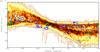 |
Fig. 1 Galactic longitude-velocity map at the Galactic latitude b = 0° of the outer Milky Way: HI (map), CO (green contours) and HI shells (blue outlines). |
2.1. HI data
We use the Leiden/Argentina/Bonn HI survey (LAB; Kalberla et al. 2005). It is an all-sky survey, a combination of observations made from two instruments. The angular resolution (HPBW) is ~ , the velocity resolution is 1.3 kms-1, and the LSR velocity covers the interval (− 450,450) kms-1. The HI datacube contains the brightness temperature; the rms noise of the LAB survey is (0.07−0.09) K.
The pixel size of the LAB datacube is 0.5° and the channelwidth is Δv = 1.0306 kms-1. As mentioned above, to avoid the empty regions of the lbv we have to define a certain cutoff of an HI emission THIcutoff. We choose the HI cutoff to be 0.3 K, which equals the 3 σ level of noise in the HI data, and which also corresponds to values chosen for the detection of HI shells (see Paper I). It corresponds to a column density of 5.5 × 1017 cm-2.
We performed some calculations with other HI cutoffs to test the dependence of our results on this value. If not otherwise stated, when we refer to ‘the studied datacube’ it means that we restrict ourselves to the parts of it that have THI ≥ 0.3 K.
2.2. CO data
We use the CO (J = 1− > 0) survey of Dame et al. (2001). It is a composite survey of the Milky Way, consisting of observations from several telescopes. It is not an all-sky survey, but it contains the whole Galactic plane and some additional regions. Resolutions, samplings, and sensivities of the different surveys vary.
The combined datacube (the so-called deep CO survey) that we use has a pixel size of 0.125° and a channelwidth of Δv = 1.3 kms-1. In the 2nd and 3rd quadrants it fully covers the Galactic plane region in the belt b ∈ (−5°, + 5°).
The datacube gives the main beam temperature; the rms noise is 0.1 K. However, probably due to the ‘drastic noise reduction’ mentioned in Dame et al. (2001), it is safer to believe only the data above ~5σ.
2.3. HI shells
As an input catalogue of HI shells we use our own catalogue from Paper I. Shells in this list were identified automatically as continuous regions of a lower HI temperature surrounded by a higher temperature wall or region. The search was done in 2D lb-maps and then the detected low-temperature regions were combined into 3D lbv structures. There were no prescriptions of the shape of the HI shell, but the structures had to span at least eight consecutive velocity channels (i.e. 8 kms-1), and their spectra had to show a temperature contrast of at least 4 K towards their surroundings. The overlap between 2D lb-cuts of the 3D lbv-structure identified in the subsequent channel maps must be large enough and they should have a similar size and shape (see Paper I for more precise discussion). The minimum angular dimension of the detected structure is  , the maximum is 45°. The algorithm cannot detect entirely open structures such as very evolved galactic chimneys or structures with completely fragmented walls (see also the discusion in Sect. 5.3). Identified structures are low-temperature regions, i.e. interiors of HI shells. Walls are not detected by our algorithm and the dimensions used here and taken from Paper I also refer only to sizes of the interiors.
The analysis of the HI LAB survey (LAB; Kalberla et al. 2005) using methods and conditions briefly summarized in the paragraph above we identified 333 shells. By looking at results and by comparing our findings with other catalogues of HI shells (McClure-Griffiths et al. 2002; Suad et al. 2014) we found that the identifications in the outer Milky Way are more reliable than identifications in the inner Milky Way, probably owing to a heavy overlapping of shells in the inner disk. This is the main reason, why in the current study we are only interested in the outer Milky Way.
The studied datacube contains the whole volume or a significant fraction of the volume of 70 HI shells from the catalogue plus some smaller parts of ten more shells. For the current analysis we use the real 3D pixel maps of shells; the idealized dimensions (Δl0, Δb0, Δv0) and positions (l0, b0, v0) of these shells are given in Table 1 of Paper I. As an example Fig. 1 shows the HI lv-map at (b = 0°) with CO contours and HI shells outlines overlaid. HI shells do not overlap significantly in the studied datacube and we see that CO avoids the internal volume of shells.
2.4. Comparing HI and CO datacubes
Pixel sizes and channelwidths of the HI and CO datacubes differ. Therefore, we construct an auxiliary grid with high resolution and for each pixel of this auxiliary grid we find the closest HI or CO pixel and their appropriate values. All grid calculations are done in this auxiliary grid. We do not interpolate the values or regrid the HI or CO datacubes, but we keep their original resolution.
This is only one possible method; we made a few calculations with datacubes regridded to the lower resolution of the two original datacubes. The results were similar to the results of our current approach.
3. Methods
Here we describe how we attribute the HI shells and their parts to studied pixels, and which quantities we are interested in.
3.1. Composition of an HI shell
An HI shell consists of an HI bubble, sometimes also called a hole, and an HI wall. A bubble is the interior of the shell, a region of lower HI temperature (i.e. density). This structure was identified by the searching algorithm in Paper I (and it is an input quantity). The wall is, from the technical point of view, a region just neighbouring the bubble.
3.2. Different types of pixels
For each pixel of the studied datacube we have to know two things: first, whether it is inside the HI bubble or not and second, how far it is from the wall of the bubble (if it lies inside it) or how far it is from the wall of the nearest HI bubble (if it is outside). We know the first from the HI shells datacube (section HI shells); we have to calculate the second from this datacube.
For pixels that do not lie inside any HI bubble, we have to find the nearest HI bubble. For each such outside pixel P1 we calculate its distance to all pixels that are inside HI bubbles, and the final distance of the P1 pixel is the minimum from these calculated distances.
We do not use the absolute value of the distance (i.e. in units of pixels) but the relative distance, which depends on dimensions of the bubble towards which the distance is calculated, 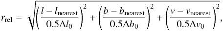 (1)where Δl0, Δb0, Δv0 are dimensions of the bubble (Table 1 in Paper I), coordinates of the outside pixel are l,b,v and coordinates of the inside pixel are lnearest, bnearest, vnearest. As we are dealing only with pixels near the equator, Eq. (1) is precise enough even without the cos(b) correction. We intentionally use the distance towards the nearest pixel of the HI bubble and not the distance towards the centre of the shell, for example. Our choice takes irregular shapes of HI holes into account better. It is also less sensitive to inaccurate measurements of shell dimensions and positions.
The choice of the relative distance has some advantages over using the absolute distances. First, we remove the dependence on units (degrees and km s-1). Second, the difference between angularly different shells is suppressed (the same physical distance between two objects depends on the distance of the observer and by using the ratio between the projected distance and dimensions we take this into account). The same holds for the offset in the LSR velocity.
We are dealing with expanding structures and therefore we cannot convert the lbv-datacube into an xyz-datacube using kinematic distances; it would be too inaccurate or simply wrong. For the whole structures (HI shells, CO clumps) we can calculate the distance and physical dimensions, but for the work with all pixels in the datacube we are limited to the lbv-space and our relative distance.
The value of rrel is >0 for pixels outside HI bubbles.
For pixels inside HI bubbles we calculate the relative distance to the centre of the shell. In Eq. (1), instead of (lnearest, bnearest, vnearest), we take coordinates of the shell centre given in Table 1 of Paper I, and then subtract 1. It makes rrel< 0: pixels close to the wall have rrel close to 0, while those close to the centre of the bubble have rrel close to −1.
According to its relative distance rrel we ascribe each pixel its type:
-
1.
inner bubble: inside one of the HI bubbles with rrel ≤ −0.25
-
2.
outer bubble: inside one of the HI bubbles with 0 >rrel> −0.25
-
3.
inner wall: not part of any HI bubble with 0 <rrel ≤ 0.2
-
4.
outer wall: not part of any HI bubble with 0.2 <rrel ≤ 0.5
-
5.
outside wall: not part of any HI shell with 0.5 <rrel ≤ 1.0
-
6.
far outside: not part of any HI shell with 1.0 <rrel ≤ 2.0
-
7.
unperturbed: not part of any HI shell with rrel> 2.0.
These terms are simply names. These names could be Environment 1, 2, etc., but we believe that our designation is slightly more illustrative. The division between different types was made by looking at profiles of many structures (see below) and by dividing the studied pixels into groups of roughly the same size. The interior (i.e. the bubble) was divided into two parts, inner and outer, to see whether there is any difference in behaviour between parts of the bubble close to walls and further from them. The same holds for walls.
3.3. THI and CO filling factor and the molecularization level
The good way to describe HI in some types of environments (e.g. inside one of the HI bubbles, see the previous section for the list of environments) is the average brightness temperature THI, which is an estimate of the density in the given type of environment. However, for the molecular medium it is not as good because the medium is clumpy and often optically thick, and temperatures in CO clumps are not the straightforward description of densities in the medium. Instead, we calculate the CO filling factor fCO of a region or pixel type as the ratio of a number of pixels with a significant CO temperature to a total number of pixels. “Significant CO temperature” means TCO ≥ TCOcutoff.
The level of molecularization – the ratio of the molecular density to the total density – in a given place/pixel with observed HI and CO temperatures is given by ε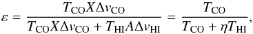 (2)where ΔvCO and ΔvHI are the channel widths of CO and HI datacubes (which are similar, but not the same), X is the famous X factor for which we use the value X = 1.8 × 1020 cm-2 K-1 (km s-1)-1, and A = 1.82 × 1018 cm-2 K-1 (km s-1)-1. The value of η is
 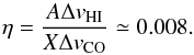 (3)CO is often optically thick and then using the simple relation between the density and brightness (main-beam) temperature underestimates the real density in the environment. In the case of the optically thick medium, ε from Eq. (2) is artificially lower than its real (unknown) value.
By using the CO cutoff temperature, it can be understood that we are interested in the regions where the particle density of the molecular medium forms at least a fraction εsigCO of the total density (Eq. (2)),
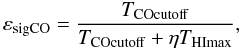 where THImax is the maximum HI temperature (150 K in the LAB survey for the 2nd and 3rd quadrants). Quantified for the TCOcutoff = 0.6 K it means that the molecular medium forms at least one third of the total particle density in the region with a significant CO emission. Translated into masses it says that in such regions at least 2/3 of the mass is molecular.
3.4. Relative profiles
Using rrel from Eq. (1) we calculate the average profiles of THI, fCO, and ε as the average value for a given interval of rrel. We can do it for the whole studied area, i.e. the 2nd and 3rd quadrant, or for each HI shell separately. Using the relative distance rrel has the advantage of scaling the distances of pixels to the dimension of a given shell.
The average profile, composed of profiles of all shells, is dominated by angularly large structures since the relative weight of the shell in the composite picture depends on the amount of pixels the shell contains.
3.5. CO clumps
Another way to describe the CO distribution is to use the natural clumpiness of CO and deal with CO clumps, not with the smooth continuous distribution. We identify clumps in the CO using the DENDROFIND algorithm described by Wünsch et al. (2012).
The clump-finding algorithm DENDROFIND is similar to the well-known CLUMPFIND (Williams et al. 1994), over which it has some advantages, mostly of the technical character. It searches for clumps that 1) are contiguous volumes in the position-position-velocity space; 2) consist of more than a prescribed number of pixels (Npxmin); and 3) where the difference between the clump peak temperature and the temperature at which it borders with the neighbouring clump is higher than a value dTleaf. The clump finding is performed only for pixels with a temperature above a cutoff Tcutoff. The fourth parameter of the DENDROFIND is the number of levels Nlevels into which the temperature scale between the maximum temperature in the analysed datacube and the cutoff temperature Tcutoff is divided; for large values of Nlevels, the results of DENDROFIND cease to depend on it. Overall, results of DENDROFIND do depend on technical parameters (Npxmin, dTleaf, and Tcutoff), but the dependence is predictable and not steep.
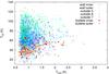 |
Fig. 2 Relation between CO and HI temperatures (Tcl,CO, Tcl,HI) of CO clumps. |
Different environments in the Galaxy: filling factors and CO clump properties.
With the cutoff temperature Tcutoff = TCOcutoff set to 0.6 K, the minimum size of the clump set to Npxmin = 5 and the difference between clumps dTleaf = 0.3 K, DENDROFIND analysis produces 2617 clumps. The number changes slightly when using slightly different values for parameters Npx and dTleaf and changes significantly for different cutoff temperatures TCOcutoff (see Sect. 4).
For further analysis each clump is characterized by coordinates of its centre of mass, its radius, average HI temperature Tcl,HI, its maximum and average CO temperatures Tmax,cl,CO and Tcl,CO, average molecularization εcl, and number of pixels. Radius of a clump is defined as the average distance of pixels belonging to it from its centre. We also calculate the average HI temperature just outside the clump (e.g. from its edge to a distance equal to three times clump radius from its centre) Tcl,HI,out. Figure 2 shows the average HI and CO temperatures for identified clumps.
4. Results
4.1. CO in HI shells
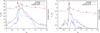 |
Fig. 3 Average HI temperature (left) and CO filling factor (right) as a function of the relative distance rrel. Black solid line shows the average for the whole datacube, blue solid line shows the profile for one Galactic HI supershell, GS242-03+37. Dotted lines show the number of pixels, from which the average was calculated. Red lines with numbers give extents of different “types of environment”. Red arrows indicate the transition between bubbles and walls. |
Table 1 shows the type of the environment (first column) and its fraction qlbv in the complete datacube (second column). Numbers label pixels of different environments: 1 and 2 inside bubbles; 3 and 4 inside walls; 5, 6, and 7 outside shells; 0 for all environments (see Methods for a more detailed explanation). The average HI temperatures THI are in the third column; the fourth column shows the CO filling factors fCO (in %), which tell how much space of the environment is occupied by regions with a significant CO emission, i.e. TCO ≥ 0.6 K, which is the same value as that used in DENDROFIND for the clump identification. The fifth, sixth, and seventh columns give average results for regions with significant CO emission only, i.e. inside CO clumps: the average HI and CO temperatures, and molecularization (TCOsig,HI, TCOsig,CO, ε).
Bubbles themselves fill only a small fraction of the studied volume, walls occupy a much larger space. This is a consequence of several factors: first, some of the HI shells are not contained (or not completely contained) in the studied datacubes, but their walls are there. Furthermore, shapes of HI shells are not ideal/smooth/spherical and all higher density protrusions or even embedded structures with higher THI count as walls in the searching mechanism.
Results in Table 1 depend on several quantities. The most important is the catalogue of shells, more precisely, their precise identification, as it gives the distribution of studied pixels into “environments” (Col. 1). Then the results depend on cutoffs, especially on the CO cutoff (e.g. different values of the limit for the significant CO emission lead to different values of fCO), but also on the HI cutoff (though only mildly). However, the trends we observe, for example the dependence of ε on the environment, are the same.
Figure 3 shows the average profile of the THI and fCO as a function of the relative distance rrel. It is the average of the whole datacube. Since HI bubbles were identified as local minima, it is not surprising that the average HI temperature is low inside them, with the HI temperature in the inner bubble (environment 1) being lower than in the outer bubble (environment 2). Maximum values are reached in walls, especially in outer walls (environment 4), with the distance (1.2−1.5)rrel from the centre of the shell (or (0.2−0.5)rrel from the transition bubble-wall). All these values have high dispersion and depend on the local conditions and on the position in the Galaxy. Figure 3 also shows the relative profile of one individual shell. It is the Galactic supershell GS242-03+37, one of the largest shells in the outer Milky Way and a very pronounced one. It was first identified by Heiles (1979).
How much of the space is occupied by the CO emission with (TCO ≥ 0.6 K)? The largest amount of CO is found in the inner walls of HI shells, more than in the outer wall, even though it is still quite a high value. A high value of fCO is also found in the outer bubble environment, close to the wall. It seems that CO is more concentrated than HI towards the inner wall of the HI shell or towards the transition bubble-inner wall.
The CO emission is always associated with high (or higher) HI temperatures, as seen in the fifth column of Table 1. These values are not simply correlated to the average HI temperature in the environment. The average CO temperatures in regions with significant CO emission (as given in the sixth column) are slightly higher in bubbles than in walls. The molecularization behaves the other way round: ε is higher inside bubbles than in walls.
 |
Fig. 4 Number of CO clumps as a function of their relative distance TCO. |
4.2. CO clumps relative to HI shells
For the centre of each CO clump we find the relative distance rrel to its nearest bubble using Eq. (1) and then calculate the distribution of CO clumps as a function of rrel: ncl(rrel). Since the different rrel are contained differently in the studied datacube, we compute the relative frequency of pixels with rrel in certain interval of values: qrrel(rrel). With it we derive the normalized frequency of clumps ncl,norm(rrel):  (4)Figure 4 shows the distribution of ncl(rrel), f(rrel), and ncl,norm(rrel). The function ncl,norm(rrel) has a sharp maximum at rrel = 0.0 corresponding to walls of HI shells or, more precisely, to the transition between the low-density outer bubbles and high-density inner walls of HI shells.
Table 2 shows average properties of CO clumps in different media. Though the trends seen in Table 2 are the same as in Table 1, the numbers are slightly different because now the average is done in two steps, first for each clump and then for all clumps, not in one step for all pixels as was done previously. Basically, in the first approach – Table 1 – all pixels have the same weight, while in the second approach – Table 2 – the weight depends inversely on the size of the clump to which the pixel belongs. Table 2, similarly to Table 1, depends on the temperature cutoffs, but again, trends indicated in this Table are not dependent on its precise value: the change from 0.3 K to 0.6 K does not give different results.
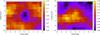 |
Fig. 5 Fraction of CO clumps falling into the interiors of HI shells (left) or into their walls (right) as a function of the artificial offset of CO clumps positions in l and v. Zero offsets correspond to the “real situation”, non-zero offsets test the robustness of the relation between HI shells and CO clumps. |
Average properties of CO clumps based on their position towards HI shells.
To test if the distribution of CO clumps in a relation to HI shells is random or not, we artificially shift positions of CO clumps by an offset in the l, b, or v direction and then look at the number of clumps that fall to the bubbles (i.e. interiors of HI shells – environments 1 and 2) and to the walls (environments 3 and 4). Offsets are mutually independent and are the same for all clumps. Results are shown in Fig. 5. We only show calculations with l and v offsets, since the b offsets can only be small (our datacube is quite narrow in the b-direction). The left panel of Fig. 5 shows the ratio between the number of CO clumps falling into the interiors of HI shells and the total number of clumps as a function of the offset in l and v. This ratio has a clear minimum for the zero offsets, corresponding to the “real situation”. The right panel of Fig. 5 shows the fraction of CO clumps falling into walls of HI shells. The largest values of this ratio are for the smallest offsets. These results show that CO clumps are not distributed randomly, but rather in such a way that interiors of HI shells contain very few CO clumps, while walls contain a lot of them.
4.3. Close environment of CO clumps
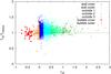 |
Fig. 6 Ratio of the inside and outside HI temperatures for CO clumps as a function of the relative distance rrel. |
For each CO clump we calculate the ratio of the average HI temperatures inside Tcl,HI and outside of it Tcl,HIout (for the calculation we used the outside as three times larger than the size of the clump, but results are similar for other values). In Fig. 6 we see that the spread in values is high, but that the clumps inside bubbles tend to have the ratio between inside and outside HI temperatures close to 1, while other clumps (dominated by wall clumps) tend to have a slightly higher value of 1.1 (see average values in Table 2). Their dispersion seems to be much higher, but since the number of bubble clumps is small, we do not quantify it.
4.4. Which HI shells support or inhibit CO creation
We tried to find a correlation between properties of HI shells and a number of associated clumps. Unfortunately, we are very much bound by the relatively low resolution of observations. We found that the larger the angular size of the shell or its velocity extent is, the more clumps it is associated with, which is obviously an effect of the resolution. The other correlation we found is that the larger galactocentric distance of the HI shell (computed as the kinematic distance using shell radial velocity and the rotation curve of the Milky Way, see Paper I) means fewer associated CO clumps, which is also not surprising.
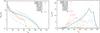 |
Fig. 7 Frequency of different HI temperatures (left) and the CO filling factor (right) as a function of the HI temperature. |
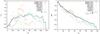 |
Fig. 8 Average CO temperature (left) and the molecularization (right) as a function of the HI temperature. |
5. Discussion
5.1. Rearrangement, destruction and creation of CO clumps
There is a real lack of CO clumps inside HI shells. And those that are inside have properties different from those in walls. Therefore, we assume that some of the preexisting CO clumps were destroyed by the activity that created HI shells; a part survived, but their diffuse component (mostly HI) was removed; and a part was shifted to walls, away from the destructive forces.
We find quite a strong evidence that preexisting CO clumps inside HI shells were changed: lower Tcl,HI , larger Tcl,CO, larger fCO, lower Tcl,HI/Tcl,HIout. The removal of the diffuse component (HI and partly CO) seems to be a good explanation of these observations. What we do not know is what fraction of preexisting clumps was destroyed and what fraction was moved to the walls. Looking at Fig. 7 we are inclined to say, that the inner wall contains a significant amount of pushed and robbed CO clumps, apart from newly created or preexisting mostly uninfluenced CO clumps, while the outer wall contains mainly the latter type of clumps. The HI temperature distribution (DFHI) is similar for both walls, but the dependence of the CO filling factor fCO on the HI temperature differs and for the inner wall it looks like an intermediate stage between the profile for bubble CO clumps and outer wall clumps.
It is easier to calculate the total outcome of these two conflicting effects, the destruction of preexisting clumps, and creation of new ones. We assume that the environment outside (5, 6, and 7 in the tables) accurately describes conditions that are not influenced by the presence of HI shells. Then, using the values in Table 2 we calculate that the total number of CO clumps in the studied region should be 1038. That is 2.5 times smaller than the measured value (which is 2617).
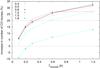 |
Fig. 9 Estimated increase in the number of CO clumps as a function of CO and HI cutoffs. The x-axis gives the HI cutoff, the y-axis shows the percent increase in the number of clumps. Different lines shows different CO cutoffs (cutoff values are shown in K). |
This is slightly unfair towards the outside since this environment contains a lot of low-density (i.e. low HI temperature) gas, and the amount of CO depends on the density of ambient gas. If we restrict ourselves to the environment “outside 5”, which has a similar HI temperature distribution as both walls (inner and outer) – see DFHI at Fig. 7 – and take these values as typical of the unperturbed medium, we come to the expected total number of CO clumps of 2210. The real value is larger by about 20%.
The derived increase in the number of CO clumps depends on values in Tables 1 and 2, which depend on temperature cutoffs TCOcutoff and THIcutoff. Figure 9 shows the percent increase in the number of CO clumps as a function of these cutoffs. As canonical values we use THIcutoff = 0.3 K, corresponding to three times the rms noise in the data, and TCOcutoff = 0.6 K, as explained in Sect. 2. The percent increase is shown, as the number of CO clumps depends very strongly on the TCOcutoff temperature, ranging from ~3700 for TCOcutoff = 0.4 K, through ~2600 for TCOcutoff = 0.6 K, to ~1000 for TCOcutoff = 1.5 K. In Fig. 9 we see that for CO cutoffs below ~1.5 K, the increase is nearly independent of the value of the CO cutoff. Above 1.5 K, results substantially change, but then, values above 1.5 K are probably too high to be used as a threshold. It is nonetheless interesting to see the difference in the behaviour of lower and higher density (corresponding to lower and higher brightness temperature) molecular gas in connection to HI shells.
The increase in the number of CO clumps also depends on the HI cutoff. For reasonable values of this THIcutoff, i.e. well above the rms noise in the HI data (0.09 K) and not too much above it, the resulting increase lies in the range between 15 and 25%.
This 20% increase in the number of CO clumps is the net outcome where destroyed CO clumps are deducted from newly created CO clumps. It is a very rough estimate, but it seems that after all, HI shells (and more precisely, energetic activities that create HI shells) have on average a positive outcome on the amount of CO in the Galaxy.
5.2. Reliability of results
Our results are, obviously, dependent on what we consider to be HI shells and this is a source of two types of errors:
-
Problem 1: the dimensions of the shells are wrong (under- or overestimated);
-
Problem 2: an HI shell is not real, i.e. the identification is false.
We deal with these problems separately. Owing to our way of calculating the relative distance to the nearest pixel of the bubble, and to our clean separation of bubble and other pixels, Problem 1 is not so serious. It leads to slightly incorrect relative distances. Pixels close to the interesting bubble/wall frontier are not influenced so much. This problem leads to “smearing” in observed behaviour, but not to different trends.
Problem 2 is more serious and its influence cannot be so easily estimated. In this paper we take as a basis for our analysis the catalogue of HI shells from Paper I. This catalogue – like other catalogues of HI shells – probably contains some false identifications and probably misses some real structures as well. We discuss the different identifications in Paper I where a comparison between different catalogues of HI shells is provided. A similar comparison is given in Suad et al. (2014), which is also a catalogue of HI shells in the outer Milky Way, based on the LAB HI survey, but using a very different identification technique. Our identification technique is based on locating HI holes, while theirs is based on locating HI walls. In an ideal case these two approaches should find the same objects, but we can easily imagine (and find in datacubes) structures that do not have easily identifiable walls or, on the other hand, structures that are formed mostly by fragmented walls.
The main result of the comparison in Suad et al. (2014) is that there are shells that are found in only one of these catalogues: Suad’s catalogue contains about twice as many shells as ours since they also include open structures, but they reidentify slightly less than half of our structures. More recently, Sallmen et al. (2015) give a comparison of shell catalogues based on observations with different angular resolutions.
To understand if and how much we can trust results based on properties of shells in our catalogue, when we know that our catalogue is not perfect, we constructed a toy model: it consists of Ntot cubes, the cube can be either empty (i.e. filled by the unperturbed medium) or contain the shell (i.e. bubble and wall). Each of these environments (unperturbed, bubble, and wall) has the value of a hypothetical quantity q.
Now, we assume that by using an identification algorithm some of these existing structures are identified as structures (their number is Ndetected), but some are missed (Nmissed). On the other hand, some empty cubes are falsely identified as structures (Nfalse). With these identifications containing errors we calculate observed values of q and compare them to real values and look, how much they are changed by missing and false identifications.
To mimic an analysis we performed in this paper, we define the values of the quantity q as follows: in the unperturbed medium qunperturbed = 1.0, in the walls qwall = 2.0, and inside the bubble qbubble = 0.0. Then, we derive observed values of q from our identifications with errors. If qobs,wall ≥ 1.5 and qobs,bubble ≤ 0.5, we consider the experiment successful, otherwise it is considered marred by incorrect identifications. Filling factors of bubble and wall environments were chosen to resemble those in Table 1, but they were found not to influence following results.
We define the “badness” of the experiment as  (5)and porosity as
  (6)and we found, that the experiment is successful, if
 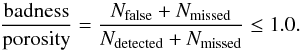 (7)Observed values of qobs,unperturbed usually differed from the input value qunperturbed, but for successful experiments it was always in between qobs,bub<qobs,unperturbed<qobs,wall. It does not depend on some simple criterion like condition (7).
In the case of nearly no missed structures condition (7) leads to Nfalse/Ndetected ≤ 1.0, i.e. to a quite reassuring condition that if at least half of the structures in the catalogue are real, then we might get good enough results. Taking values Nfalse ~ 0.5Ndetected and Nmissed ~ Ndetected (which are based on the comparison of catalogues in Suad et al. 2014) as typical values for our HI shells catalogue (and perhaps any catalogue), we get from Eq. (7) the result badness/porosity ~0.5, which means success, i.e. that the observed trends are real.
Our toy model is certainly very simple, but at least we can tell that our analysis in this paper might detect real trends in the Galaxy, even though there are imperfections in our input data, especially in the catalogue of HI shells.
6. Summary
The distribution of CO clumps is correlated with HI shells: the interiors of bubbles are devoid of both HI and CO. CO clumps tend to sit in the walls of HI shells (Fig. 3), they are concentrated in the region between low HI temperature bubbles and high HI temperature walls of the shells. CO is more concentrated than HI to the bubble/wall transitions. HI walls are much thicker; the typical thickness is ~0.5rrel.
The increased molecularization in bubble CO clumps is mostly given by the lower values of HI temperatures (as a consequence of Eq. (2)), though it might be slightly increased compared to wall CO clumps, as seen in Fig. 8.
The HI environment of bubble CO clumps seems to be rather flat. There is no increase in HI inside the clumps and there are no big changes outside it (see Fig. 6 for the value and dispersion of the ratio inside and outside HI temperature). Actually, not even wall CO clumps coincide with the HI maxima (they probably coincide with past HI maxima), but the region around them is typically more diverse and less flat than around bubble CO clumps.
CO clumps inside bubbles have relatively low HI temperatures compared to CO clumps in walls or outside – it is nicely seen in Fig. 2 – but for this lower HI temperature they tend to have larger CO filling factor fCO (see Fig. 7).
7. Conclusions
Based on our analysis of HI shells in the outer Milky Way, we draw the following conclusions:
-
In interiors of HI shells and in regions of the decreased HI density, CO clumps are smaller and contain less HI than clumps in walls of HI shells or clumps outside HI shells. It seems that some CO clumps inside these bubbles were destroyed and the remaining ones were robbed of their more diffuse gas.
-
A substantial amount of CO clouds exist outside HI shells. They are often quite massive and tend to have a large HI content. They are probably formed independently of HI shells.
-
In walls of HI shells there is an increased occurrence of CO clumps. This increase cannot be simply explained by the higher HI densities and looking at differences between clumps in walls and in an unperturbed medium outside of HI shells, we estimate the total increase of CO in the outer Milky Way due to HI shells being around 20%.
Acknowledgments
This study has been supported by the Czech Science Foundation grant 209/12/1795, the MŠMT grant LG14013 and by the project RVO: 67985815. The authors would like to thank the anonymous referee for constructive comments leading to the improvement of the paper.
References
- Anderson, L. D., Zavagno, A., Deharveng, L., et al. 2012, A&A, 542, A10 [NASA ADS] [CrossRef] [EDP Sciences] [Google Scholar]
- Bagetakos, I., Brinks, E., Walter, F., et al. 2011, AJ, 141, 23 [NASA ADS] [CrossRef] [Google Scholar]
- Bureau, M., & Carignan, C. 2002, AJ, 123, 1316 [NASA ADS] [CrossRef] [Google Scholar]
- Churchwell, E., Povich, M. S., Allen, D., et al. 2006, ApJ, 649, 759 [NASA ADS] [CrossRef] [Google Scholar]
- Dame, T. M., Hartmann, D., & Thaddeus, P. 2001, ApJ, 547, 792 [NASA ADS] [CrossRef] [Google Scholar]
- Dawson, J. R., McClure-Griffiths, N. M., Kawamura, A., et al. 2011, ApJ, 728, 127 [NASA ADS] [CrossRef] [Google Scholar]
- Dawson, J. R., McClure-Griffiths, N. M., Wong, T., et al. 2013, ApJ, 763, 56 [NASA ADS] [CrossRef] [Google Scholar]
- Deharveng, L., Schuller, F., Anderson, L. D., et al. 2010, A&A, 523, A6 [NASA ADS] [CrossRef] [EDP Sciences] [Google Scholar]
- Ehlerová, S., & Palouš, J. 2005, A&A, 437, 101 [NASA ADS] [CrossRef] [EDP Sciences] [Google Scholar]
- Ehlerová, S., & Palouš, J. 2013, A&A, 550, A23 (Paper I) [NASA ADS] [CrossRef] [EDP Sciences] [Google Scholar]
- Heiles, C. 1979, ApJ, 229, 533 [NASA ADS] [CrossRef] [Google Scholar]
- Kalberla, P. M. W., Burton, W. B., Hartmann, D., et al. 2005, A&A, 440, 775 [NASA ADS] [CrossRef] [EDP Sciences] [Google Scholar]
- McClure-Griffiths, N. M., Dickey, J. M., Gaensler, B. M., & Green, A. J. 2002, ApJ, 578, 176 [NASA ADS] [CrossRef] [Google Scholar]
- Mizuno, D. R., Kraemer, K. E., Flagey, N., et al. 2010, AJ, 139, 1542 [NASA ADS] [CrossRef] [Google Scholar]
- Ott, J., Walter, F., Brinks, E., et al. 2001, AJ, 122, 3070 [NASA ADS] [CrossRef] [Google Scholar]
- Rhode, K. L., Salzer, J. J., Westpfahl, D. J., & Radice, L. A. 1999, AJ, 118, 323 [NASA ADS] [CrossRef] [Google Scholar]
- Sallmen, S. M., Korpela, E. J., Bellehumeur, B., et al. 2015, AJ, 149, 189 [NASA ADS] [CrossRef] [Google Scholar]
- Sidorin, V., Douglas, K. A., Palouš, J., Wünsch, R., & Ehlerová, S. 2014, A&A, 565, A6 [NASA ADS] [CrossRef] [EDP Sciences] [Google Scholar]
- Simpson, R. J., Povich, M. S., Kendrew, S., et al. 2012, MNRAS, 424, 2442 [NASA ADS] [CrossRef] [Google Scholar]
- Stewart, S. G., Fanelli, M. N., Byrd, G. G., et al. 2000, ApJ, 529, 201 [NASA ADS] [CrossRef] [Google Scholar]
- Suad, L. A., Caiafa, C. F., Arnal, E. M., & Cichowolski, S. 2014, A&A, 564, A116 [NASA ADS] [CrossRef] [EDP Sciences] [Google Scholar]
- Tenorio-Tagle, G., & Bodenheimer, P. 1988, ARA&A, 26, 145 [NASA ADS] [CrossRef] [Google Scholar]
- Tenorio-Tagle, G., Franco, J., Bodenheimer, P., & Rozyczka, M. 1987, A&A, 179, 219 [NASA ADS] [Google Scholar]
- van Eymeren, J., Marcelin, M., Koribalski, B., et al. 2009, A&A, 493, 511 [NASA ADS] [CrossRef] [EDP Sciences] [Google Scholar]
- Walch, S., Whitworth, A. P., Bisbas, T. G., Hubber, D. A., & Wünsch, R. 2015, MNRAS, 452, 2794 [NASA ADS] [CrossRef] [Google Scholar]
- Wünsch, R., Jáchym, P., Sidorin, V., et al. 2012, A&A, 539, A116 [NASA ADS] [CrossRef] [EDP Sciences] [Google Scholar]
All Tables
All Figures
|
Fig. 1 Galactic longitude-velocity map at the Galactic latitude b = 0° of the outer Milky Way: HI (map), CO (green contours) and HI shells (blue outlines). |
| In the text | |
|
Fig. 2 Relation between CO and HI temperatures (Tcl,CO, Tcl,HI) of CO clumps. |
| In the text | |
|
Fig. 3 Average HI temperature (left) and CO filling factor (right) as a function of the relative distance rrel. Black solid line shows the average for the whole datacube, blue solid line shows the profile for one Galactic HI supershell, GS242-03+37. Dotted lines show the number of pixels, from which the average was calculated. Red lines with numbers give extents of different “types of environment”. Red arrows indicate the transition between bubbles and walls. |
| In the text | |
|
Fig. 4 Number of CO clumps as a function of their relative distance TCO. |
| In the text | |
|
Fig. 5 Fraction of CO clumps falling into the interiors of HI shells (left) or into their walls (right) as a function of the artificial offset of CO clumps positions in l and v. Zero offsets correspond to the “real situation”, non-zero offsets test the robustness of the relation between HI shells and CO clumps. |
| In the text | |
|
Fig. 6 Ratio of the inside and outside HI temperatures for CO clumps as a function of the relative distance rrel. |
| In the text | |
|
Fig. 7 Frequency of different HI temperatures (left) and the CO filling factor (right) as a function of the HI temperature. |
| In the text | |
|
Fig. 8 Average CO temperature (left) and the molecularization (right) as a function of the HI temperature. |
| In the text | |
|
Fig. 9 Estimated increase in the number of CO clumps as a function of CO and HI cutoffs. The x-axis gives the HI cutoff, the y-axis shows the percent increase in the number of clumps. Different lines shows different CO cutoffs (cutoff values are shown in K). |
| In the text | |
Current usage metrics show cumulative count of Article Views (full-text article views including HTML views, PDF and ePub downloads, according to the available data) and Abstracts Views on Vision4Press platform.
Data correspond to usage on the plateform after 2015. The current usage metrics is available 48-96 hours after online publication and is updated daily on week days.
Initial download of the metrics may take a while.