| Issue |
A&A
Volume 586, February 2016
|
|
|---|---|---|
| Article Number | A56 | |
| Number of page(s) | 5 | |
| Section | Stellar structure and evolution | |
| DOI | https://doi.org/10.1051/0004-6361/201527609 | |
| Published online | 27 January 2016 | |
Research Note
Time properties of the the ρ-class burst of the microquasar GRS 1915+105 observed with BeppoSAX in April 1999
1 INAF, IASF Palermo, via U. La Malfa 153, 90146 Palermo, Italy
e-mail: This email address is being protected from spambots. You need JavaScript enabled to view it.
2 INFN, Sezione Roma 1, Piazzale A. Moro 2, 00185 Roma, Italy
3 INAF, IAPS, via del Fosso del Cavaliere 100, 00113 Roma, Italy
4 In Unam Sapientiam, Piazzale A. Moro 2, 00185 Roma, Italy
Received: 21 October 2015
Accepted: 15 December 2015
Abstract
We present a temporal analysis of a BeppoSAX observation of GRS 1915+105 performed on April 13, 1999 when the source was in the ρ class, which is characterised by quasi-regular bursting activity. The aim of the present work is to confirm and extend the validity of the results obtained with a BeppoSAX observation performed on October 2000 on the recurrence time of the burst and on the hard X-ray delay. We divided the entire data set into several series, each corresponding to a satellite orbit, and performed the Fourier and wavelet analysis and the limit cycle mapping technique using the count rate and the average energy as independent variables. We found that the count rates correlate with the recurrence time of bursts and with hard X-ray delay, confirming the results previously obtained. In this observation, however, the recurrence times are distributed along two parallel branches with a constant difference of 5.2 ± 0.5 s.
Key words: binaries: close / X-rays: stars
Retired.
© ESO, 2016
1. Introduction
The bursting behaviour (see the review paper by Fender & Belloni 2004) characterises the ρ class of GRS 1915+105 X-ray emission (Belloni et al. 2000). It was discovered in 1996 with Rossi-XTE (Taam et al. 1997) and interpreted as the result of instabilities in an accretion disk, as expected by some previous theoretical calculations (Taam & Lin 1984). This particular behaviour of GRS 1915+105, known in the literature as heartbeat, exhibits the properties of a limit cycle (e.g. Szuszkiewicz & Miller 1998; Janiuk & Czerny 2005) that has been extensively studied under many aspects (see, for instance, Neilsen et al. 2011, 2012). The discovery of a similar phenomenon in IGR J17091−3624 (Altamirano et al. 2011) and MXB 1730-335 (Rapid Burster, Bagnoli & in’t Zand 2015) makes the interest in these studies more general, and comparative analyses can be useful to obtain a more complete picture of the physics underlying these cycles.
Observation log of the 1999 observation: ObsId 20985001.
In some previous papers (Massaro et al. 2010; Mineo et al. 2012; Massa et al. 2013, hereafter Papers I, II, and III, respectively), we investigated the properties of the burst series emitted by the micro-quasar GRS 1915+105 in the ρ class. In particular, using the data of a long BeppoSAX observation performed in October 2000, we reported several interesting correlations between the mean burst recurrence time Trec and the X-ray photon count rate. We developed a method for measuring the hard X-ray delay (HXD) based on the loop trajectories described in the count rate – mean photon energy (CR-E) plane during the bursts (Paper III). We found that HXD, which basically is the time separation between the midpoints of the count rate and mean photon energy curves of each burst (see Sect. 3.2), is related to the brightness level of the source. The aim of the present analysis is to confirm and extend the validity of our previous results with different independent data and to explore to which extent these correlations are stable. We considered another observation of BeppoSAX, performed in April 1999, whose analysis has never been published. We applied the same methods as used in the previous studies, which we do not describe here for the sake of brevity.
2. Observation and data reduction
We analysed the BeppoSAX observation of GRS 1915+105 performed on April 13, 1999. We used data obtained with the Medium Energy Concentrator Spectrometer (MECS) in the 1.6–10 keV energy band (Boella et al. 1997), which were retrieved from the BeppoSAX archive at the ASI Science Data Center (ASDC). Data were reduced and selected following the standard procedure and using the SAXDAS v. 2.3.3 package. MECS events were selected within a circle of 8′ radius that contains about 95% of the point source signal. No background was considered because the source rate is two orders of magnitude higher than the contemporary background level evaluated in a region far from the source. Its subtraction is then irrelevant in the analysis.
We divided the entire data set into several series, each corresponding to a satellite orbit, and named them according to the same criterion as adopted in Paper I for the 2000 data. Each series corresponds to a continuous observing period and is tagged with the letter P followed by the orbit sequential number; if a particular series is interrupted because of telemetry gaps, a letter is added to the series’ numbers. The analysis is performed over segments with exposures longer than 1000 s to have sufficient statistics. Table 1 lists the codes of the considered 18 series, the starting times, the exposure lengths, the number of bursts, and other quantities derived from our analysis.
3. Data analysis and results of the 1999 ρ-class observation
The temporal analysis of data in ρ mode, performed taking into account the results presented in Papers I and III, was focused on evaluating the recurrence time of the bursts and of the HXD.
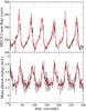 |
Fig. 1 Time evolution of the series P3b. The top panel shows a short portion of the light curve in the entire MECS energy range; the bottom panel presents the relative mean energy. Black curves are the rates with 1 s integration time, while red curves are averaged in a 5 s interval. |
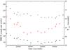 |
Fig. 2 Time evolution (left scale) of the average burst (open black circle) and mean BL (black circle) count rate and of Trec of bursts (red points, right scale) during the observation in April 1999. |
3.1. Recurrence time of bursts
All data series present regular sequences of bursts typical of the ρ class, characterised by a slow leading trail (SLT), a pulse, and a final decaying trail (FDT; see Paper I) superposed onto a baseline level (BL) that remains remarkably constant in each series. The BL rate was evaluated in the three seconds after the minimum between two consecutive bursts. A 300 s long segment of the series P3b is shown in the upper panel of Fig. 1.
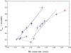 |
Fig. 3 Trec vs. the BL rate during the April 1999 observation. The dot-dashed blue lines are the linear best fits to the data of the two branches with the same slope. The initial point is marked by a red circle. The dotted lines connecting the points describe the time sequence of data. |
A small but significant variation of the total brightness with a relative amplitude of ~18%, from a mean count rate of 232.4 ct/s at the beginning of the observation to 196.6 ct/s in the middle, is clearly visible (see Fig. 2). A similar trend is also detected in the BL light curve, but with higher amplitude (~27%). We note that the dynamical range of the observed variability remains within the range detected in October 2000 (see Paper I).
As in Paper I, we evaluated the recurrence time of bursts by means of Fourier power spectra of each series. These periodograms generally presented a single sharp dominant peak (S type, according to the definition given in Massaro et al. 2010) with the exception of only two series that presented two peaks (T type) with a quite small separation (see Table 1). The values of Trec, also given in Table 1, follow the same trend as the count rate, as shown in Fig. 2, in agreement with our findings in the October 2000 observation. We note, however, that its variation (~26%) has an amplitude that is almost identical to those of the BL rate.
The plot in Fig. 3 shows the relation between Trec and the BL count rate starting from the first series marked by a red point. It is interesting to note that points are located in two clearly separated branches: the lower branch corresponds to the initial decreasing rate time interval, and the upper branch occurred during the subsequent increasing source count rate. No effect like this was detected in the observation of October 2000 because the count rate never decreased (Paper I).
To quantify the systematic difference in Trec between the two branches, we computed the linear fits to the data (excluding the first point) and obtained similar values for the slopes; we then fixed both values to the mean value. The constant difference between the two lines (see Fig. 3) is 5.2 ± 0.5 s, about 11% of the mean Trec in the pointing.
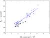 |
Fig. 4 Comparison of the Trec vs. BL count rate between observations made in April 1999 (black filled circles) and October 2000 (blue diamonds). |
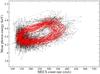 |
Fig. 5 Trajectory in the CR-E plane for 1 s integration time (black curve) and 5 s integration time (red curve). |
We found that Trec is proportional to the third power of the BL count rate, as shown in Fig. 4. For comparison, the values relative to the October 2000 observation are also plotted in the same figure: the upper branch of the 1999 data agrees well with the 2000 data, while the decreasing branch lies systematically below these points. When we fitted all data (1999 and 2000) with a power law, we obtained an exponent equal to 3.1 ± 0.1.
3.2. Mapping in the CR-E plane and the HXD
Applying the same approach as described in Paper III, we computed the data series of the mean photon energy (see the lower panel in Fig. 1), which were used to construct the curves in the CR-E plane. Again we found that each series describes a well-defined loop of approximately elliptical shape. An example that is useful for illustrating the limit cycle typical of the ρ class is given in Fig. 5 for the P3b data; the other series exhibit very similar trajectories. The structure of the limit cycle is related to a delay between the count rate (photon luminosity) and the mean photon energy (temperature) curves. This delay of high-energy photons is clearly apparent from the mean burst shape and energy curve plotted in Fig. 6 for the two data series P3b (black curves) and P16 (red curves), which correspond to points in the decreasing and increasing branch that have similar BL rates but average Trec equal to 46.0 s and 51.9 s, respectively. We computed these mean curves by means of the algorithm applied to the CR-E trajectories; this is explained in detail in Massaro et al. (2014).
The definition of HXD used in our works (see Paper III) is graphically explained in Fig. 6 with the vertical lines: it measures the time separation between the corresponding midpoints of the two curves for each bursts. The resulting mean values HXD for each series are also given in Table 1: similar as for the 2000 data, a positive correlation between the delay and Trec was found, as shown in Fig. 7, where a two-branch path is also clearly apparent.
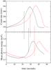 |
Fig. 6 Comparison between the average burst profiles (top panel) in the series P3b (black) and P16b (red) and between the relative mean energies (bottom panel). Vertical lines show how HXD is measured from the midpoints times of the two data series. |
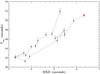 |
Fig. 7 Trec vs. HXD the during the April 1999 observation. The initial point is marked by the red circle. The dotted lines connecting the points describe the temporal evolution of data. |
In Paper III we found that HXD is proportional to the third power of the BL count rate; a relation similar to that of Trec. We verified that the correlation between HXD and the cube of the BL rates also holds for these data.
4. Summary and conclusion
We analysed a BeppoSAX observation of GRS 1915+105 performed in April 1999 when it was in the ρ-variability class and compared the results with those of another previously studied longer pointing of October 2000. The main properties of the ρ class were confirmed: the positive correlation between the recurrence time of bursts and the BL rate, the closed trajectories in the CR-E plane, and the occurrence of an HXD that was also correlated with both Trec and rate. In this observation, however, the recurrence times Trec are distributed along two parallel branches with a constant difference of 5.2 ± 0.5 s. The peaks’ structure does not show any significant change between the two branches, as clearly apparent in Fig. 8, where two segments of the series P5a and P15 are plotted.
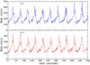 |
Fig. 8 Segments of the 1–6–10 keV series P5a (top panel) and P15 (bottom panel) in the decreasing and increasing branch, respectively. No change of the burst structure is apparent. |
A physical explanation for this double branch effect is unclear, as is the mechanism producing the class bursting. Taam et al. (1997) proposed for the first time that the bursting originates from a non-linear thermal-viscous instability in the accretion disk. However, a dynamical approach to reproduce the observed general structures has not been developed so far. In a first attempt, Massaro et al. (2014) applied the well-known FitzHugh-Nagumo dynamical equations in two non-dimensional variables x and y, which was found to be proportional to the photon flux and disk temperature, respectively. Their time evolution is given by two differential equations, one of which contains a “cooling” term in x3, which is necessary to achieve an unstable equilibrium point around which a limit cycle can be established: 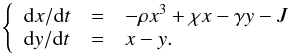 (1)These equations have four parameters, one of which is a forcing J that Massaro et al. (2014) proposed to be related to the mass accretion rate in the disk. They demonstrated that changes of its value affect both the recurrence time of the bursts and the mean level of intensity. Moreover, a change of the same parameter can also move the system to a stable equilibrium point with a transition to a non-bursting behaviour, for example, as observed in the χ class (Belloni et al. 2000). The present finding of the two branches of the Trec-BL rate plot shown in Fig. 7 suggests that in addition to J, at least one of the other structural parameters, for instance χ or γ, should be considered as variable in the burst modelling. A further development of this mathematical model and the physical interpretation of these changes is beyond the goals of this article, however.
Acknowledgments
The authors thank the anonymous referee for improving the paper with constructive comments and suggestions. They also thank the personnel of ASI Science Data Center, particularly M. Capalbi, for help in retrieving BeppoSAX archive data.
References
- Altamirano, D., Belloni, T., Linares, M., et al. 2011, ApJ, 742, L17 [NASA ADS] [CrossRef] [Google Scholar]
- Bagnoli, T., & in’t Zand, J. J. M. 2015, MNRAS, 450, L52 [NASA ADS] [CrossRef] [Google Scholar]
- Belloni, T., Klein-Wolt, M., Méndez, M., van der Klis, M., & van Paradijs, J. 2000, A&A, 355, 271 [NASA ADS] [Google Scholar]
- Boella, G., Chiappetti, L., Conti, G., et al. 1997, A&AS, 122, 327 [NASA ADS] [CrossRef] [EDP Sciences] [Google Scholar]
- Fender, R., & Belloni, T. 2004, ARA&A, 42, 317 [NASA ADS] [CrossRef] [Google Scholar]
- Janiuk, A., & Czerny, B. 2005, MNRAS, 356, 205 [NASA ADS] [CrossRef] [Google Scholar]
- Massa, F., Massaro, E., Mineo, T., et al. 2013, A&A, 556, A84 [NASA ADS] [CrossRef] [EDP Sciences] [Google Scholar]
- Massaro, E., Ventura, G., Massa, F., et al. 2010, A&A, 513, A21 [NASA ADS] [CrossRef] [EDP Sciences] [Google Scholar]
- Massaro, E., Ardito, A., Ricciardi, P., et al. 2014, Ap&SS, 352, 699 [NASA ADS] [CrossRef] [Google Scholar]
- Mineo, T., Massaro, E., D’Ai, A., et al. 2012, A&A, 537, A18 [NASA ADS] [CrossRef] [EDP Sciences] [Google Scholar]
- Neilsen, J., Remillard, R. A., & Lee, J. C. 2011, ApJ, 737, 69 [NASA ADS] [CrossRef] [Google Scholar]
- Neilsen, J., Remillard, R. A., & Lee, J. C. 2012, ApJ, 750, 71 [NASA ADS] [CrossRef] [Google Scholar]
- Szuszkiewicz, E., & Miller, J. C. 1998, MNRAS, 298, 888 [NASA ADS] [CrossRef] [Google Scholar]
- Taam, R. E., & Lin, D. N. C. 1984, ApJ, 287, 761 [NASA ADS] [CrossRef] [Google Scholar]
- Taam, R. E., Chen, X., & Swank, J. H. 1997, ApJ, 485, L83 [NASA ADS] [CrossRef] [Google Scholar]
All Tables
All Figures
|
Fig. 1 Time evolution of the series P3b. The top panel shows a short portion of the light curve in the entire MECS energy range; the bottom panel presents the relative mean energy. Black curves are the rates with 1 s integration time, while red curves are averaged in a 5 s interval. |
| In the text | |
|
Fig. 2 Time evolution (left scale) of the average burst (open black circle) and mean BL (black circle) count rate and of Trec of bursts (red points, right scale) during the observation in April 1999. |
| In the text | |
|
Fig. 3 Trec vs. the BL rate during the April 1999 observation. The dot-dashed blue lines are the linear best fits to the data of the two branches with the same slope. The initial point is marked by a red circle. The dotted lines connecting the points describe the time sequence of data. |
| In the text | |
|
Fig. 4 Comparison of the Trec vs. BL count rate between observations made in April 1999 (black filled circles) and October 2000 (blue diamonds). |
| In the text | |
|
Fig. 5 Trajectory in the CR-E plane for 1 s integration time (black curve) and 5 s integration time (red curve). |
| In the text | |
|
Fig. 6 Comparison between the average burst profiles (top panel) in the series P3b (black) and P16b (red) and between the relative mean energies (bottom panel). Vertical lines show how HXD is measured from the midpoints times of the two data series. |
| In the text | |
|
Fig. 7 Trec vs. HXD the during the April 1999 observation. The initial point is marked by the red circle. The dotted lines connecting the points describe the temporal evolution of data. |
| In the text | |
|
Fig. 8 Segments of the 1–6–10 keV series P5a (top panel) and P15 (bottom panel) in the decreasing and increasing branch, respectively. No change of the burst structure is apparent. |
| In the text | |
Current usage metrics show cumulative count of Article Views (full-text article views including HTML views, PDF and ePub downloads, according to the available data) and Abstracts Views on Vision4Press platform.
Data correspond to usage on the plateform after 2015. The current usage metrics is available 48-96 hours after online publication and is updated daily on week days.
Initial download of the metrics may take a while.