| Issue |
A&A
Volume 586, February 2016
|
|
|---|---|---|
| Article Number | A95 | |
| Number of page(s) | 10 | |
| Section | The Sun | |
| DOI | https://doi.org/10.1051/0004-6361/201527105 | |
| Published online | 29 January 2016 | |
Alfvén wave phase-mixing in flows
Why over-dense, solar coronal, open magnetic field structures are cool
School of Physics and Astronomy, Queen Mary University of
London,
Mile End Road,
London
E1 4NS,
UK
Received: 2 August 2015
Accepted: 2 November 2015
Aims. The motivation for this study is to include the effect of plasma flow in Alfvén wave (AW) damping via phase mixing and to explore the observational implications.
Methods. Our magnetohydrodynamic simulations and analytical calculations show that, when a background flow is present, mathematical expressions for the AW damping via phase mixing are modified by the following substitution: CA′ (x) → CA′ (x) + V0′ (x), where CA and V0 are AW phase and the flow speeds, and the prime denotes a derivative in the direction across the background magnetic field.
Results. In uniform magnetic fields and over-dense plasma structures, where CA is smaller than in the surrounding plasma, the flow, which is confined to the structure and going in the same direction as the AW, reduces the effect of phase-mixing, because on the edges of the structure CA′ and V0′ have opposite signs. Thus, the wave damps by means of slower phase-mixing compared to the case without the flow. This is the result of the co-directional flow that reduces the wave front stretching in the transverse direction. Conversely, the counter-directional flow increases the wave front stretching in the transverse direction, therefore making the phase-mixing-induced heating more effective. Although the result is generic and is applicable to different laboratory or astrophysical plasma systems, we apply our findings to addressing the question why over-dense solar coronal open magnetic field structures (OMFS) are cooler than the background plasma. Observations show that the over-dense OMFS (e.g. solar coronal polar plumes) are cooler than surrounding plasma and that, in these structures, Doppler line-broadening is consistent with bulk plasma motions, such as AW.
Conclusions. If over-dense solar coronal OMFS are heated by AW damping via phase-mixing, we show that, co-directional with AW, plasma flow in them reduces the phase-mixing induced-heating, thus providing an explanation of why they appear cooler than the background.
Key words: magnetohydrodynamics (MHD) / Sun: activity / Sun: corona / solar wind
© ESO, 2016
1. Introduction
A large amount of work has been dedicated to understand the role of Alfvén wave (AW) damping in providing heating for laboratory and astrophysical plasmas, be it the solar corona in general, or, more particularly, its open magnetic field structures (OMFS). Observed AW flux is sufficient to heat the corona (Aschwanden 2005). However, Spitzer resistivity alone is insufficient to dissipate AWs efficiently (Tsiklauri et al. 2003). The phase-mixing of harmonic AWs was proposed as a way to alleviate this problem by Heyvaerts & Priest (1983). In phase-mixing, harmonic AW amplitude damps in time as
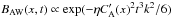 , where symbols have their usual meaning and
 denotes an Alfven speed derivative in the density inhomogeneity direction that runs across the background magnetic field (Heyvaerts & Priest 1983). The phase-mixing of AWs that have a Gaussian profile (as opposed to harmonic) along the background magnetic field has slower, power-law damping, BAW ∝ t− 3 / 2, as established by Hood et al. (2002). A mathematically more elegant derivation of the latter scaling law has been provided by Tsiklauri et al. (2003). The exponentially diverging magnetic field lines provide even faster damping BAW = exp(−A1exp(A2t)) (Similon & Sudan 1989; De Moortel et al. 2000; Smith et al. 2007). Malara et al. (2000) considered small-amplitude AW packets in Wentzel-Kramers-Brillouin (WKB) approximation in the Arnold-Beltrami-Childress (ABC) magnetic field. The latter can (for certain values of physical parameters) have exponentially diverging magnetic fields, thus also providing a superfast (exponent of exponent) AW dissipation. Tsiklauri (2014) studied the dissipation of AW in ABC fields using 3D magnetohydrodynamic (MHD) simulations (without a WKB restriction) and found that perturbation energy grows in time. This was attributed to a new instability, whose growth rate appears to be dependent on the value of the resistivity and the spatial scale (wavelength) of the AW. Nakariakov et al. (1998) studied the nonlinear coupling of MHD waves in a cold, compressible plasma with a smoothly inhomogeneous low-speed steady flow that was directed along the magnetic field in the phase-mixing context. Their main focus, however, was on the wave-mode coupling rather than a possibility that the flow reduces the effect of phase-mixing, which we consider here.
The OMFS in the solar corona – and possibly in coronae of other similar stars – come in different forms. We refer to the “openness” of the magnetic field in a sense that the structure must be able to sustain a background flow. These can be chromospheric upflows induced by magnetic reconnection in long coronal loops (long enough for the magnetic field to be treated as uniform, to simplify our model) or coronal polar plumes. Generally, a distinction is drawn between coronal holes (Golub & Pasachoff 2009), plumes (Deforest et al. 1997; Del Zanna et al. 1997; Raouafi et al. 2007) and more recently dark jets (Young 2015).
The solar coronal holes (CH) are regions of low-density and low-temperature (compared to the background) plasma, which are believed to be a source for fast (≈800 km s-1) solar wind, (see Chap. 4.9 in Aschwanden 2005. CH temperature is typically 0.8–0.9 MK compared to surrounding quiet corona that has a temperature of 0.9–1.2 MK. The boundaries of CH can be clearly seen in soft X-ray images, because of the absence of hot 1.2–1.5 MK plasma in them, when compared to the background.
The solar coronal polar plumes (CPPs) are radial, thin elongated structures that are visible in white light eclipse photographs as enhancements of density (3–6 times denser than the background), usually located inside coronal holes (Del Zanna et al. 1997). Because they are denser means that the plumes appear brighter than the surrounding media. In extreme ultraviolet (EUV) spectroheliograms they appear as shorter spikes near the polar limb. Some models and observations suggest that the plume plasma remains much slower and cooler than inter-plume plasma up to 2.0 R⊙. Values above these plasma parameters start to approach the inter-plume values, matching them at about 3.0 R⊙. The flow speed and temperature increase of the plasma inside plumes is sometimes observed (Raouafi et al. 2007). The latter work explains the flow speed and temperature increase by a possibility of interaction of the CPP’s core with the faster and hotter inter-plume material. Generally, it is debatable whether CPP is the source of fast solar wind (see related discussion and references in Deforest et al. 1997). Ultimately, this is related to the question of whether CPPs have small dipolar magnetic field patches at their base or are unipolar. Extensive work by Deforest et al. (1997) suggests that CPP have unipolar magnetic fields. Their Fig. 9, however, shows that, despite the magnetic field being unipolar, it is still patchy, or, and this is crucial for our model, the Alfvén speed varies across the magnetic field, giving rise to the phase-mixing of AWs. Also, on the theoretical side, Ofman & Davila (1997) have shown that torsional AWs generate solitary waves non-linearly and these may play a crucial role in fast solar wind acceleration, which is a separate issue.
The solar coronal dark jets (DJs) are relatively new features (Young 2015). The coronal jets have been known for some time to be a feature of solar coronal hole observations obtained in X-ray or EUV wavelengths. Young (2015) shows examples of DJs that are essentially invisible in EUV image sequences but have a clear signature in Dopplergrams derived from an EUV emission line. Interestingly, Cirtain et al. (2007) provide evidence for Alfvén waves in solar X-ray jets.
Chapter 8.2.3 in Aschwanden (2005) provides an overview of observations of Alfvén waves in OMFS. Because AW do not perturb density, they can be detected using spectral observations. The non-thermal broadening of EUV coronal lines typically shows bulk plasma speeds of 30 km s-1 (Doyle et al. 1998). For a typical AW phase speed of 1000 km s-1, this means that AWs in OMFS have amplitudes of 3% of the background. Therefore AWs in OMFS are weakly non-linear. Different types of waves are present not only in the corona. Jess et al. (2012) use high spatial, spectral, and temporal resolution images, obtained using both ground- and space-based instrumentation, to investigate the coupling between wave phenomena observed at different heights in the solar atmosphere.
The motivation for this study is to include the effect of plasma flow in AW damping via phase-mixing and explore its observational implications. Section 2 provides the model and analytical calculations. Section 3 describes the two-dimensional (2D) MHD simulations that corroborate the analytical results. Section 4 lists the main conclusions and outlines suggestions for future observational validation of the theory that is formulated in this work.
2. The model and analytical calculations
We describe AW dynamics using MHD equations for cold (the background pressure is equal to zero, p0 = 0), incompressible (density perturbation is equal to zero, ρ′ = 0) plasma with non-zero resistivity and zero viscosity (η ≠ 0, ν = 0): 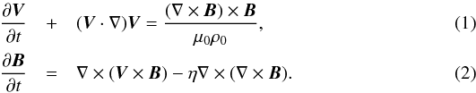 The background plasma quantities are denoted with subscript 0, while perturbation (AW) are denoted with primes as follows: V0 = (0,V0,0), B0 = (0,B0,0), ρ0 = ρ0(x), and
  ,
,  . The z-coordinate is assumed to be an ignorable direction, i.e. ∂/∂z = 0.
Linearly polarised AW is described by the z-component of Eqs. (1) and (2): 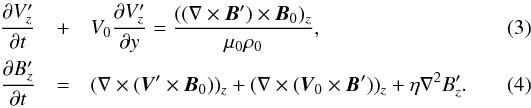 In Eq. (4), the vector identity ∇ × (∇ × B) = ∇(∇·B)−∇2B has been used with the divergence of the magnetic field being zero (∇·B = 0). Therefore, the system of equations that describes AW dynamics (and dissipation) is as follows
 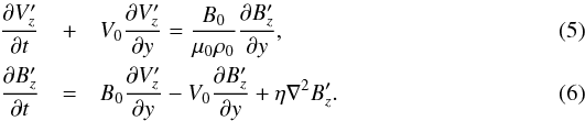 Next, we transform the equations into the frame co-moving with AW plus background flow speeds with the following coordinates
  :
:  , ξ = y−CA(x)t − V0(x)t and τ = εt (with ε ≪ 1). The derivatives in the new coordinate system are as follows:
 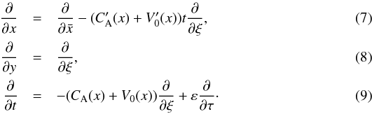 Applying the transform to the linearized first order system of Eqs. (5) and (6), and algebraically cancelling the terms that contain V0 yields
 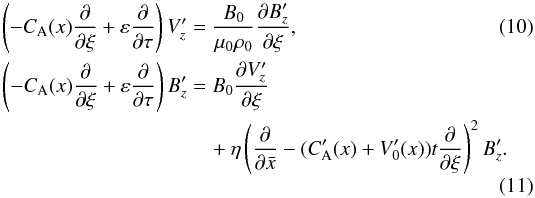 In Eq. (11) in the ∇2 = ∂2/∂x2 + ∂2/∂y2 we only kept ∂2/∂x2 because of the phase-mixing ∂2/∂x2 ≫ ∂2/∂y2. The next step is to apply operator −CA(x)∂/∂ξ + ε∂/∂τ to Eq. (11):
 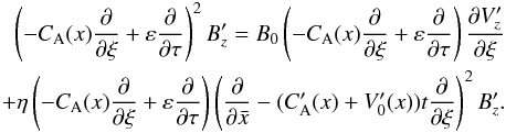 (12)We then apply operator ∂/∂ξ to Eq. (10)
 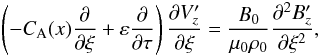 (13)and substitute the latter into Eq. (12).
 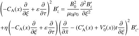 (14)
(14)
Equation (14) is an equation for  and can be solved analytically using simplifying assumptions in the asymptotic limit of large time t/τA ≫ 1. Here τA is the Alfvén time τA = L/CA(x), with L and CA(x) = B0/ (μ0ρ0(x))0.5 being a typical lengthscale of the system and Alfvén speed, respectively. Ignoring ε2 ≪ 1 order terms, whilst retaining only t2 ≫ 1 order terms in the term proportional to η, yields
 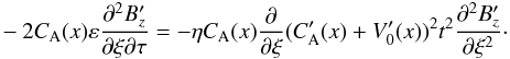 (15)In the above equation, the term
  algebraically cancels out.
As in Tsiklauri et al. (2003), we now introduce an auxiliary quantity that has a physical meaning of slow diffusion time for an AW: 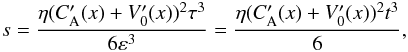 (16)and the derivative
 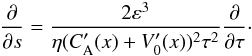 (17)Using the new notation and after integration by ξ, Eq. (15) reduces to the diffusion equation
  (18)Following similar approach as in Tsiklauri et al. (2003), Eq. (18) can be integrated as
 ![\begin{eqnarray} B_z={\frac {1} {2 \sqrt{\pi s}}} \int_{-\infty}^{+\infty} \exp \left[{-{\frac{(\xi-\xi')^2}{4 s}}}\right] \, B_z(\xi',t=0) \, {\rm d} \, \xi'. \label{19} \end{eqnarray}](/articles/aa/full_html/2016/02/aa27105-15/aa27105-15-eq67.png) (19)Let us substitute a harmonic wave initial condition Bz(ξ′,t = 0) = exp(ikξ′) into Eq. (19). The integration provides a solution
(19)Let us substitute a harmonic wave initial condition Bz(ξ′,t = 0) = exp(ikξ′) into Eq. (19). The integration provides a solution  (20)Equation (20) generalises the well known Heyvaerts & Priest’s solution for the case of shear flow, which is modified by the following substitution
  .
.
For a Gaussian pulse of the following mathematical form, Bz(ξ′,t = 0) = α0e− ξ′2/ 2σ2, its substitution into Eq. (19) gives a solution ![\begin{eqnarray} \nonumber &&B_z={\frac{\alpha_0}{ \sqrt{1+ \eta (C_{\rm A}^\prime(x)+V_0^\prime(x))^2 t^3/ 3 \sigma^2}}} \\ &&\quad\quad\times \exp{\left[{-{\frac{[y-(C_{\rm A}(x)+V_0(x)) t]^2}{2 (\sigma^2+ \eta (C_{\rm A}^\prime(x)+V_0^\prime(x))^2 t^3/ 3)}}}\right]}, \label{21} \end{eqnarray}](/articles/aa/full_html/2016/02/aa27105-15/aa27105-15-eq72.png) (21)which generalises the solutions that have been obtained before (Hood et al. 2002; Tsiklauri et al. 2003). Here, α0 = 1/
(21)which generalises the solutions that have been obtained before (Hood et al. 2002; Tsiklauri et al. 2003). Here, α0 = 1/ . In the asymptotic limit of large times, t, Eq. (21) implies that the amplitude of AW Gaussian pulse damps as
 ![\begin{eqnarray} B_z= \frac{1}{5} \left[2 \pi \eta (C_{\rm A}^\prime(x)+ V_0^\prime(x))^2/3\right]^{-1/2}\,t^{-3/2}. \label{22} \end{eqnarray}](/articles/aa/full_html/2016/02/aa27105-15/aa27105-15-eq76.png) (22)
(22)
3. Two-dimensional MHD simulations
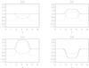 |
Fig. 1 Alfvén (CA(x), dashed curve) and background plasma flow (V0(x), dotted curve) speeds as a function of x-coordinate (across the magnetic field). Solid curve shows the sum of the two CA(x) + V0(x). The different panels show cases of a)D = 1, flat total speed profile across x-coordinate (no phase-mixing); b)D = 2, forward flow exceeding AW speed; c)D = 3 stronger forward flow, further exceeding the AW speed; and d)D = −1 backward flow. |
The 2D MHD numerical simulations of this work employ Lare2d Arber et al. (2001) – a Lagrangian remap code that solves non-linear MHD equations1. Lare2d is second-order accurate in space and time. Lare2d uses shock viscosity and gradient limiters to capture shock. However, the amplitudes considered in this work are weakly non-linear. In all our numerical simulations we use a 2D box with 3000 × 24 000 uniform grids in x and y direction, which have alength of 2π and 16π in each spatial direction, respectively. The distance, magnetic field, and density are normalised to their background values L,B0,ρ0. The velocity and time are normalised to the corresponding Alfvén values CA = B0/ and τA = L/CA at x = 0. Boundary conditions are periodic in both spatial directions. In all numerical runs, a normalised, uniform magnetic field, of strength unity, is in y-direction. The density has a profile in x-direction ρ(x) = 1 + 9exp(−(x − π)4). Therefore, a normalised Alfvén speed profile is
 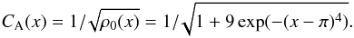 (23)Plasma beta and gravity are set to zero in all numerical runs. For numerical reasons, plasma beta is actually set to 10-8, but effectively it is zero. In all our simulations with AWs at t = 0 we impose a Gaussian pulse which has two components, Bz = 0.01exp(−(y−0.5)2/ (2 × 0.052)),
  , making it a linearly polarised AW packet with an amplitude of 0.01. The pulse starts at y = 0.5 and has a width of σ = 0.05. Only in Fig. 7 the pulse starts at y = 8, so that the backflowing middle part stays within the simulation domain. Plasma viscosity is set to zero, while first and second shock viscosity coefficients are set at 0.01 and 0.05 (see Arber et al. 2001 for further details). The plasma resistivity is always set to
  . The resistivity is quoted in units of μ0LCA. Therefore, 1/
 is the Lundquist number. Plasma flow runs along y-direction and its mathematical form is given by
  (24)with constant D = 0,1,2,3 or D = −1 controlling the cases of (i) no flow (usual phase-mixing, Hood et al. 2002; Tsiklauri et al. 2003); (ii) flat profile across x-coordinate (no phase mixing); (iii) forward flow, exceeding AW speed; (iv) stronger forward flow, further exceeding AW speed; and (v) backward flow, respectively. Each numerical run takes about five hours on 256 CPU computing cores on a COSMA-5 supercomputer2. The different examples are illustrated in Fig. 1. It follows from Fig. 1a that for the chosen set of parameters, Alfvén wave (CA(x), dashed curve) in the over-dense region 1.5 <x< 4.5 lags with min(CA(x)) = 0.3162. For D = 1, the background plasma flow (V0(x), dotted curve) speed has a maximum max(V0(x)) = 1–0.3162 = 0.6838 in the same region, such that the sum of the two CA(x) + V0(x) = 1 (solid curve) for all x. The same follows from the analytical expressions Eqs. (23) and (24), i.e. for D = 1 the CA(x) terms cancel out. Thus, D = 1 case corresponds to a flat profile across x-coordinate (no phase-mixing). In other words the forward flow completely counteracts the wave-front stretching because of the variation of Alfvén speed with the transverse coordinate. Figure 1b is for D = 2, forward flow, whose speed exceeds AW speed reduction, such that max(V0(x)) = 1.3675 and max(CA(x) + V0(x)) = 1.6838. The velocity sum difference between over-dense and peripheral regions in Fig. 1b is 1.6838–1 = 0.6838, the same as the Alfvén speed decrease 1–0.3162 = 0.6838. In other words, in Fig. 1b, the solid and dashed lines are perfectly symmetrical with respect to y = 1. Figure 1c is for D = 3, even stronger forward flow, such that max(V0(x)) = 2.0513 and max(CA(x) + V0(x)) = 2.3675. Figure 1d is for D = −1 backward flow, such that min(V0(x)) = −0.6838 and min(CA(x) + V0(x)) = −0.3675. The velocity sum difference between over-dense and peripheral regions in Fig. 1c is 2.3675–1 = 1.3675, the same as that in Fig. 1d 1−(−0.3675) = 1.3675. In other words, in Figs. 1c and 1d, the solid curves have the same gradient strength, which is also clear visually.
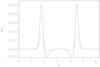 |
Fig. 2 Difference between background flow speed at time t as a function of x-coordinate, V0(x,y = ymax/ 2,t), and its initial value at t = 0, V0(x,y = ymax/ 2,0), i.e. ΔVy ≡ V0(x,y = ymax/ 2,t) − V0(x,y = ymax/ 2,0) for different time instances. Dashed curve corresponds to t = 5, dotted to t = 10 and solid to t = 20. This numerical run is considered for the fastest background flow, with D = 3 (as in panel c from Fig. 1). It is clear that by t = 20 the flow speed difference is very small ≈0.005, i.e. the flow stays intact and does not disintegrate. |
In Fig. 2 we plot the difference between background flow speed at time t as a function of x-coordinate, V0(x,y = ymax/ 2,t) and its initial value at t = 0, V0(x,y = ymax/ 2,0), i.e. ΔVy ≡ V0(x,y = ymax/ 2,t) − V0(x,y = ymax/ 2,0) for different times. The dashed curve is for t = 5, while the dotted curve is for t = 10 and solid for t = 20. In this numerical run the background flow is the fastest of all the performed numerical runs with D = 3 (as in panel (c) from Fig. 1). We gather from Fig. 2 that, by the end simulation time of t = 20, the flow speed difference is quite small, ≈ 0.005. It is even smaller for earlier times and/or smaller values of D. Therefore in Fig. 2, we demonstrate that the background flow in the absence of the AW pulse does not break up.
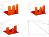 |
Fig. 3 Shaded surface plots of Bz(x,y) at different times for the case without the flow D = 0. Panel a) is for t = 5; b) for t = 10; and c) for t = 20. Panel d) is time evolution of AW amplitude, normalised to its initial value, for the same case. The solid line corresponds to the asymptotic solution for large times, Eq. (22), at the strongest density gradient point x = (907 / 3000) × 2π = 1.8996. A more general analytical form Eq. (21) is plotted with dashed curve for the same x value (we actually plot Bz(1.8996,y) /α0). Crosses and open diamonds are MHD numerical simulation results in the strongest density gradient point x = (907 / 3000) × 2π = 1.8996 and away from the gradient x = (1 / 3000) × 2π = 0.0021 (the first grid cell in x-direction), respectively, by tracing the maximum value of the Gaussian AW pulse. Dash-triple-dotted line corresponds to the asymptotic solution for large times, Eq. (31), which is independent of x. A more general analytical form Eq. (30) is plotted with dash-dotted curve. It is also independent of x because at the peak of the pulse the value of exponent is unity. |
Figure 3 shows the numerical run results for the case of no background flow with D = 0. This corresponds to a similar set-up studied in Hood et al. (2002), Tsiklauri et al. (2003) or more recently in Tsiklauri (2014), as the numerical code benchmarking exercise. Figure 3 shows shaded surface plots of the AW, i.e. Bz(x,y) at different times. Panel a is for t = 5; b for t = 10; and c for t = 20. Panel d shows the time evolution of AW amplitude, normalised to its initial value. The solid line corresponds to the asymptotic solution for large times, Eq. (22). A more general analytical form Eq. (21) is plotted with a dashed curve. Crosses and open diamonds represent numerical simulation results in the strongest density gradient point x = (907 / 3000) × (2π) = 1.8996 and away from the gradient x = (1 / 3000) × (2π) = 0.0021 (the first grid cell in x-direction), respectively. The Dash-triple-dotted line corresponds to the asymptotic solution for large times, Eq. (31), which is independent of x. A more general analytical form of Eq. (30) is plotted with a dash-dotted curve. It is also independent of x because, at the peak of the pulse, the value of the exponent is unity. At t = 0 (snapshot not shown here) AW is initially flat as in, e.g. Fig. 4a, but without the hump in the middle and instead it is located at y = 0.5, according to the initial conditions given above. The Alfvén wavefront quickly damps (the shaded surface disappears from 3a to 3c in the density inhomogeneity regions x ≈ 1.5–2.5 and x ≈ 3.5–4.5, where the wave fronts distort strongly. The derivative of the Alfven speed, , in x-direction, which enters Eqs. (21) and (22), with V0 = 0 and  as D = 0, is responsible for the fast damping of the AW. Away from the density gradient regions, a much slower dissipation takes place. The latter is hardly noticeable on the timescales concerned (0 <t< 20). Away from the density gradient regions, the analytical solutions Eqs. (30) and (31) seem to match the corresponding numerical solution (open diamonds) well.
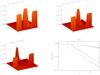 |
Fig. 6 Same as in Fig. 3 but for the case of D = 3. The dotted line corresponds to the asymptotic solution for large times, Eq. (22), at the strongest density gradient point x = (907 / 3000) × (2π) = 1.8996, while solid line and dashed curve are kept the same as in Fig. 3 for comparison. |
In Fig. 4 we present numerical run results in a similar manner to Fig. 3, except that D = 1. Note that in panel 4d we have adjusted the plot y-range to 0.4–1.4 to see the amplitude behaviour more clearly. At all times, we see that the AW front remains flat across x-coordinate, and the phase-mixing effect is absent. Thus, for over-dense plasma structures, which have smaller CA compared to the surrounding plasma, the plasma flow that is confined to this structure and running in the same direction as the AW, reduces the effect of phase-mixing because, on the edges of the structure,  and
and  have the opposite signs. In fact, we deduce from Eqs. (23) and (24) that for D = 1, CA(x) + V0(x) = 1 =const and therefore
  . Thus, the rather slow wave damping is not due to phase-mixing but to the usual Spitzer resistivity (note the crosses nearly coincide with open diamonds in Fig. 4d). This small mismatch, of the order of 0.0008, could be due to the two following reasons: (i) AW has two components (Vz, Bz) and, as stated above, the initial condition for Vz is . Thus, despite the fact that the wave front is flat, because of the presence of the flow, the density is still a function of transverse coordinate x; (ii) for the latter reason, the non-linearity will damp the wave front in a slightly different way. Although, our analytical problem is linear, we validate it with a fully non-linear MHD code Lare2d. In Fig. 2, the maximal flow difference ΔVy is approximately 0.005. Thus, the small mismatch of ≈0.0008 could be attributed mostly to the non-linearity of the numerical code. We stress that the plasma resistivity is always set to everywhere. Consequently, the small difference is not due to the weak (logaritm of plasma parameter) density dependence of the Spitzer resistivity being affected by the background density profile. Thus, the wave damps only by Spitzer (uniform) resistivity not by phase-mixing. This is the result of the co-directional flow, which reduces the wave front stretching in the transverse direction to zero, while the front remains flat across x at all times.
Figure 5 shows numerical run results similar to those found in Fig. 3, except for D = 2. The choice of value of D is such that wave front in Figs. 5a–c now bends forward instead of backward compared to Fig. 3a–c. We notice that Fig. 5d seems identical to 3d. This is because the AW-amplitude damping, using the phase-mixing formula Eqs. (22), contains the square of the sum of the Alfvén and flow speed derivatives. In the case of Fig. 3, the wave front derivative is negative in the density inhomogeneity regions x ≈ 1.5–2.5, while in the case of Fig. 5, it is positive. However, since the derivative is squared, the net effect is the same – the case without a flow and with forward flow with D = 2, the AW damping is the same.
In Fig. 6 we present numerical run results similar to those found in Fig. 3, except for D = 3. This is the strongest flow case we consider and it demonstrates that fast flow can induce wave front stretching to the extent that it exceeds the usual effect of phase-mixing without a flow. The latter can be clearly seen by looking at the crosses and the dotted line in Fig. 6d, which appear lower than the solid line, thus indicating a stronger damping, as prescribed by Eqs. (21) and (22).
Figure 7 depicts the numerical run results as in Fig. 6, except for D = −1. This corresponds to the back-flow case, i.e. the AW propagates in the opposite direction to the background flow. Compared to the case without the flow, Figs. 3a–c, in Fig. 7a–c we see the AW stretching is stronger and therefore the wave damping via the phase-mixing is faster. However, the damping is the same as in the case where D = 3. Therefore Fig. 7d appears identical to 6d.
To summarise, based on Eqs. (23) and (24), CA(x) + V0(x) = D + (1 − D)CA(x), and therefore, 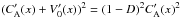 . The latter prescribes the AW damping via phase-mixing in Eqs. (21) and (22). Thus,
-
 for D = 0 (Fig. 3);
 -
0 for D = 1 (Fig. 4);
-
for D = 2 (Fig. 5);
-
 for D = 3 (Fig. 6);
 -
for D = −1 (Fig. 7).
Thus, the AW damping via phase-mixing is the same in the cases of D = 0 and D = 2, and similarly for cases D = 3 and D = −1. For D = 1, the phase-mixing effect is zero. Note that phase-mixing always acts in addition to the usual (homogeneous plasma case) resistive damping, which diffuses the AW pulse in the other spatial direction (in y). This can be seen by the slight broadening of the pulse in y direction in Figs. 3–7.
To quantify the AW Gaussian pulse damping in the homogeneous plasma case, we now consider a one-dimensional (1D) analogue of our 2D model by suppressing the variation in x-direction. Therefore we consider a 1D AW pulse moving along y in homogeneous plasma. In this case Eq. (14) is replaced by 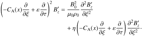 (25)Here,
 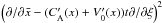 operator has been replaced by ∂2/∂y2 = ∂2/∂ξ2 because in the 2D phase-mixing case in Eq. (14), we set ∂2/∂x2 ≫ ∂2/∂y2, while in 1D case ∂/∂x = 0. This means that, out of the ∇2 operator, we retain ∂2/∂y2. Following a similar procedure, as described above, the equivalent form of Eq. (15) is now
 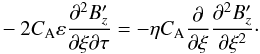 (26)We now introduce an auxiliary quantity,
  (27)Using the new notation and, after integration by ξ, Eq. (26) reduces to the diffusion equation
  (28)As above, Eq. (28) can be integrated using Eq. (19). For a Gaussian pulse of the following mathematical form, Bz(ξ′,t = 0) = α0e− ξ′2/ 2σ2, its substitution into Eq. (19) yields
 ![\begin{eqnarray} B_z^\prime=\frac{\alpha_0}{\sqrt{1+ 2s_1/ \sigma^2}} \exp{\left[{-{\frac{\xi^2}{2 (\sigma^2+ 2s_1)}}}\right]}\cdot \label{29} \end{eqnarray}](/articles/aa/full_html/2016/02/aa27105-15/aa27105-15-eq170.png) (29)Substituting the definition of s1 provides the desired solutions
(29)Substituting the definition of s1 provides the desired solutions ![\begin{eqnarray} B_z=\frac{\alpha_0}{\sqrt{1+\eta t / \sigma^2}} \exp{\left[{-{\frac{[y-(C_{\rm A}(x)+V_0(x)) t]^2}{2 (\sigma^2+ \eta t)}}}\right]}, \label{30} \end{eqnarray}](/articles/aa/full_html/2016/02/aa27105-15/aa27105-15-eq172.png) (30)and its asymptotic limit of large times:
(30)and its asymptotic limit of large times: ![\begin{eqnarray} B_z= \frac{1}{5} \left[2 \pi \eta \right]^{-1/2}\,t^{-1/2}. \label{31} \end{eqnarray}](/articles/aa/full_html/2016/02/aa27105-15/aa27105-15-eq173.png) (31)In the case of homogeneous plasma resistive damping of the Gaussian AW pulse, the amplitude damps as t− 1 / 2 compared to t− 3 / 2 for the 2D phase-mixing. In the uniform density regions, the analytical solutions Eqs. (30) and (31) seem to match the corresponding numerical solution (open diamonds) in all Figs. 3–7 well.
(31)In the case of homogeneous plasma resistive damping of the Gaussian AW pulse, the amplitude damps as t− 1 / 2 compared to t− 3 / 2 for the 2D phase-mixing. In the uniform density regions, the analytical solutions Eqs. (30) and (31) seem to match the corresponding numerical solution (open diamonds) in all Figs. 3–7 well.
4. Conclusions
This paper uses analytical calculations, corroborated by MHD simulations, to demonstrate that, when a flow is present, mathematical expressions for the Alfvén wave damping via phase-mixing are modified by the following substitution . In uniform magnetic field and over-dense plasma structures, in which CA is smaller compared to the surrounding plasma, the flow, which is confined to this structure, and in the same direction as the AW, reduces the effect of phase-mixing. This is because, on the edges of the structure, and have opposite signs. As a result of this, the AW damping, via phase-mixing, is slower when compared to the case without the flow. For example, in the over-dense plasma structures with density inside ten times higher than outside, the co-directional with the wave flow with ≈0.7CA in the middle of the over-density (see Figs. 1a and 4) can reduce the phase-mixing effect to zero. This is the consequence of the co-directional flow reducing the wave front stretching in the transverse direction to zero. Conversely, the counter-directional flow increases the wave front stretching in the transverse direction, therefore making the phase-mixing effect more effective (see Figs. 1d and 7) compared to the case without the flow. The flows with ≈1.4CA and ≈2CA in the middle of the over-density, make the wave front go faster in the over-dense region compared to the surrounding plasma (see Figs. 1b, 1c, 5 and 6). In the case without the flow (Fig. 3), the wave front is slower in the over-dense region compared to the surrounding plasma. The dissipation of the AW via phase-mixing is: (i) the same for flows with ≈1.4CA as for those without the flow (although in both cases the wave front is bent forward and backward, respectively); and (ii) larger for case of ≈2CA (which is probably unrealistic observationally, but is presented for completeness), as quantified by Eq. (22). We stress that the result is generic and is applicable to different laboratory or astrophysical plasma systems where flows, density inhomogeneity across the background magnetic field, and AW resistive dissipation are all present. Nonetheless, we apply our findings to address the question why over-dense solar coronal OMFS are cooler than the background plasma. Since observations show that the over-dense OMFS are cooler than the surrounding plasma, and that they are in regions where Doppler line-broadening is consistent with bulk plasma motions, e.g. the AW, we show that, if over-dense solar coronal OMFS are heated by AW damping via phase-mixing, the co-directional with the wave plasma flow in them reduces the phase-mixing-induced heating, thus providing an explanation for why they are cooler than the surrounding plasma.
As mentioned in the introduction, and reiterated here, there is currently a disagreement as to whether CPPs are the source of fast solar wind (see related discussion and references in Deforest et al. 1997). Some observations claim that the source of the fast solar wind is the inter-plume region. Giordano et al. (2000) present a spectroscopic study of the ultraviolet coronal emission in a polar hole. They identify the inter-plume lanes and background coronal hole regions as the channels in which the fast solar wind is preferentially accelerated. i.e. outside the plume the speed is higher than in the plume. We stress, however, that these observations only present three measurements of the flow speed: two on either side of the plume, where flow speed is found faster and one inside where flow speed is slower. This does not preclude a possibility that on the edges of the plume the flow speed falls to zero and thus  inside the plume. Since, in the over-dense structures with a uniform magnetic field
  , the effect of the flow counteracting the phase-mixing is still a viable possibility.
Harra et al. (2015) explored the changes in coronal non-thermal velocity (i.e. bulk flows or AWs) measurements at the poles from solar minimum to solar maximum, using Hinode EUV Imaging Spectrometer (EIS) data. They find that, although the intensity in the corona at the poles does tend to increase with the cycle, there are no significant changes in the Vnon−thermal values. The locations of enhanced Vnon−thermal values that they measure do not always have a counterpart in intensity, and they are sometimes located in weak emission regions. The next logical step in corroborating our theory would be to check whether there is a correlation between temperature and non-thermal velocity in over- or under-dense OMFS. Care should be taken however in interpreting the observational results. We considered over-dense structures (e.g. coronal plumes) and found that, co-directional with the wave flows reduce phase-mixing and hence reduce heating/wave-dissipation, such that they appear cooler than their surroundings. Obviously, in under-dense structures, where AW phase speed inside the structure is higher, hence co-directional with the wave flows increase the phase mixing and thus increase wave-dissipation/temperature. This would result in a positive correlation between proton temperature and solar wind speed Tu & Marsch (1994; Horbury & Matteini, priv. comm.), i.e. faster streams are also hotter. Typically during periods of fast solar wind (V> 700 km s-1), with fast streams (V = 150–200 km s-1), both the total magnetic field and the density are constant. Thus Alfvén speed is constant across the streams. Matteini et al. (2015) show that in terms of the turbulence, the system appears to be in a local equilibrium, where there are no jumps in particle/field energies. This behaviour suggests that the turbulence has evolved to a stage where the system is in equilibrium, making fast streams and background homogeneous. However, assuming that at the origin there were independent steams of plasma, with different physical properties, it is plausible that Alfvén speed is different in different streams. It is likely that the condition | B | = const. (Matteini et al. 2015) is the result of the relaxation of the turbulence and not the initial configuration, where jets could have had different B0, which has subsequently been smoothed out. The next logical step would be to do a careful pressure-balance calculation, taking into account the temperature changes.
Thus, based on our model, the ultimate factor for interpreting the observations is dependent on whether Alfvén speed (which is a combination of both density and the magnetic field) is smaller or larger than in the surrounding plasma. In summary, when plotting a graph of coronal non-thermal velocity, Vnon−thermal, i.e. the background flow speed, versus temperature inside the structure, T, based on, e.g. EIS (Hinode)/ AIA (Solar Dynamics Observatory) observations in the solar corona or Helios observations in fast solar wind streams, the model predicts:
-
a positive correlation of Vnon−thermal with T in the case of structures in which Alfvén speed is larger compared to the surrounding plasma;
-
anti-correlation of Vnon−thermal with T in the case of structures in which Alfvén speed is smaller compared to the surrounding plasma (hence the title of this paper).
These conclusions are based on natural assumptions that (i) AW phase-mixing has a major role to play in heating these structures; and (ii) that the flow is forward (co-directional) with the AW (i.e. solar wind). There is also a caveat that in the above correlation, Vnon−thermal means background flow rather than AW or turbulent motions, and that the disentangling of the two maybe difficult. This is maybe easier on the solar disk rather than on the limb, because measuring Doppler shifts should enable us to differentiate between regular (up- or down-) flows from bulk turbulent motions, which only manifest themselves via the line broadening.
The code is available for download from http://ccpforge.cse.rl.ac.uk/gf/project/lare2d/
Acknowledgments
Computational facilities: Astronomy Unit, Queen Mary University of London and UK’s STFC Dirac-2 HPC via UKMHD consortium. The author was financially supported by STFC consolidated Grant No. ST/J001546/1 and Leverhulme Trust Research Project Grant No. RPG-311. The author would also like to thank Dr. T. R. Arter for providing crucially important IT support.
References
- Arber, T. D., Longbottom, A. W., Gerrard, C. L., & Milne, A. M. 2001, J. Comp. Phys., 171, 151 [Google Scholar]
- Aschwanden, M. J. 2005, Physics of the Solar Corona. An Introduction with Problems and Solutions (2nd edn.), Chap. 9.4 (Berlin Heidelberg: Springer-Verlag) [Google Scholar]
- Cirtain, J. W., Golub, L., Lundquist, L., et al. 2007, Science, 318, 1580 [NASA ADS] [CrossRef] [PubMed] [Google Scholar]
- De Moortel, I., Hood, A. W., & Arber, T. D. 2000, A&A, 354, 334 [NASA ADS] [Google Scholar]
- Deforest, C. E., Hoeksema, J. T., Gurman, J. B., et al. 1997, Sol. Phys., 175, 393 [NASA ADS] [CrossRef] [Google Scholar]
- Del Zanna, L., Hood, A. W., & Longbottom, A. W. 1997, A&A, 318, 963 [NASA ADS] [Google Scholar]
- Doyle, J. G., Banerjee, D., & Perez, M. E. 1998, Sol. Phys., 181, 91 [NASA ADS] [CrossRef] [Google Scholar]
- Giordano, S., Antonucci, E., Noci, G., Romoli, M., & Kohl, J. L. 2000, ApJ, 531, L79 [NASA ADS] [CrossRef] [Google Scholar]
- Golub, L., & Pasachoff, J. M. 2009, The Solar Corona (Cambridge: Cambridge University Press) [Google Scholar]
- Harra, L., Baker, D., Edwards, S. J., et al. 2015, Sol. Phys., 290, 3203 [NASA ADS] [CrossRef] [Google Scholar]
- Heyvaerts, J., & Priest, E. R. 1983, A&A, 117, 220 [NASA ADS] [Google Scholar]
- Hood, A. W., Brooks, S. J., & Wright, A. N. 2002, Roy. Soc. London Proc. Ser. A, 458, 2307 [Google Scholar]
- Jess, D. B., De Moortel, I., Mathioudakis, M., et al. 2012, ApJ, 757, 160 [NASA ADS] [CrossRef] [Google Scholar]
- Malara, F., Petkaki, P., & Veltri, P. 2000, ApJ, 533, 523 [NASA ADS] [CrossRef] [Google Scholar]
- Matteini, L., Horbury, T. S., Pantellini, F., Velli, M., & Schwartz, S. J. 2015, ApJ, 802, 11 [NASA ADS] [CrossRef] [Google Scholar]
- Nakariakov, V. M., Roberts, B., & Murawski, K. 1998, A&A, 332, 795 [NASA ADS] [Google Scholar]
- Ofman, L., & Davila, J. M. 1997, ApJ, 476, 357 [NASA ADS] [CrossRef] [Google Scholar]
- Raouafi, N.-E., Harvey, J. W., & Solanki, S. K. 2007, ApJ, 658, 643 [NASA ADS] [CrossRef] [Google Scholar]
- Similon, P. L., & Sudan, R. N. 1989, ApJ, 336, 442 [NASA ADS] [CrossRef] [Google Scholar]
- Smith, P. D., Tsiklauri, D., & Ruderman, M. S. 2007, A&A, 475, 1111 [NASA ADS] [CrossRef] [EDP Sciences] [Google Scholar]
- Tsiklauri, D. 2014, Phys. Plasmas, 21, 052902 [NASA ADS] [CrossRef] [Google Scholar]
- Tsiklauri, D., Nakariakov, V. M., & Rowlands, G. 2003, A&A, 400, 1051 [NASA ADS] [CrossRef] [EDP Sciences] [Google Scholar]
- Tu, C.-Y., & Marsch, E. 1994, J. Geophys. Res., 99, 21481 [NASA ADS] [CrossRef] [Google Scholar]
- Young, P. R. 2015, ApJ, 801, 124 [NASA ADS] [CrossRef] [Google Scholar]
All Figures
|
Fig. 1 Alfvén (CA(x), dashed curve) and background plasma flow (V0(x), dotted curve) speeds as a function of x-coordinate (across the magnetic field). Solid curve shows the sum of the two CA(x) + V0(x). The different panels show cases of a)D = 1, flat total speed profile across x-coordinate (no phase-mixing); b)D = 2, forward flow exceeding AW speed; c)D = 3 stronger forward flow, further exceeding the AW speed; and d)D = −1 backward flow. |
| In the text | |
|
Fig. 2 Difference between background flow speed at time t as a function of x-coordinate, V0(x,y = ymax/ 2,t), and its initial value at t = 0, V0(x,y = ymax/ 2,0), i.e. ΔVy ≡ V0(x,y = ymax/ 2,t) − V0(x,y = ymax/ 2,0) for different time instances. Dashed curve corresponds to t = 5, dotted to t = 10 and solid to t = 20. This numerical run is considered for the fastest background flow, with D = 3 (as in panel c from Fig. 1). It is clear that by t = 20 the flow speed difference is very small ≈0.005, i.e. the flow stays intact and does not disintegrate. |
| In the text | |
|
Fig. 3 Shaded surface plots of Bz(x,y) at different times for the case without the flow D = 0. Panel a) is for t = 5; b) for t = 10; and c) for t = 20. Panel d) is time evolution of AW amplitude, normalised to its initial value, for the same case. The solid line corresponds to the asymptotic solution for large times, Eq. (22), at the strongest density gradient point x = (907 / 3000) × 2π = 1.8996. A more general analytical form Eq. (21) is plotted with dashed curve for the same x value (we actually plot Bz(1.8996,y) /α0). Crosses and open diamonds are MHD numerical simulation results in the strongest density gradient point x = (907 / 3000) × 2π = 1.8996 and away from the gradient x = (1 / 3000) × 2π = 0.0021 (the first grid cell in x-direction), respectively, by tracing the maximum value of the Gaussian AW pulse. Dash-triple-dotted line corresponds to the asymptotic solution for large times, Eq. (31), which is independent of x. A more general analytical form Eq. (30) is plotted with dash-dotted curve. It is also independent of x because at the peak of the pulse the value of exponent is unity. |
| In the text | |
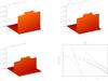 |
Fig. 4 Same as in Fig. 3 but for the case of D = 1. |
| In the text | |
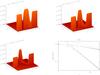 |
Fig. 5 Same as in Fig. 3 but for the case of D = 2. |
| In the text | |
|
Fig. 6 Same as in Fig. 3 but for the case of D = 3. The dotted line corresponds to the asymptotic solution for large times, Eq. (22), at the strongest density gradient point x = (907 / 3000) × (2π) = 1.8996, while solid line and dashed curve are kept the same as in Fig. 3 for comparison. |
| In the text | |
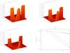 |
Fig. 7 Same as in Fig. 6 but for the case of D = −1. |
| In the text | |
Current usage metrics show cumulative count of Article Views (full-text article views including HTML views, PDF and ePub downloads, according to the available data) and Abstracts Views on Vision4Press platform.
Data correspond to usage on the plateform after 2015. The current usage metrics is available 48-96 hours after online publication and is updated daily on week days.
Initial download of the metrics may take a while.