© ESO, 2015

1. Introduction

Galactic globular clusters play an important role in helping us to understand the extent, formation, and evolution of our Galaxy. In particular, the kinematical information of the globular clusters is a step towards understanding the dynamics of the Galaxy. Proper motions (PMs) of the stars provide velocity information in two orthogonal directions (Sagar & Bhatt 1989) and enable us to determine membership status of the stars in the clusters.

According to Zinn (1985), Galactic globular clusters can be classified into two distinct systems. The first is the halo system, which contains metal-poor clusters having small net rotation and large velocity dispersion. The halo system globular clusters are approximately spherically distributed in the Galaxy. The other component is the disk system which is a flat system of metal-rich clusters with substantial rotation. The transition from one kinematic system to the other appears to occur abruptly at an abundance of approximately [Fe/H] = −0.8 dex. The basic results by Zinn (1985) were confirmed and extended by Armandroff (1989). These studies suggest that the most metal-rich globular clusters can be used to trace the halo-disk transition. Among the transition region clusters, NGC 6366 is a heavily reddened globular cluster located at approximately R_gc = 5 kpc, and z = 1 kpc towards the north Galactic pole (Webbink 1985; Alonso et al. 1997). In spite of the position of the cluster in the Galaxy and high reddening favoring disk-like rotation, its kinematical parameters derived by Da Costa & Seitzer (1989) do not agree with disk like rotation, and so they associated it with the halo system. It is interesting to see whether one can kinematically classify this cluster as a halo or a disk object. For this, it is preferable to use the cluster member stars to determine the space motion characteristics of the cluster. Therefore, determining membership probabilities of the stars is a crucial requirement to kinematically classify NGC 6366.

Precise wide-field astrometric surveys of globular clusters are important for many reasons. In the multislit and multifiber spectroscopic facilities, an accuracy of 0.2 arcsec or better is essential to position point-like sources in the slits/fibers. The mosaic-like CCD camera as wide field imager (WFI) mounted on the 2.2 m ESO telescope allows astrometric measurements with an accuracy far better than the nominal 0.2 arcsec (Anderson et al. 2006). A particularly useful application of astrometry, however, is to determine proper motions for a large number of stars.

NGC 6366 is a relatively unstudied globular cluster in the Milky Way. The cluster has been the subject of a few photometric and spectral studies (Pike 1976; Mould et al. 1979; Da Costa & Seitzer 1989; Alonso et al. 1997; Paust 2009; Campos et al. 2013). Thompson (2013) predicted that the cluster may harbor planetary systems. Chen & Chen (2010) studied the morphological distortion of NGC 6366 and found that the cluster is experiencing heavy tidal stripping. Variable stars in the cluster have been studied by Sawyer (1940), Harris (1993), Lloyd et al. (2008), and Arellano Ferro et al. (2008). Johnston et al. (1996) presented the results of X-ray observations of the cluster with the ROSAT X-ray telescope. Using Chandra X-ray observatory data, Bassa et al. (2008) detected 14 X-ray sources in the cluster region, 5 of which were within the half-mass radius (2.92 arcmin) of NGC 6366. On the basis of optical counterparts, these authors identified two or three X-ray sources belonging to the cluster. It was suggested that the brightest X-ray source in NGC 6366 is an old nova.

In light of the above discussion, it can be stated that there is clearly a dearth of proper motion (PM) studies for this kinematically interesting cluster. The catalogue of absolute proper motions of globular clusters by Dambis (2006) lists the absolute proper motion values (μ_αcosδ = −3.90 ± 0.57 mas yr^-1, μ_δ = −6.13 ± 0.52 mas yr^-1) for NGC 6366. Despite its proximity (~3.5 kpc), most of the studies for NGC 6366 have been hindered by high reddening and contamination by field stars. Therefore, a catalogue with membership information covering a wide field centered on the cluster is very much needed. The archival data taken with the WFI at the 2.2 m ESO telescope enable us to derive proper motions by using an epoch gap of only a few years, deeper by several magnitudes, and covering a larger region (Anderson et al. 2006; Yadav et al. 2008; 2013; Bellini et al. 2009; Sariya et al. 2012). We selected the WFI at the 2.2 m ESO telescope because it is one of the first wide-field cameras available, thus it has a long time baseline in its public archive.

The main goal of the present study is to provide PMs and membership probabilities (P_μ) for a large number of bright stars in the region of NGC 6366. As discussed by Cudworth (1986; 1997), the need to confirm the cluster membership of unusual stars is very common. In globulars, the stars in questions may be UV-bright stars, spectroscopically peculiar giants, variables, or blue stragglers. Spectroscopists interested in faint cluster members would often like to have membership information before observing to avoid integrating for hours on field stars, but the membership data are often not available. Questions of the existence and characteristics of cluster halos also generally require membership information, as do luminosity and mass function. For these reasons, a catalogue with B,V,I magnitudes, PMs, and membership probabilities covering ~13 × 17 arcmin² is being made available for follow-up studies of the cluster NGC 6366.

The fundamental parameters of the cluster, taken from Harris (1996, 2010 edition) and Goldsbury et al. (2010; 2011) are listed in Table 1. The details of archival data and astrometric reduction procedures are provided in Sect. 2. Proper motions with color-magnitude diagrams (CMDs) of the cluster are discussed in Sect. 3. Section 4 presents the cluster membership analysis. In Sect. 5, our catalogue is used to check the membership status of known variables and X-ray sources. The catalogue of the present study is described in Sect. 6, while the conclusions of the present study are given in Sect. 7.

2. Data used and reduction procedures

Proper motions of the stars in the cluster region were determined using V filter images from the ESO archive¹. The images used in this work were acquired using the 2.2 m ESO/MPI telescope at La Silla, Chile. This telescope is equipped with a Wide Field Imager (WFI) camera. This camera contains a mosaic of 4 × 2, i.e., eight CCD chips, with 2048 × 4096 pixels each, making it possible to image an observational area of 34 × 33 arcmin².

The detailed log of observations is listed in Table 2. The first epoch of observations consists of two images in the B,V, and I filters each with 240 s exposure time taken on April 06, 2000. The observational run of the second epoch is presented by four images with 120 s exposure time each in V filter observed on June 05, 2003. Thus, the epoch gap between the data is ~3.2 yr. Values of seeing of the images used in this study lie between 1.0−1.5 arcsec, while airmass values are ~1.1.

2.1. Astrometric and photometric reductions

In order to reduce the mosaic CCD images, the methods prescribed by Anderson et al. (2006, hereafter Paper I) have been adopted. This procedure includes standard initial steps of de-biasing and flat-fielding. Point spread function (PSF) modeling of the images is a crucial factor for providing precise positions of the stars. As shown in Paper I, the shape of the PSF changes across the CCD chip. An array of 15 PSFs per CCD chip (3 across and 5 high) can represent this variability. To account for this, an array of empirical point spread functions (PSFs) were constructed to provide positions and fluxes of the objects in an image. The concept here is to save these PSFs in a look-up table on a very fine grid. The PSF is represented by a 201 × 201 grid that is supersampled by a factor of four with respect to the image pixels. The center of the PSF is at (101,101) and it extends out to 25 pixels from the center of the stars. An automated code (Paper I) is used to iteratively calculate the precise positions and instrumental fluxes for the brightest down to faintest stars.

The WFI on the 2.2 m telescope is affected by high levels of geometric distortion in the focal plane that effectively changes the pixel scale across the field of view. In Paper I, the geometric distortion corrections were calculated using dithered observations of the Galactic bulge in Baade’s window. For each chip, the corrections are noted in a 9 × 17 element look-up table. A bi-linear interpolation between the four closest grid points from the look-up table to the target point provides the distortion correction for any location of the target point. However, the distortion corrections can be less accurate near the edges of the image. Also, the possibility of instability of the distortions for the WFI increases the uncertainty in distortion corrections.

We adopted the local transformation approach to account for the above-mentioned imperfections in the distortion solution. In the local transformation approach, we find the transformations from one frame to other frame locally, i.e., with respect to some stars in our own images. It is appropriate to select the cluster stars for this purpose as cluster stars tend to have less internal dispersion than the field stars. The selection of reference stars can be made either by their location in the CMD or iteratively by the motion itself, or both. Once the positions are known in two frames, six-parameter linear transformations are used to transform the coordinates from one frame to another. This method corresponds to the classical plate-pair method, but it is more generalized in the sense of being usable to all possible combinations of the first- and second-epoch frames. The average of all displacements for inter-epoch transformations gives the relative PM of a target star. Measurement errors in PMs are calculated from the residuals about the average for each epoch, since such residuals should be free of PM effects. The formulae to calculate PMs and their errors are explained in Paper I.

2.1.1. Astrometric calibration

One of the aims of our study is to present the coordinates of stars in the International Celestial Reference System (ICRS) in the area of NGC 6366. The X,Y raw positions of each star in each frame were corrected for geometric distortion using the look-up table provided in Paper I, and averaged by means of a six-parameter linear transformation into a common reference frame. Online digitized sky ESO catalogue in SKYCAT software is then used to transform the averaged X,Y positions to right ascension (RA) and declination (Dec) in J2000.0 equinox using IRAF² tasks CCMAP and CCTRAN. The transformations have rms values of about 60 and 30 mas in RA and Dec, respectively. The quality of distortion solution and the relative stability of the intra-chip positions enable us to apply a single plate model that contains linear and quadratic terms and a small but significant cubic term in each coordinate. This solution also absorbs the differential refraction effect.

2.1.2. Calibration of photometric magnitudes

Instrumental V and I magnitudes were calibrated into the standard Johnson–Cousin system using secondary standard stars in the cluster region listed by Stetson³. The stars used for calibration purposes have a brightness range of 12.5 ≤ V ≤ 19.5 and a (V − I) color range between 1.2 and 2.3. In order to calibrate the instrumental B magnitudes, we used the Campos et al. (2013) data because of the availability of more suitable stars. These stars are in the brightness range of 14.5 ≤ V ≤ 19 and color range of 0.8 ≤ (B − V) ≤ 1.8. A total of 143, 365, and 275 stars were used to calibrate B, V, and I magnitudes, respectively.

The following transformation equations were used to derive the photometric zero-points and color terms, 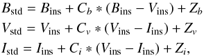$\begin{array}{ccc}& & {\mathit{B}}_{\mathrm{std}}\mathrm{=}{\mathit{B}}_{\mathrm{ins}}\mathrm{+}{\mathit{C}}_{\mathit{b}}\mathrm{\ast }\mathrm{(}{\mathit{B}}_{\mathrm{ins}}\mathrm{-}{\mathit{V}}_{\mathrm{ins}}\mathrm{)}\mathrm{+}{\mathit{Z}}_{\mathit{b}}\\ & & {\mathit{V}}_{\mathrm{std}}\mathrm{=}{\mathit{V}}_{\mathrm{ins}}\mathrm{+}{\mathit{C}}_{\mathit{v}}\mathrm{\ast }\mathrm{(}{\mathit{V}}_{\mathrm{ins}}\mathrm{-}{\mathit{I}}_{\mathrm{ins}}\mathrm{)}\mathrm{+}{\mathit{Z}}_{\mathit{v}}\\ & & {\mathit{I}}_{\mathrm{std}}\mathrm{=}{\mathit{I}}_{\mathrm{ins}}\mathrm{+}{\mathit{C}}_{\mathit{i}}\mathrm{\ast }\mathrm{(}{\mathit{V}}_{\mathrm{ins}}\mathrm{-}{\mathit{I}}_{\mathrm{ins}}\mathrm{)}\mathrm{+}{\mathit{Z}}_{\mathit{i}}\mathit{,}\end{array}$where instrumental magnitudes and secondary standard magnitudes are shown by the subscripts “ins” and “std”, respectively. In these equations, C_b,C_v, and C_i are the color terms, while Z_b,Z_v, and Z_i are the global zero-points. The values of the color terms in the present study are 0.40, −0.05, and 0.11 and the zero-points are 24.43, 23.45, and 22.94 for the B, V, and I filters, respectively. The present values of color terms and zero-points are consistent with those posted on the WFI webpage⁴.

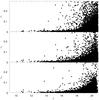Fig. 1 Residual rms around the mean magnitudes in B,V, and I plotted as a function of V magnitude.

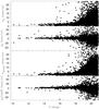Fig. 2 Proper motions and their standard deviations of the mean versus visual magnitude in mas yr-1.

The photometric errors (standard deviations) were calculated by reducing multiple observations to a common reference frame for each particular bandpass. The rms of the residuals around the mean magnitudes for B,V, and I magnitudes are plotted as a function of V magnitude in Fig. 1. The average rms values are better than ~0.01 mag for stars brighter than 18 mag for the B and V filters and better than ~0.02 mag for the I filter.

3. Proper motion determinations

The geometric distortion solution has the smallest residuals for the V filter (Paper I). Additionally, using this filter also reduces color-dependence in our PM analysis. Therefore, we only used V filter images to compute the PMs. A total of two images in the first epoch and four images in the second epoch were used to determine PMs.

A set of probable cluster members was initially selected using the V versus (B − V) CMD. The selected stars lie on the cluster sequences in the CMD and have a magnitude range of 14 ≤ V ≤ 19.0 and are used as a local reference frame to transform the coordinates of the stars between the epochs. By considering only the stars lying on the cluster sequences and having PM errors <5.0 mas yr^-1, we ensured that the proper motions were computed with respect to the bulk motion of the cluster. We used the local transformation approach based on the closest 25 reference stars on the same CCD chip to minimize the influence of uncorrected distortion residuals. No systematics larger than random errors were visible close to the corners or edges of the chips.

Some stars with proper motions that were clearly inconsistent with cluster membership were iteratively removed from the preliminary photometric member list, even though their colors placed them near the fiducial cluster sequence. Figure 2 represents the PMs and their rms errors distributed as a function of V magnitude. The median precision of proper motion measurement is ~2 mas yr^-1 for stars brighter than V = 18 mag. The median value of errors increases up to ~5 mas yr^-1 for stars with V ~ 20 mag. Pryor & Meylan (1993) derived the value of radial velocity dispersion for NGC 6366 as 1.3 km s^-1. Adopting the distance value of the cluster as 3.5 kpc (Harris 1996, 2010 edition), the internal PM dispersion becomes ~0.08 mas yr^-1. This is more than a factor of 20 smaller than our errors, so it is clear that we cannot use our PM measurements for internal dynamics.

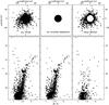Fig. 3 Top panels: proper motion vector-point diagram (VPD). Zero point in VPD is the mean motion of cluster stars. Bottom panels: calibrated V vs. (B − V) CMD. Left: the entire sample; center: stars in VPD within 7.5 mas yr-1 around the cluster mean; right: probable background/foreground field stars in the area of NGC 6366. All plots show only stars with proper motion σ smaller than ~7.5 mas yr-1 in each coordinate.

3.1. Cluster CMD decontamination

One of the strengths of proper motions is to separate out the field stars from the cluster sample and to produce a CMD with only the most likely cluster stars. In Fig. 3 we show how effectively the proper motions separate the field stars by using vector-point diagrams (VPDs) in the top panels, in combination with V versus (B − V) CMDs in the bottom panels. The left panels show the whole sample of stars, while the middle and right panels show probable cluster members and field stars, respectively. The VPD in the middle panel has a circle of radius ~7.5 mas yr^-1 around the cluster centroid, which is provisionally our criterion for discriminating between members (inside) and field stars (outside) and is used before we determine the membership probabilities. This adopted radius is a compromise between losing cluster members with poorly measured PMs and including the field stars sharing the PMs with cluster mean PM. The shape of the cluster members’ PM is round, which indicates that our PM measurements are not affected by any systematics. As can be seen in the figure, the separation of field stars is not clearly visible for the stars fainter than 18.5 mag. In a nutshell, we conclude that PMs for the fainter stars have not been determined accurately.

The UCAC4 catalogue (Zacharias et al. 2013) lists the absolute proper motions of stars in the region of NGC 6366. We found 215 common stars with the UCAC4 catalogue brighter than V = 17 mag. To compare our PMs with UCAC4, we changed the UCAC4 PMs to relative proper motions by subtracting the median PM value of UCAC4 stars (μ_αcosδ = −1.3 mas yr^-1, μ_δ = −1.0 mas yr^-1) from the individual PMs of UCAC4. The results of the comparison are shown in Fig. 4. The top left panel in the figure shows the VPD of UCAC4 stars, while the top right panel shows the VPD of the present measurements. In both the VPDs, a concentration of stars can be seen around (0, 0) mas yr^-1. Our proper motions distribution is tighter than the UCAC4 distribution. This shows that our data is more precise than the UCAC4 data. The 3σ clipped median of the X and Y PM differences plotted in the bottom panel of Fig. 4 are 0.5 mas yr^-1 and −0.3 mas yr^-1. Clearly, our measurements are consistent with the UCAC4 data for V ≤ 17 mag.

4. Membership probabilities

In Fig. 3, two distinct group of stars are clearly visible, the majority of them belonging to the cluster. Determination of the membership probabilities is a very important step for further studies of the cluster using only the most probable cluster members. The pioneering work by Vasilevskis et al. (1958) set up the fundamental mathematical model for membership determination. Sanders (1971) used maximum-likelihood principles for computing membership probabilities. Since then, the methods used to determine the membership have been continuously refined (Stetson 1980; Zhao & He 1990; Zhao & Shao 1994). In the present work, we followed the method described in Balaguer-Núñez et al. (1998). This is the same method that we used for NGC 6809 (Sariya et al. 2012) and NGC 3766 (Yadav et al. 2013). According to this method, the frequency distribution functions of cluster stars (${\mathit{\phi }}_{\mathrm{c}}^{\mathit{\nu }}$) and field stars (${\mathit{\phi }}_{\mathrm{f}}^{\mathit{\nu }}$) are constructed for the ith star using the equations $\begin{array}{ccc}{\mathit{\phi }}_{\mathrm{c}}^{\mathit{\nu }}& \mathrm{=}& \frac{\mathrm{1}}{\mathrm{2}\mathit{\pi }\sqrt{\mathrm{(}{\mathit{\sigma }}_{\mathrm{c}}^{\mathrm{2}}\mathrm{+}{\mathit{ϵ}}_{\mathit{xi}}^{\mathrm{2}}\mathrm{)}\mathrm{(}{\mathit{\sigma }}_{\mathrm{c}}^{\mathrm{2}}\mathrm{+}{\mathit{ϵ}}_{\mathit{yi}}^{\mathrm{2}}\mathrm{)}}}\\ & & \mathrm{\times }\exp \begin{array}{c}\mathrm{⎧}\\ \mathrm{⎪}\\ \mathrm{⎪}\\ \mathrm{⎨}\\ \mathrm{⎪}\\ \mathrm{⎪}\\ \mathrm{⎩}\end{array}\mathrm{-}\frac{\mathrm{1}}{\mathrm{2}}\left[\frac{\mathrm{(}{\mathit{\mu }}_{\mathit{xi}}\mathrm{-}{\mathit{\mu }}_{\mathit{xc}}{\mathrm{)}}^{\mathrm{2}}}{{\mathit{\sigma }}_{\mathrm{c}}^{\mathrm{2}}\mathrm{+}{\mathit{ϵ}}_{\mathit{xi}}^{\mathrm{2}}}\mathrm{+}\frac{\mathrm{(}{\mathit{\mu }}_{\mathit{yi}}\mathrm{-}{\mathit{\mu }}_{\mathit{yc}}{\mathrm{)}}^{\mathrm{2}}}{{\mathit{\sigma }}_{\mathrm{c}}^{\mathrm{2}}\mathrm{+}{\mathit{ϵ}}_{\mathit{yi}}^{\mathrm{2}}}\right]\begin{array}{c}\mathrm{⎫}\\ \mathrm{⎪}\\ \mathrm{⎪}\\ \mathrm{⎬}\\ \mathrm{⎪}\\ \mathrm{⎪}\\ \mathrm{⎭}\end{array}\end{array}$and $\begin{array}{ccc}{\mathit{\phi }}_{\mathrm{f}}^{\mathit{\nu }}& \mathrm{=}& \frac{\mathrm{1}}{\mathrm{2}\mathit{\pi }\sqrt{\mathrm{(}\mathrm{1}\mathrm{-}{\mathit{\gamma }}^{\mathrm{2}}\mathrm{)}}\sqrt{\mathrm{(}{\mathit{\sigma }}_{\mathit{x}\mathrm{f}}^{\mathrm{2}}\mathrm{+}{\mathit{ϵ}}_{\mathit{xi}}^{\mathrm{2}}\mathrm{)}\mathrm{(}{\mathit{\sigma }}_{\mathit{y}\mathrm{f}}^{\mathrm{2}}\mathrm{+}{\mathit{ϵ}}_{\mathit{yi}}^{\mathrm{2}}\mathrm{)}}}\\ & & \mathrm{\times }\exp \{\mathrm{-}\frac{\mathrm{1}}{\mathrm{2}\mathrm{(}\mathrm{1}\mathrm{-}{\mathit{\gamma }}^{\mathrm{2}}\mathrm{)}}[\frac{\mathrm{(}{\mathit{\mu }}_{\mathit{xi}}\mathrm{-}{\mathit{\mu }}_{\mathit{x}\mathrm{f}}{\mathrm{)}}^{\mathrm{2}}}{{\mathit{\sigma }}_{\mathit{x}\mathrm{f}}^{\mathrm{2}}\mathrm{+}{\mathit{ϵ}}_{\mathit{xi}}^{\mathrm{2}}}\\ & & \mathrm{-}\frac{\mathrm{2}\mathit{\gamma }\mathrm{(}{\mathit{\mu }}_{\mathit{xi}}\mathrm{-}{\mathit{\mu }}_{\mathit{x}\mathrm{f}}\mathrm{)}\mathrm{(}{\mathit{\mu }}_{\mathit{yi}}\mathrm{-}{\mathit{\mu }}_{\mathit{y}\mathrm{f}}\mathrm{)}}{\sqrt{\mathrm{(}{\mathit{\sigma }}_{\mathit{x}\mathrm{f}}^{\mathrm{2}}\mathrm{+}{\mathit{ϵ}}_{\mathit{xi}}^{\mathrm{2}}\mathrm{)}\mathrm{(}{\mathit{\sigma }}_{\mathit{y}\mathrm{f}}^{\mathrm{2}}\mathrm{+}{\mathit{ϵ}}_{\mathit{yi}}^{\mathrm{2}}\mathrm{)}}}\mathrm{+}\frac{\mathrm{(}{\mathit{\mu }}_{\mathit{yi}}\mathrm{-}{\mathit{\mu }}_{\mathit{y}\mathrm{f}}{\mathrm{)}}^{\mathrm{2}}}{{\mathit{\sigma }}_{\mathit{y}\mathrm{f}}^{\mathrm{2}}\mathrm{+}{\mathit{ϵ}}_{\mathit{yi}}^{\mathrm{2}}}]\begin{array}{c}\mathrm{⎫}\\ \mathrm{⎪}\\ \mathrm{⎪}\\ \mathrm{⎪}\\ \mathrm{⎪}\\ \mathrm{⎬}\\ \mathrm{⎪}\\ \mathrm{⎪}\\ \mathrm{⎪}\\ \mathrm{⎪}\\ \mathrm{⎭}\end{array}\end{array}$where (μ_xi, μ_yi) are the proper motions of the ith star, while (ϵ_xi, ϵ_yi) are the observed errors in proper motions components. The parameters μ_xc and μ_yc are the cluster’s proper motion center and μ_xf and μ_yf are the field proper motion center; σ_c is the intrinsic proper motion dispersion of cluster member stars, whereas σ_xf and σ_yf are the field intrinsic proper motion dispersions; and γ is the correlation coefficient calculated by $\begin{array}{ccc}\mathit{\gamma }\mathrm{=}\frac{\mathrm{(}{\mathit{\mu }}_{\mathit{xi}}\mathrm{-}{\mathit{\mu }}_{\mathit{x}\mathrm{f}}\mathrm{)}\mathrm{(}{\mathit{\mu }}_{\mathit{yi}}\mathrm{-}{\mathit{\mu }}_{\mathit{y}\mathrm{f}}\mathrm{)}}{{\mathit{\sigma }}_{\mathit{x}\mathrm{f}}{\mathit{\sigma }}_{\mathit{y}\mathrm{f}}}\mathrm{·}& & \end{array}$(1)Because the observed field is small, we did not consider the spatial distribution of the stars. The stars used to calculate ${\mathit{\phi }}_{\mathrm{c}}^{\mathit{\nu }}$ and ${\mathit{\phi }}_{\mathrm{f}}^{\mathit{\nu }}$ have PM errors better than 7.5 mas yr^-1. Consistent with the relative nature of our PMs, the center of the stars in VPD is found to be (μ_xc, μ_yc) = (0, 0) mas yr^-1. As mentioned above, given our errors we do not anticipate being able to measure the internal dispersion of PMs for the cluster stars (σ_c), hence we used σ_c = 0.08 mas yr^-1 as calculated in Sect. 3. For field stars, we have μ_xf = −9.6 mas yr^-1, μ_yf = −11.1 mas yr^-1, σ_xf = 6.8 mas yr^-1, and σ_yf = 4.8 mas yr^-1.

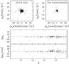Fig. 4 Top panels: vector-point diagrams of common stars relative to the cluster mean motion for UCAC4 (left) and our measurements (right). Bottom panels: right ascension (bottom) and declination (top) proper motion differences as a function of V magnitude between UCAC4 and our measurements. Horizontal dashed lines show the 3σ-clipped median of the proper motion difference between UCAC4 and our data.

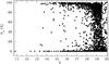Fig. 5 Membership probability Pμ(%) as a function of V magnitude. At V ~ 18.5 mag and fainter, Pμ decreases as a result of increasing errors in the PMs.

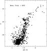Fig. 6 Color–magnitude diagram for the stars with membership probability >80%

The total distribution function can be computed as $\begin{array}{ccc}\mathit{\phi }\mathrm{=}\mathrm{(}{\mathit{n}}_{\mathrm{c}}\mathit{.}{\mathit{\phi }}_{\mathrm{c}}^{\mathit{\nu }}\mathrm{)}\mathrm{+}\mathrm{(}{\mathit{n}}_{\mathrm{f}}\mathit{.}{\mathit{\phi }}_{\mathrm{f}}^{\mathit{\nu }}\mathrm{)}\mathit{,}& & \end{array}$(2)where n_c and n_f are the normalized number of stars for cluster and field (n_c + n_f = 1). Therefore, the membership probability for the ith star is $\begin{array}{ccc}{\mathit{P}}_{\mathit{\mu }}\mathrm{\left(}\mathit{i}\mathrm{\right)}\mathrm{=}\frac{{\mathit{\phi }}_{\mathrm{c}}\mathrm{\left(}\mathit{i}\mathrm{\right)}}{\mathit{\phi }\mathrm{\left(}\mathit{i}\mathrm{\right)}}\mathrm{·}& & \end{array}$(3)The membership probability is a good indicator of how well we can discriminate between cluster and field stars. In Fig. 5, membership probability has been plotted as a function of V magnitude. In this figure, clear separation of cluster and field stars can be observed as a sharp distribution of stars near membership values P_μ ~ 100% and P_μ ~ 0%. There is an increase in the number of stars with intermediate values of P_μ, for stars fainter than V = 18.5 mag as a result of increasing measurement errors.

In Fig. 6, stars with P_μ> 80% are shown in the CMD. This CMD exhibits cluster sequences down to V ~ 19.5 mag and distinct population of subgiants, red giants, horizontal branch stars and blue stragglers. The broadening of the sequences in the CMD is due to the high reddening in the direction of NGC 6366. It can also be seen that the cluster shows a red horizontal branch, which is a signature of metal-rich globular clusters.

5. Applications

5.1. Membership of variables and X-ray sources

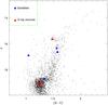Fig. 7 Color−magnitude diagram for the stars whose membership probabilities have been calculated. The variable stars and X-ray sources listed in Table 3 are shown with different symbols indicated in the inset.

We have used our catalogue to check the membership status for the known variables and X-ray sources in the cluster region. Bassa et al. (2008) present 14 X-ray sources in the direction of NGC 6366, 5 of which (CX01-CX05) are located within the half-mass radius of the cluster, while the remaining sources (CX06-CX14) lie outside the half-mass radius. As can be seen in Table 3, four of the sources (CX02, CX08, CX13, CX14) have P_μ ~ 0%, so they are non-members according to our study. The X-ray source CX05 is most probably a cluster member, while the probability that CX07 is a cluster member is very low.

The variable stars in the region of NGC 6366 are listed on Clement’s webpage⁵ of the catalogue of variable stars in globular clusters. Out of the eight variable stars listed on the above webpage, we found four stars in common with our membership catalogue. It is obvious from Table 3 that two variable stars, V5 and V6, are non-members (P_μ = 0%), while V4 and V8 are likely members of NGC 6366. All the X-ray sources and variables discussed above have been plotted in the CMD with different symbols in Fig. 7.

6. The catalogue

Our catalogue presents relative PMs and their errors; membership probabilities; and B,V,I photometric magnitudes with rms errors for 2530 stars in the region of NGC 6366. In the catalogue, Col. (1) provides the running number; Cols. (2) and (3) show the J2000.0 equatorial coordinates, while Cols. (4) and (5) provide the pixel coordinates X and Y. Columns (6) to (9) contain relative proper motions and their standard errors. Columns (10) to (15) present photometric data, i.e., B,V, and I magnitudes and their corresponding errors. If photometry in a specific band is not available, the magnitude is arbitrarily set to 99.9999 with an error of 0.9999. Column (16) gives the membership probability P_μ. The pixel coordinates in reference image are plotted in Fig. 8. The first few lines of the catalogue are shown in Table 4.

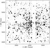Fig. 8 X,Y WFI pixel coordinates in the reference image.

7. Conclusions

The present study has produced a catalogue of stars in NGC 6366 with B,V, and I photometry; proper motions; and membership probabilities. Using our proper motions, we have separated field stars from the cluster members in CMD. The membership catalogue for stars brighter than V ~ 20 mag has been made available to the astronomical community. Our catalogue has been used to provide the membership status for several known variable stars and X-ray sources in the cluster region. We also demonstrate that CCD observations taken just a few years apart can provide precise proper motions.

Acknowledgments

We thank an anonymous referee for a careful reading of the manuscript and for many useful and constructive suggestions. The authors are also grateful to Dr. Fabíola Campos for providing their photometric data for magnitude calibration purpose. This research used the facilities of the Canadian Astronomy Data Centre operated by the National Research Council of Canada with the support of the Canadian Space Agency. We have also used the catalogue of variable stars managed by Prof. Christine Clement from University of Toronto, Canada.

References

All Tables

All Figures

	Fig. 1 Residual rms around the mean magnitudes in B,V, and I plotted as a function of V magnitude.
In the text

	Fig. 2 Proper motions and their standard deviations of the mean versus visual magnitude in mas yr-1.
In the text

Fig. 3 Top panels: proper motion vector-point diagram (VPD). Zero point in VPD is the mean motion of cluster stars. Bottom panels: calibrated V vs. (B − V) CMD. Left: the entire sample; center: stars in VPD within 7.5 mas yr-1 around the cluster mean; right: probable background/foreground field stars in the area of NGC 6366. All plots show only stars with proper motion σ smaller than ~7.5 mas yr-1 in each coordinate.

In the text

Fig. 4 Top panels: vector-point diagrams of common stars relative to the cluster mean motion for UCAC4 (left) and our measurements (right). Bottom panels: right ascension (bottom) and declination (top) proper motion differences as a function of V magnitude between UCAC4 and our measurements. Horizontal dashed lines show the 3σ-clipped median of the proper motion difference between UCAC4 and our data.

In the text

	Fig. 5 Membership probability Pμ(%) as a function of V magnitude. At V ~ 18.5 mag and fainter, Pμ decreases as a result of increasing errors in the PMs.
In the text

	Fig. 6 Color–magnitude diagram for the stars with membership probability >80%
In the text

	Fig. 7 Color−magnitude diagram for the stars whose membership probabilities have been calculated. The variable stars and X-ray sources listed in Table 3 are shown with different symbols indicated in the inset.
In the text

	Fig. 8 X,Y WFI pixel coordinates in the reference image.
In the text

References

- Alonso, A., Salaris, M., Martínez-Roger, C., Straniero, O., & Arribas, S. 1997, A&A, 323, 374 [NASA ADS] [Google Scholar]
- Anderson, J., Bedin, L. R., Piotto, G., Yadav, R. K. S., & Bellini, A. 2006, A&A, 454, 1029 (Paper I) [NASA ADS] [CrossRef] [EDP Sciences] [Google Scholar]
- Arellano Ferro, A., Giridhar, S., Rojas Lopez, V., et al. 2008, Rev. Mex. Astron. Astrofis., 44, 365 [NASA ADS] [Google Scholar]
- Armandroff, T. E. 1989, AJ, 97, 375 [NASA ADS] [CrossRef] [Google Scholar]
- Balaguer-Núñez, L., Tian, K. P., & Zhao, J. L. 1998, A&AS, 133, 387 [NASA ADS] [CrossRef] [EDP Sciences] [Google Scholar]
- Bassa, C. G., Pooley, D., Verbunt, F., et al. 2008, A&A, 488, 921 [NASA ADS] [CrossRef] [EDP Sciences] [Google Scholar]
- Bellini, A., Piotto, G., Bedin, L. R., et al. 2009, A&A, 493, 959 [NASA ADS] [CrossRef] [EDP Sciences] [Google Scholar]
- Campos, F., Kepler, S. O., Bonatto, C., & Ducati, J. R. 2013, MNRAS, 433, 243 [NASA ADS] [CrossRef] [Google Scholar]
- Chen, C. W., & Chen, W. P. 2010, ApJ, 721, 1790 [NASA ADS] [CrossRef] [Google Scholar]
- Cudworth, K. M. 1986, IAU Symp., 109, 201 [NASA ADS] [Google Scholar]
- Cudworth, K. M. 1997, ASP Conf. Ser., 127, 91 [NASA ADS] [Google Scholar]
- Da Costa, G. S., & Seitzer, P. 1989, AJ, 97, 405 [NASA ADS] [CrossRef] [Google Scholar]
- Dambis, A. K. 2006, Astron. Astrophys. Trans., 25, 185 [NASA ADS] [CrossRef] [Google Scholar]
- Goldsbury, R., Richer, H. B., Anderson, J., et al. 2010, AJ, 140, 1830 [NASA ADS] [CrossRef] [Google Scholar]
- Goldsbury, R., Richer, H. B., Anderson, J., et al. 2011, AJ, 142, 66 [NASA ADS] [CrossRef] [Google Scholar]
- Harris, H. C. 1993, AJ, 106, 604 [NASA ADS] [CrossRef] [Google Scholar]
- Harris, W. E. 1996, AJ, 112, 1487 [NASA ADS] [CrossRef] [Google Scholar]
- Johnston, H. M., Verbunt, F., & Hasinger, G. 1996, A&A, 309, 116 [NASA ADS] [Google Scholar]
- Lloyd, C., Pike, C. D., Terzan, A., & Sawyer Hogg, H. B. 2008, The Observatory, 128, 280 [NASA ADS] [Google Scholar]
- Mould, J., Stutman, D., & McElroy, D. 1979, ApJ, 228, 423 [NASA ADS] [CrossRef] [Google Scholar]
- Paust, N. E. Q., Aparicio, A., Piotto, G., et al. 2009, AJ, 137, 246 [NASA ADS] [CrossRef] [Google Scholar]
- Pike, C. D. 1976, MNRAS, 177, 257 [NASA ADS] [CrossRef] [Google Scholar]
- Pryor, C., & Meylan, G. 1993, ASP Conf. Ser., 50, 357 [Google Scholar]
- Sagar, R., & Bhatt, H. C. 1989, MNRAS, 236, 865 [NASA ADS] [CrossRef] [Google Scholar]
- Sanders, W. L. 1971, A&A, 14, 226 [NASA ADS] [Google Scholar]
- Sariya, D. P., Yadav, R. K. S., & Bellini, A. 2012, A&A, 543, A87 [NASA ADS] [CrossRef] [EDP Sciences] [Google Scholar]
- Sawyer, H. B. 1940, Publ. David Dunlap Obs., 1, 179 [NASA ADS] [Google Scholar]
- Stetson, P. B. 1980, AJ, 85, 387 [NASA ADS] [CrossRef] [Google Scholar]
- Thompson, T. A. 2013, MNRAS, 431, 63 [NASA ADS] [CrossRef] [Google Scholar]
- Vasilevskis, S., Klemola, A., & Preston, G. 1958, AJ, 63, 387 [NASA ADS] [CrossRef] [Google Scholar]
- Webbink, R. F. 1985, Dynamics of star clusters, IAU Symp., 113, 541 [Google Scholar]
- Yadav, R. K. S., Bedin, L. R., Piotto, G., et al. 2008, A&A, 484, 609 [NASA ADS] [CrossRef] [EDP Sciences] [Google Scholar]
- Yadav, R. K. S., Sariya, D. P., & Sagar, R. 2013, MNRAS, 430, 3350 [NASA ADS] [CrossRef] [Google Scholar]
- Zacharias, N., Finch, C. T., Girard, T. M., et al. 2013, AJ, 145, 44 [NASA ADS] [CrossRef] [EDP Sciences] [Google Scholar]
- Zhao, J. L., & He, Y. P. 1990, A&A, 237, 54 [NASA ADS] [Google Scholar]
- Zhao, J. L., & Shao, Z. Y. 1994, A&A, 288, 89 [NASA ADS] [Google Scholar]
- Zinn, R. 1985, ApJ, 293, 424 [Google Scholar]