| Issue |
A&A
Volume 583, November 2015
|
|
|---|---|---|
| Article Number | A86 | |
| Number of page(s) | 9 | |
| Section | Stellar atmospheres | |
| DOI | https://doi.org/10.1051/0004-6361/201527169 | |
| Published online | 30 October 2015 | |
DB white dwarfs in the Sloan Digital Sky Survey data release 10 and 12⋆
1 Institut für Theoretische Physik und Astrophysik, Universität Kiel, 24098 Kiel, Germany
e-mail: This email address is being protected from spambots. You need JavaScript enabled to view it.
2 Instituto de Fisica, Universidade Federal do Rio Grande do Sul, 91501-900 Porto-Alegre, RS, Brazil
Received: 11 August 2015
Accepted: 26 August 2015
Abstract
Aims. White dwarfs with helium-dominated atmospheres (spectral types DO, DB) comprise approximately 20% of all white dwarfs. There are fewer studies than of their hydrogen-rich counterparts (DA) and thus several questions remain open. Among these are the total masses and the origin of the hydrogen traces observed in a large number and the nature of the deficit of DBs in the range from 30 000−45 000 K. We use the largest-ever sample (by a factor of 10) provided by the Sloan Digital Sky Survey (SDSS) to study these questions.
Methods. The photometric and spectroscopic data of 1107 helium-rich objects from the SDSS are analyzed using theoretical model atmospheres. Along with the effective temperature and surface gravity, we also determine hydrogen and calcium abundances or upper limits for all objects. The atmosphere models are extended with envelope calculations to determine the extent of the helium convection zones and thus the total amount of hydrogen and calcium present.
Results. When accounting for problems in determining surface gravities at low Teff , we find an average mass for helium-dominated white dwarfs of 0.606 ± 0.004 M⊙, which is very similar to the latest determinations for DAs. There are 32% of the sample with detected hydrogen, but this increases to 75% if only the objects with the highest signal-to-noise ratios are considered. In addition, 10−12% show traces of calcium, which must come from an external source. The interstellar medium (ISM) is ruled out by the fact that all polluted objects show a Ca/H ratio that is much larger than solar. We also present arguments that demonstrate that the hydrogen is very likely not accreted from the ISM but is the result of convective mixing of a residual thin hydrogen layer with the developing helium convection zone. It is very important to carefully consider the bias from observational selection effects when drawing these conclusions.
Key words: white dwarfs / stars: atmospheres / stars: abundances / convection / accretion, accretion disks
Table 1 is only available at the CDS via anonymous ftp to cdsarc.u-strasbg.fr (130.79.128.5) or via http://cdsarc.u-strasbg.fr/viz-bin/qcat?J/A+A/583/A86
© ESO, 2015
1. Introduction
Approximately 20% of all white dwarfs have atmospheres dominated by helium. Above Teff≈ 40 000 K, He ii lines are strong and the stars are classified as spectral type DO or DOA if, in addition, Balmer lines of hydrogen are visible, or as DAO if these are dominant. Below this temperature He i lines are dominant and the spectral type is DB. If traces of other elements are present, more letters are added to the type, e.g., A for hydrogen, Z for metals (Sion et al. 1983). The existence of almost pure hydrogen (DA) and almost pure helium atmospheres as a result of gravitational settling is well understood, with the lightest element present floating to the top of the outer layers (Schatzman 1948). Helium-rich white dwarfs must have almost completely lost their outer hydrogen layer in a previous evolutionary phase; the currently accepted scenario is the born again or late thermal pulse scenario (Iben et al. 1983).
Questions remain as to the so-called DB gap and the origin of hydrogen traces in a large number, perhaps the majority, of DB white dwarfs. The deficit of DBs between 30 000 and 45 000 K was first identified by Liebert et al. (1986) and explained in terms of diffusion and convective mixing by Fontaine & Wesemael (1987). Eisenstein et al. (2006) and Kleinman et al. (2013) found several objects within the gap, but the number was still smaller than expected from the simple cooling rates without changes of spectral types. In principle, the observed traces of hydrogen could be explained by two competing theories: accretion of interstellar medium (ISM) or convective mixing with a (thin) hydrogen layer left over from the previous evolution (which, at the same time, could also explain the DB gap).
Two recent studies have analyzed large samples of helium-rich white dwarfs. Voss et al. (2007) used data for 71 objects from the Supernova Ia Progenitor Survey (SPY, Napiwotzki et al. 2003). The typical resolution (depending on the seeing) was ~0.4 Å, with the signal-to-noise ratio (S/N) varying but > 15. The study by Bergeron et al. (2011, henceforth BW11) is the largest so far with 108 objects. The resolution from two different spectrographs was 3−6 Å, with the S/N mostly above 50. In this work we use a sample of 1107 DB (and DBA or DBZ) stars, thus increasing the sample more than tenfold the largest previous ones. The resolution is ~2.5 Å, the S/N ranges from 10 to 75 with an average of 20. The average quality of the spectra is inferior to the BW11 sample in S/N and in resolution to the SPY sample. However, this is compensated for by the huge size and homogeneity, which allows us to study statistical properties of the helium-rich white dwarfs with unprecedented quality.
2. The sample
Data release 7 (DR7, Kleinman et al. 2013) of the Sloan Digital Sky Survey (SDSS) contained spectra of 923 stars classified as DB (helium atmospheres). DR10 (Kepler et al. 2015b) added another 450 (including subtypes DBA with hydrogen traces and DBZ with metals), and DR12 (Kepler et al. 2015a) added 121 more, all of which are new detections. The number of spectra is larger since several have two or three spectra in the database. From this database we first selected all those with S/N greater than 10.
After a first tentative fit with model spectra (see below for details) and a visual inspection we eliminated all objects with peculiarities, such as a red unresolved companion (DB+dM), presence of He ii lines (DO), obvious magnetic splitting of spectral lines, very marginal or invisible He lines (DC), or spectra with strong artifacts. We did not eliminate DB stars with traces of hydrogen (DBA) or calcium H+K lines (DBZ). This left us with a sample of 1267 spectra of 1107 different objects, of which 13 had three and 136 had two spectra. In addition to the spectra, we used the SDSS photometry, available for each object in the sample.
3. Atmospheric parameters
Atmospheric parameters Teff , log g , abundances, or upper limits of hydrogen and calcium were determined by a comparison of observations with several grids of theoretical model atmospheres. The input physics and procedures used are described in Koester (2010). We use the mixing-length approximation for convection in the version ML2 (Fontaine et al. 1981; Tassoul et al. 1990) with a mixing length equal to 1.25 pressure scale heights. A pure helium grid – for technical reasons the logarithmic abundance ratio of hydrogen to helium, log NH/NHe (abbreviated [H/He] henceforth) is −20.0 – covers effective temperatures from 10 000 to 50 000 K, with step widths ranging from 250 to 500 K from low to high effective temperatures. The surface gravity log g ranged from 6.00 to 9.50, with step width 0.25. In addition to the pure helium grid above, we also calculated grids with various [H/He] ratios: −6.0, −5.5, −5.0, −4.5, −4.0, −3.5, and −3.0. These grids covered the same Teff and log g values, except that the log g range only covered from 7.0 to 9.0. Details of the analysis are described in the following.
3.1. Photometry
From the synthetic spectra we calculated theoretical photometry in the SDSS system. The effect of the surface gravity on the photometry is small; in the first step of the fitting procedure, we thus kept this parameter fixed at the canonical value of 8.0. A possible concern for the fainter objects at greater distance is interstellar reddening, which leads to lower apparent temperatures. We determined three different fit results: one assuming that the reddening is negligible, a second that assumes the maximum reddening from the Schlafly & Finkbeiner (2011) extinction map, and a third value that uses an iterative procedure as described in Tremblay et al. (2011) and Genest-Beaulieu & Bergeron (2014). Basically, this method assumes that the extinction is negligible within 100 pc, and from there it increases linearly to the maximum value at a vertical height z = 250 pc above the Galactic plane. This approach also gives the best approximation for the distance and z, although it should be kept in mind at this step a fixed radius corresponding to log g = 8.0 and a pure He atmosphere is assumed for all objects.
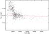 |
Fig. 1 Surface gravity log g as a function of effective temperature. The continuous (red) line is the sequence for a constant mass of 0.6 M⊙. |
3.2. Spectroscopy
As a next step the observed spectra were fitted with the pure He grid, to determine Teff and log g . A well known problem in many cases is that there are two possible solutions corresponding to local χ2 minima, one below and one above the region of Teff = 24 000−26 000 K, where the He lines reach their maximum strength. The χ2 values of the two solutions are usually very similar or even identical and cannot be trusted to select the correct solution. We used the photometric fits, which do not have this problem, as well as visual inspection of all fits, to minimize wrong choices.
Then, in all spectra we used an automatic measuring procedure to determine Hα equivalent widths and uncertainties, or alternatively upper limits; all positive and negative detections were confirmed by visual inspection. These measurements were compared to theoretical equivalent widths from the grids with various hydrogen traces as described above, and hydrogen abundances [H/He], uncertainties, or upper limits were determined. With this additional knowledge, the spectral fits were repeated with the grid that matched to the measured abundance most closely, and this whole procedure was iterated until the parameters were determined with (almost) fully consistent theoretical models. As a final step, the photometric fit was repeated, but now keeping all parameters from the spectroscopic results fixed and solving only for the consistent distance and Galactic position. Table 1 (available at the CDS) contains the final results of this analysis.
Average surface gravity log g as a function of effective temperature Teff in 19 intervals.
4. Analysis
4.1. Surface gravity and masses
Figure 1 shows the surface gravity versus effective temperature for all objects, except for a few low temperature DBs, where the spectroscopic fitting did not converge on a log g within the grid; Table 1 shows more detail in numerical form. Some features of this result are immediately apparent:
-
the log g and masses are significantly higher below 16 000 K than for the hotter objects. This effect has been observed before, e.g., by Kepler et al. (2007), BW11, and Kepler et al. (2015b). BW11 tentatively conclude that the large mass spread might be real for Teff> 13 000 K, given the presence of larger and smaller log g determinations in the same temperature interval and a comparison of spectroscopic and parallax distances of 11 objects. Only one of the 11 objects has a really large spectroscopic mass, and for this one the two distances show a large discrepancy; the authors admit that at these low temperatures the limit of the spectroscopic method may have been reached, because of the weakness of the He lines. We believe that the systematic change in our sample (Fig. 1) is caused by an imperfect implementation of line broadening by neutral helium, which dominates the broadening below 16 000 K.
-
There is also a significant increase in the width of the log g distribution, in addition to this systematic effect. The explanation is most likely the decreasing strength of the helium lines in conjunction with the moderate resolution and S/N of the SDSS spectra, which increase the errors of the individual parameter determinations. Because of these results, we only use the solution with log g fixed at 8.0 for Teff< 16 000 K and assume an error for log g of 0.25.
-
The average mass in Table 2 shows little variation in the range 16 000 ≤ Teff ≤ 22 000 K with an average over this whole range of 0.606 ± 0.004 M⊙. In six of the seven highly populated intervals, the average agrees with this value within the 1σ errors, and in the other within 2σ, which is close to expectation, if the average mass is indeed constant. We conclude that this is a realistic estimate of the average mass of DB (including DBA, DBZ) white dwarfs and that any averaging that includes cooler or hotter objects will necessarily lead to erroneous results. For example, for our complete sample we get an unreliable average of 0.706 ± 0.006 M⊙.
-
DBs at 10 000 K are approximately 5 × 10⁸ yr older than at 30 000 K. They may originate from more massive progenitor stars on the main sequence and end up as higher mass white dwarfs. Using data from Salaris et al. (2009) and Pietrinferni et al. (2004), we estimate that this effect could account for a difference of about 0.05 M⊙ over the observed range. This could explain the slightly lower mass at the high Teff end, but certainly not the large increase below 16 000 K.
-
Both Fig. 1 and Table 2 show a deficiency of objects – almost a gap – in the interval 24 000−26 000 K, in comparison to both neighboring intervals. To demonstrate that such a gap is not expected from evolution or observational effects, we calculated the quantity BR in the last column of the table. This is the number of objects divided by the cooling time during the interval and by the luminosity L3/2, and scaled by an arbitrary constant for easier comparison. The first factor takes the different times spent in each interval during the cooling into account, and the second the larger observation volume for intrinsically brighter objects. If the observations were complete and a magnitude-limited sample, this number would be proportional to the birthrate of DB white dwarfs, and thus be a constant, if all DBs originate at high Teff and only evolve through the range of our sample (see below). Obviously these conditions are not fulfilled; nevertheless, even with these numbers, the gap 24 000−26 000 K is significant. (We note that the apparent gap is centered on 26 000 K, and the argument would be even more convincing had we used the interval 25 000−27 000 K.)
Our explanation of the last point is as follows: this temperature region is exactly where the helium lines have their maximum strength as a function of effective temperature. If the predicted line strengths are greater than attained by the observed objects, then the fitting procedure will force them to a solution on either side of the maximum. BW11 also discuss this possibility and conclude that a mixing-length parameter α = 1.25 (which is also our choice) provides the smoothest distribution of stars over the temperature range. However, because of their smaller sample, there are only ~20 objects between 20 000 and 30 000 K, compared to 134 in our sample. Judging by Fig. 2 in BW11, a slightly larger α would probably give a more plausible distribution for our sample.
An alternative suggestion, made by the referee, is a possible small error in the SDSS flux calibration (see below for further discussion). A possible indication for this is that two of the common objects between the BW11 and our sample have Teff ~26 000 K in BW11, but 24 000 and 28 000 K in our determination.
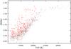 |
Fig. 2 Logarithmic hydrogen abundance [H/He] as a function of Teff . Red circles indicate detected abundances, black symbols indicate upper limits. |
4.2. Hydrogen abundance
The hydrogen abundance as a function of Teff is shown in Fig. 2. The detection limit is high at high temperatures because the hydrogen spectral lines get weaker. On the other hand, at low temperatures, much smaller abundances can easily be detected. The abundances, however, do not reach the same level as at the high Teff end, because the hydrogen gets diluted by the increasing depth of the convection zone. Out of a total of 1036 objects with Teff< 23 000 K, 329 or 32% show hydrogen. However, our sample extends over a large range of S/N values and positions in the Galaxy that have an influence on the observed DBA fraction. This is demonstrated in Table 3.
The S/N is an obvious factor influencing the detectability of hydrogen. The percentage of DBAs increases very significantly with increasing S/N, from 37% for the subsample with z ≤ 250 pc to 75% at the highest S/N. This is even higher than the values of 44% found by BW11 and 55% by Voss et al. (2007), regarded as being lower limits in those papers. Our findings suggest that practically all DBs show some trace of hydrogen if the resolution and S/N are high enough.
With the large size of our sample and the excellent SDSS photometry, for the first time we can try to study the position of DBs and DBAs in the Galaxy, in particular the height above the Galactic plane. This is an important quantity for the question: is the hydrogen content due to external processes, e.g., accretion from interstellar gas, or from the remnants of a planetary system, or to an intrinsic process like dilution of an outer hydrogen envelope in a developing helium convection zone. Figure 3 shows this distribution, which demonstrates a concentration of the DBAs towards the Galactic plane. The effect becomes even clearer in Table 3, which shows a decrease in the DBA percentage with height z. Before jumping to premature conclusions, however, we need to take into account that the group with z> 250 pc has on average larger distances and lower S/N, which possibly alone could explain the z dependence. To test this we have taken a progressively smaller limit on the S/N, to make both groups more comparable. Taking only objects with 10 ≤ S/N ≤ 15, the average S/N and its distribution become almost identical. For this sample the difference between the two groups disappears (last lines in Table 3): taking samples with comparable S/N, there is no obvious concentration toward the Galactic plane.
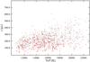 |
Fig. 3 Distribution of DBAs (red circles) and DBs (black crosses) with height z above the Galactic plane. The general decrease of distances towards lower Teff is very likely caused by the lower luminosity of the cooler objects. |
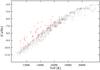 |
Fig. 4 Logarithmic calcium abundance [Ca/He] as a function of Teff . Red circles represent detected abundances, and black symbols the upper limits. |
Dependence of the DBA/(DBA+DB) number ratio on the signal-to-noise (S/N) and position in the Galaxy z.
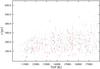 |
Fig. 5 Distribution of DBZs (red circles) and DBs (black limit symbols) with height z above the Galactic plane. |
4.3. Metals in DBs: the DBZs
Seventy-five objects show the H+K resonance lines of ionized calcium – this is the only metal detected in our sample. Figures 4 and 5 and Table 4 show the distribution of the DBZs with Teff , S/N, and z in the same way as for hydrogen in the previous figures and tables. Surprisingly, the fraction of DBZs shows little variation with the S/N, which might even be explainable by the smaller numbers. The only explanation we can find is that the Ca ii lines are much narrower and deeper than Hα, and therefore easier to detect, even at low S/N. The change of the ratio with z is smaller than that for hydrogen (from 11.4 to 8.3%) and even reverses when using the limited sample with S/N between ten and 15. The numbers are still relatively small, but we can definitely state that they do not prove any preference for accretion of ISM close to the Galactic plane (Fig. 5).
4.4. Error estimates
The errors for Teff and log g in Table 2 are only formal statistical errors and thus underestimate the real uncertainties. Fortunately we have multiple spectra for 149 objects, leading to 162 pairs of Teff determinations and 72 for log g (excluding those with fixed 8.0). The average absolute differences are 3.1% for Teff , 0.12 for log g , 0.18 for [H/He], and 0.25 for [Ca/He]. Since the models and fitting procedures are exactly the same, these are uncertainties due to the observations caused, for example, by different S/N or reductions.
There are 27 objects in common with the sample of BW11. If we compare only the 17 DBs with Teff ≥ 16 000 K, where we determine both parameters, the systematic difference for Teff is −1.3%, i.e. our Teff are slightly larger on average. The dispersion is 4.6%, a reasonable number given that our internal uncertainties are already 3.1%. The differences in surface gravity are larger, with a systematic effect of 0.095 dex. In their study of DA white dwarfs, Genest-Beaulieu & Bergeron (2014), Tremblay et al. (2011), and Gianninas et al. (2011) find similar differences between their own spectra and SDSS samples. They conclude that the most likely reason is a small residual calibration error of the SDSS spectra. It is plausible that such an error would also affect the DB spectra. The log g dispersion between the BW11 and our results for log g is 0.073 dex. The larger internal error that we obtained above may be influenced by different S/N values for the multiple spectra of the same object.
5. Results and discussion
The overall features of our DB sample are similar to the results of BW11 and Voss et al. (2007): an apparent increase in the masses toward lower temperatures, mean mass around 0.6 M⊙, several DBs within the so-called DB gap above 30 000 K, and a large number of DBs contaminated with hydrogen abundances [H/He] between −6 and −3. Apparent differences may at least be partly attributed to the tenfold increase of the sample size.
We do not find the apparent dichotomy at the very cool end between normal masses and a few very high masses near 1.2 M⊙, which probably motivated BW11 to exclude only the few objects in this range when determining a mean mass for DBs. In our sample there is clearly a continuous distribution; the increase in masses starts below 16 000 K. Since the convection zone develops near 30 000 K and deepens significantly below 20 000 K, we think that neutral broadening is a more likely explanation than the convection theory, which is thought to be the reason behind a similar effect in the DAs (Tremblay et al. 2013). For the averaging, we thus use the intervals between 16 000 and 22 000 K, with many objects and a constant mass throughout, which results in a lower mean mass of 0.606 ± 0.004 M⊙ compared to 0.671 M⊙ in BW11. The mean masses of Voss et al. (2007) agree approximately with our current result, but since different mixing-length parameters and different intervals for the averaging were used, the comparison is not very meaningful. We emphasize again that, as long as the reason for the log g increase at the low Teff end is not understood, it is very important to only compare mean masses for well-defined Teff intervals. If we use our complete sample, we obtain a mean mass of 0.706 M⊙, which is even higher than the BW11 result. Our preferred result agrees with the most recent determination of 0.603 ± 0.002 for DA white dwarfs from DR12 by Kepler et al. (2015a), but the caveat above also applies to the DA vs. DB comparison.
5.1. Hydrogen
Our result for the highest S/N objects indicates that at least 75% – and perhaps all DBs – show some contamination with hydrogen. The difference between DBs and DBAs is very likely just a question of the quality of the observations and we no longer distinguish the mean masses for the two groups. Since hydrogen lines are detected much more easily at low Teff , the detections and upper limits go down to abundances around −6. High abundances, as found at high Teff , are not detected in this range, although they would be found easily. The obvious reason is the deepening of the convection zone below ~18 000 K, and indeed, if multiplied with the mass in the convection zone, the total hydrogen masses seem to increase towards lower Teff (Fig. 6). As a reminder, all hydrogen originally present or accreted from any source should always stay at the top of the envelope, in this case within the outer helium convection zone. The total hydrogen mass in an object can thus never decrease with time.
Continuous accretion from the ISM could explain such an increase; dividing the hydrogen masses by the cooling age of the white dwarf indicates time-averaged accretion rates of 10-17 to 10-24 M⊙/yr (Fig. 7). The size of these average rates is reasonable (Dupuis et al. 1993), although the huge spread and the increase toward lower temperatures might be difficult to explain. An alternative proposal, the continuous accretion of comets from an Oort cloud (Veras et al. 2014), could also explain such an increase toward older white dwarfs, but this faces the same problems.
To put these results into proper perspective we have to consider the strong observational selection effects apparent in Fig. 2. Transforming the approximate location of the observable lower limits for the detected DBAs into lower limits for the total H mass in the convection zone leads to the continuous red line in Fig. 6; because of the spread in S/N and range in log g , there is a transition region and some objects are still found below our chosen curve. Below the red line we do not expect to find hydrogen in the objects of our sample. The region is of course not empty but filled with DBs with upper limits to the hydrogen mass between 10-16 and 10-12 M⊙, depending on Teff .
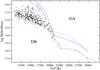 |
Fig. 6 Total hydrogen mass in the convection zone. The continuous red line is the transformed lower limit to the positive detections in Fig. 2. The dotted red curve is the expected location for an abundance [H/He] = –3, which coincides with the continuous red curve at high temperatures. The blue curves indicate the expected hydrogen masses for abundances of −2 (continuous) or −1 (dotted). |
At the hot end all abundances are [H/He] ≈−3.0; we have continued the (theoretical) location for this abundance with the dotted red curve toward lower Teff . Almost all of our objects are confined to the region between these two red curves. Larger abundances are not found, but with our model calculations we can predict their location in Fig. 6. For abundances larger than ~−2 the convection zones in the atmosphere become tiny or absent. Such models are not realistic because the hydrogen would diffuse upward immediately and turn the star into a hydrogen-rich DA – and thus out of our sample. In the upper right part we do not expect to find any DBAs as this region is occupied by DAs. The upper left part also seems sparsely populated. Rare objects like GD16 could fit in there with 11 000 K and log MH/M⊙ ≈ −9 (Koester et al. 2005; Gentile-Fusillo et al., in prep.), but these can easily be misclassified as a DA.
In summary: we find exactly those objects that can exist in our sample, given the observational constraints and the physics of gravitational settling. The morphology of Fig. 7 is very similar to Fig. 6, because the cooling ages change only by 1.5 dex over the whole range of the figure, and the remarks concerning the observable objects are also applicable to the hypothetical accretion rates. The conclusion from this discussion is that Figs. 6 and 7 do not prove that there is any increase in the total hydrogen mass with time. The descendants of the hot DBAs with MH/M⊙ = 10-16 are not the observed cool DBAs but are lost from sight when the H abundance goes below the observable limit. This has to be taken into account when trying to derive conclusions about the origin of hydrogen in DBs from our present results.
Although our approach and presentation are completely different from the theoretical calculations of Macdonald & Vennes (1991), we agree with their prediction that helium-rich DBs with a hydrogen mass > 10-14 M⊙ can only appear below 20 000−22 000 K, depending slightly on the version of the mixing-length theory applied. According to their Fig. 1 and Table 1, higher hydrogen masses appear at progressively lower Teff, where they change from a pure hydrogen object into a DBA (or possibly a DB). If we look closely at the details, however, significant differences appear. To take a specific example: a DA with MH/M⊙ = 10-12 should turn into a DBA only at 11 300 K, whereas we already find such objects around 19 000 K. These problems led BW11 to the hypothesis that hydrogen might not be completely mixed within the He convection zone, but floating only near the top. This would decrease the total amount of H present for a given abundance and effective temperature, thus allowing for a dredge-up at higher Teff . We consider this scenario unlikely since the convection velocities in the highly turbulent convection zone are many orders of magnitude larger than the diffusion velocities of hydrogen in helium. Instead, we prefer to speculate that the discrepancies are due to our imperfect description of convection with the mixing-length theory. Nature somehow seems to manage a complete mixing at 20 000 K, although theory predicts it only happens at 11 300 K.
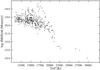 |
Fig. 7 Average rate for the increase in the total hydrogen mass with age of the white dwarf. |
Does this mean that the origin of hydrogen in DBAs is the mixing of a residual small hydrogen layer in the range 30 000−40 000 K, which is left over from the previous evolution? In the framework of interstellar accretion as a source of the hydrogen, one would have to assume a typical average hydrogen accretion rate of 10-19 M⊙/yr for the majority of the cool objects. In 105 yr the star would accumulate an outer H layer of 10-14 M⊙, enough to become a DA. This is a very short time compared to the cooling age at 30 000 K, and for the later evolution it makes no essential difference if the DA arrives with a thin evolutionary H layer or acquires it almost instantaneously through accretion. Both scenarios require that a significant fraction of DA white dwarfs near Teff = 30 000 K have thin hydrogen envelopes in the range of 10-16−10-10 M⊙ . It also requires that many DB/DBA white dwarfs are only borne around 20 000 K and, thus, that their space density, corrected for cooling times (i.e., the luminosity function), is smaller at higher Teff . This is exactly what was found by BW11: the DB to DA ratio of all white dwarfs in the Palomar-Green sample increases sharply around 20 000 K during the cooling sequence.
A decision about the origin of hydrogen then boils down to the question of whether it is more likely for stars to have environments at 30 000 K that lead to accretion rates differing by six orders of magnitude or to have residual hydrogen layers from the previous evolution between 10-16 and 10-10 M⊙. In view of the absence of any correlation between the occurrence of the DBAs and height above the Galactic plane, we favor the second alternative.
As a result of the existence of cool DBs without any visible hydrogen, BW11 concluded that there must be two channels for DBs. One channel consists of DAs that are transformed into DBs through convective mixing, and the other of DBs that never change during evolution. If we accept the view that the hydrogen is residual hydrogen from the previous evolution, then a more natural explanation would be that the hydrogen mass (in DBs) extends from ~ 10-10 M⊙ not just down to 10-16 M⊙, but even lower. The very existence of DBs in the so-called DB gap that exists between 30 000 and 45 000 K proves this. In connection with this it is interesting that the hydrogen layer masses in the ZZ Ceti (DA!) white dwarfs, which are determined by pulsational properties (Romero et al. 2012; Castanheira & Kepler 2009), cover the range from ~ 10-4 to a lower limit of ~ 10-10 M⊙. It is tempting to wonder if we really need two different scenarios for the origin of the hydrogen-rich versus the helium-rich white dwarf sequences or whether we have to accept a continuum of hydrogen layer thickness from the canonical DA value of 10-4 M⊙ down to zero, but such considerations are beyond the scope of this work.
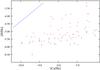 |
Fig. 8 Hydrogen abundance or upper limit versus Ca abundance in all DBZs. The [H/Ca] ratio is smaller than the solar value (continuous line) in all objects. |
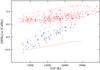 |
Fig. 9 Hydrogen (red circles) and Ca (blue squares) abundance versus Teff. The red dotted line is an empirical upper limit to H abundances, drawn through those objects with the highest abundances. The continuous line is shifted downward by 5.7 dex, the solar H/Ca ratio. Stars with a solar or higher H/Ca would be found below this line, which is, however, below the visibility limit of Ca for all but the coolest stars. |
5.2. Calcium
Unlike hydrogen, calcium does not accumulate in the outer layers with time but diffuses downward with a timescale that is much shorter than the cooling timescale. The origin therefore must be external. If accretion from the ISM (gas and dust) were the source for both hydrogen and calcium, we would thus expect that the Ca/H ratio is always smaller than the solar (ISM) value. On the contrary, Fig. 8 shows the opposite: the ratio in all objects is at least a factor of ten larger than solar. This is a well known fact in many metal-polluted white dwarfs and has always been a problem for the ISM accretion hypothesis. Again, however, selection effects are important in this respect and may lead to wrong conclusions: Fig. 9 demonstrates that there is only a very slim chance of finding such objects at the lowest Teff with the solar ratio in our sample. They must exist, since eventually the calcium will completely diffuse out of the atmosphere, but at this time we cannot find them any more. That we find many objects with Ca is significant and means that, at least in all of these objects, the accretion is currently of extremely hydrogen-poor material. Together with the missing correlation between DBZs and Galactic position, this adds more weight to the hypothesis that ISM accretion cannot explain the observed facts, which leaves the currently favored accretion from a circumstellar dust disk as remnant of a planetary system as the only viable scenario.
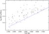 |
Fig. 10 Total calcium mass within the convection zone. The blue continuous line indicates the approximate lower limits, transformed from Fig. 4. |
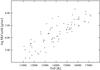 |
Fig. 11 Accretion rate of Ca in g/s, assuming equilibrium between accretion and diffusion. |
The total mass of calcium within the convection zone (Fig. 10) shows the opposite behavior from that of hydrogen – the total amount decreases significantly toward lower temperatures, confirming our assumption that no accumulation occurs with time. It is thus not meaningful to calculate average rates as done for hydrogen, but instead the important timescale for metals would be the diffusion timescale. Assuming equilibrium between diffusion and accretion, we can calculate the calcium accretion flux (Koester 2009). This is presented in Fig. 11, where we have changed the accretion flux unit to g/s, the preferred choice in the case of metal polluted white dwarfs. The lower limit is obtained from the lower limit to the observed abundances in Fig. 4. The strong decline with decreasing Teff is not easy to understand in the currently favored explanation of accretion from a circumstellar disk. If indeed most of the objects are in an equilibrium state between diffusion and accretion, we would expect, on average, constant accretion rates from high to low temperatures, as has been found for metal pollution in DAs (see Fig. 8 in Koester et al. 2014). The problem is already visible in the abundance distribution of Fig. 4; the change of 4.5 orders of magnitude is much more than could be explained by dilution in the He convection zone, which changes only by 1.6 orders over this range. This leads us to ask how accurate our calculations of the convection zone depth are.
5.3. The depth of the helium convection zone
Our envelope code starts at some specific position in the atmosphere model (usually τRoss = 100) and integrates the stellar structure equations inward. The equation of state (EOS) used for hydrogen and helium models is that of Saumon et al. (1995). For a model with Teff = 10 000 K, log g = 8.0 the base of the convection zone is reached at density (g cm-3) log ρ = 2.76 and temperature (K) log T = 6.56. The zone runs through the region of pressure ionization of He (see Fig. 2 of the paper cited above), which is not treated explicitly but bridged by an interpolation scheme. The most important quantity for the envelope structure is the adiabatic gradient, since the convection zone is very nearly adiabatic. Looking at Fig. 23 in Saumon et al. (1995), it is obvious that different EOS give different results for the adiabatic gradient. Considerable scatter is also apparent, which is probably caused by the numerical calculation of second derivatives in the free-energy minimization procedure. As a test of the sensitivity of our envelope structure, we have made a calculation with the adiabatic gradient artificially set to 0.4 everywhere. This decreases the mass in the convection zone by almost three orders of magnitude. While this is certainly an extreme assumption, the extent of the convection zone, and with it the derived total masses of hydrogen and calcium, as well as the diffusion timescales, depend very sensitively on details of the EOS used and could be uncertain by large factors.
6. Conclusions
We analyzed photometry and spectra of the largest sample of helium-rich stars studied so far. The estimated masses show a significant increase below Teff = 16 000 K, which we attributed to imperfect implementation of line broadening by neutral helium atoms. Using the range from 16 000 to 22 000, where the average mass does not change, do we find an average of 0.606 ± 0.004, which is identical to the latest determination for DAs from DR12 (Kepler et al. 2015a).
At least 75% of the helium-rich stars show contamination with hydrogen. The total amount of hydrogen is larger at low Teff than at the hot end. However, we show that when selection effects are taken into account this does not prove that the hydrogen in any single object increases with time. The unavoidable conclusion is that a significant number of DAs must appear at 30 000 K with thin hydrogen layers. Whether (i) these are always ~ 10-16 M⊙ and then increase during evolution by average accretion rates, which have to span the range from 10-23−10-17 M⊙/yr, or whether (ii) the evolutionary hydrogen layer mass spans the range from 10-17−10-10 M⊙ and further accretion is unimportant cannot be distinguished from the current data. Given that there is no correlation of the DBA numbers with distance above the Galactic plane and also that the observed metals cannot be explained by ISM accretion, we prefer the thin H-layer alternative. We admit that the current theoretical calculations predict the existence of stable DBA models with MH from 10-14−10-10 M⊙ between 15 000 and 21 000 K, but not any evolutionary path that would lead there. The solution to this puzzle might be a more physically sound treatment of convection and convective mixing.
About 10−12% of the DBs are contaminated by traces of calcium. This can only be accreted from an external source, and it is very clear that, in all cases, the accreted matter is extremely hydrogen-poor. ISM accretion with solar abundances can be ruled out, and the currently favored model of accretion from a dust disk is supported. If we assume equilibrium between accretion and downward diffusion at the bottom of the convection zone we find calcium accretion rates that decrease strongly with decreasing Teff . We have currently no explanation for this and it might indicate that the extreme physical conditions in the pressure ionization region of helium are not yet adequately described.
Acknowledgments
D.K. gratefully acknowledges support from the program Science without Borders, MCIT/MEC-Brazil, which provided the opportunity for extended visits to Porto Alegre. Funding for SDSS-III has been provided by the Alfred P. Sloan Foundation, the Participating Institutions, the National Science Foundation, and the U.S. Department of Energy Office of Science. The SDSS-III web site is http://www.sdss3.org/. SDSS-III is managed by the Astrophysical Research Consortium for the Participating Institutions of the SDSS-III Collaboration including the University of Arizona, the Brazilian Participation Group, Brookhaven National Laboratory, Carnegie Mellon University, University of Florida, the French Participation Group, the German Participation Group, Harvard University, the Instituto de Astrofisica de Canarias, the Michigan State/Notre Dame/JINA Participation Group, Johns Hopkins University, Lawrence Berkeley National Laboratory, Max Planck Institute for Astrophysics, Max Planck Institute for Extraterrestrial Physics, New Mexico State University, New York University, Ohio State University, Pennsylvania State University, University of Portsmouth, Princeton University, the Spanish Participation Group, University of Tokyo, University of Utah, Vanderbilt University, University of Virginia, University of Washington, and Yale University.
References
- Bergeron, P., Wesemael, F., Dufour, P., et al. 2011, ApJ, 737, 28 [NASA ADS] [CrossRef] [EDP Sciences] [Google Scholar]
- Castanheira, B. G., & Kepler, S. O. 2009, MNRAS, 396, 1709 [NASA ADS] [CrossRef] [Google Scholar]
- Dupuis, J., Fontaine, G., Pelletier, C., & Wesemael, F. 1993, ApJS, 84, 73 [NASA ADS] [CrossRef] [Google Scholar]
- Eisenstein, D. J., Liebert, J., Koester, D., et al. 2006, AJ, 132, 676 [NASA ADS] [CrossRef] [Google Scholar]
- Fontaine, G., & Wesemael, F. 1987, in Conf. Faint Blue Stars, 2nd, Tucson, AZ, June 1–5, 1987, Proc. (A89-17526 05-90), Schenectady, NY, L. Davis Press, Inc., 1987, Discussion, p. 327, 328. NSERC-supported research., 319 [Google Scholar]
- Fontaine, G., Villeneuve, B., & Wilson, J. 1981, ApJ, 243, 550 [NASA ADS] [CrossRef] [Google Scholar]
- Genest-Beaulieu, C., & Bergeron, P. 2014, ApJ, 796, 128 [NASA ADS] [CrossRef] [Google Scholar]
- Gianninas, A., Bergeron, P., & Ruiz, M. T. 2011, ApJ, 743, 138 [NASA ADS] [CrossRef] [Google Scholar]
- Iben, Jr., I., Kaler, J. B., Truran, J. W., & Renzini, A. 1983, ApJ, 264,605 [NASA ADS] [CrossRef] [Google Scholar]
- Kepler, S. O., Kleinman, S. J., Nitta, A., et al. 2007, MNRAS, 375, 1315 [NASA ADS] [CrossRef] [Google Scholar]
- Kepler, S. O. et al. 2015a, MNRAS, submitted [Google Scholar]
- Kepler, S. O., Pelisoli, I., Koester, D., et al. 2015b, MNRAS, 446, 4078 [NASA ADS] [CrossRef] [Google Scholar]
- Kleinman, S. J., Kepler, S. O., Koester, D., et al. 2013, ApJS, 204, 5 [NASA ADS] [CrossRef] [MathSciNet] [Google Scholar]
- Koester, D. 2009, A&A, 498, 517 [NASA ADS] [CrossRef] [EDP Sciences] [Google Scholar]
- Koester, D. 2010, Mem. Soc. Astron. It., 81, 921 [NASA ADS] [Google Scholar]
- Koester, D., Napiwotzki, R., Voss, B., Homeier, D., & Reimers, D. 2005, A&A, 439, 317 [NASA ADS] [CrossRef] [EDP Sciences] [Google Scholar]
- Koester, D., Gänsicke, B. T., & Farihi, J. 2014, A&A, 566, A34 [NASA ADS] [CrossRef] [EDP Sciences] [Google Scholar]
- Liebert, J., Wesemael, F., Hansen, C. J., et al. 1986, ApJ, 309, 241 [NASA ADS] [CrossRef] [Google Scholar]
- Macdonald, J., & Vennes, S. 1991, ApJ, 371, 719 [NASA ADS] [CrossRef] [Google Scholar]
- Napiwotzki, R., Christlieb, N., Drechsel, H., et al. 2003, The Messenger, 112, 25 [NASA ADS] [Google Scholar]
- Pietrinferni, A., Cassisi, S., Salaris, M., & Castelli, F. 2004, ApJ, 612, 168 [NASA ADS] [CrossRef] [Google Scholar]
- Romero, A. D., Córsico, A. H., Althaus, L. G., et al. 2012, MNRAS, 420, 1462 [Google Scholar]
- Salaris, M., Serenelli, A., Weiss, A., & Miller Bertolami, M. 2009, ApJ, 692, 1013 [NASA ADS] [CrossRef] [Google Scholar]
- Saumon, D., Chabrier, G., & van Horn, H. M. 1995, ApJS, 99, 713 [NASA ADS] [CrossRef] [Google Scholar]
- Schatzman, E. 1948, Nature, 161, 61 [NASA ADS] [CrossRef] [Google Scholar]
- Schlafly, E. F., & Finkbeiner, D. P. 2011, ApJ, 737, 103 [NASA ADS] [CrossRef] [Google Scholar]
- Sion, E. M., Greenstein, J. L., Landstreet, J. D., et al. 1983, ApJ, 269, 253 [NASA ADS] [CrossRef] [Google Scholar]
- Tassoul, M., Fontaine, G., & Winget, D. E. 1990, ApJS, 72, 335 [Google Scholar]
- Tremblay, P.-E., Bergeron, P., & Gianninas, A. 2011, ApJ, 730, 128 [NASA ADS] [CrossRef] [Google Scholar]
- Tremblay, P.-E., Ludwig, H.-G., Steffen, M., & Freytag, B. 2013, A&A, 559, A104 [NASA ADS] [CrossRef] [EDP Sciences] [Google Scholar]
- Veras, D., Shannon, A., & Gänsicke, B. T. 2014, MNRAS, 445, 4175 [NASA ADS] [CrossRef] [Google Scholar]
- Voss, B., Koester, D., Napiwotzki, R., Christlieb, N., & Reimers, D. 2007, A&A, 470, 1079 [NASA ADS] [CrossRef] [EDP Sciences] [Google Scholar]
All Tables
Average surface gravity log g as a function of effective temperature Teff in 19 intervals.
Dependence of the DBA/(DBA+DB) number ratio on the signal-to-noise (S/N) and position in the Galaxy z.
All Figures
|
Fig. 1 Surface gravity log g as a function of effective temperature. The continuous (red) line is the sequence for a constant mass of 0.6 M⊙. |
| In the text | |
|
Fig. 2 Logarithmic hydrogen abundance [H/He] as a function of Teff . Red circles indicate detected abundances, black symbols indicate upper limits. |
| In the text | |
|
Fig. 3 Distribution of DBAs (red circles) and DBs (black crosses) with height z above the Galactic plane. The general decrease of distances towards lower Teff is very likely caused by the lower luminosity of the cooler objects. |
| In the text | |
|
Fig. 4 Logarithmic calcium abundance [Ca/He] as a function of Teff . Red circles represent detected abundances, and black symbols the upper limits. |
| In the text | |
|
Fig. 5 Distribution of DBZs (red circles) and DBs (black limit symbols) with height z above the Galactic plane. |
| In the text | |
|
Fig. 6 Total hydrogen mass in the convection zone. The continuous red line is the transformed lower limit to the positive detections in Fig. 2. The dotted red curve is the expected location for an abundance [H/He] = –3, which coincides with the continuous red curve at high temperatures. The blue curves indicate the expected hydrogen masses for abundances of −2 (continuous) or −1 (dotted). |
| In the text | |
|
Fig. 7 Average rate for the increase in the total hydrogen mass with age of the white dwarf. |
| In the text | |
|
Fig. 8 Hydrogen abundance or upper limit versus Ca abundance in all DBZs. The [H/Ca] ratio is smaller than the solar value (continuous line) in all objects. |
| In the text | |
|
Fig. 9 Hydrogen (red circles) and Ca (blue squares) abundance versus Teff. The red dotted line is an empirical upper limit to H abundances, drawn through those objects with the highest abundances. The continuous line is shifted downward by 5.7 dex, the solar H/Ca ratio. Stars with a solar or higher H/Ca would be found below this line, which is, however, below the visibility limit of Ca for all but the coolest stars. |
| In the text | |
|
Fig. 10 Total calcium mass within the convection zone. The blue continuous line indicates the approximate lower limits, transformed from Fig. 4. |
| In the text | |
|
Fig. 11 Accretion rate of Ca in g/s, assuming equilibrium between accretion and diffusion. |
| In the text | |
Current usage metrics show cumulative count of Article Views (full-text article views including HTML views, PDF and ePub downloads, according to the available data) and Abstracts Views on Vision4Press platform.
Data correspond to usage on the plateform after 2015. The current usage metrics is available 48-96 hours after online publication and is updated daily on week days.
Initial download of the metrics may take a while.