| Issue |
A&A
Volume 583, November 2015
Rosetta mission results pre-perihelion
|
|
|---|---|---|
| Article Number | A4 | |
| Number of page(s) | 8 | |
| Section | Planets and planetary systems | |
| DOI | https://doi.org/10.1051/0004-6361/201526205 | |
| Published online | 30 October 2015 | |
Composition-dependent outgassing of comet 67P/Churyumov-Gerasimenko from ROSINA/DFMS
Implications for nucleus heterogeneity?
1 Department of Space Research, Space Science and Engineering Division, Southwest Research Institute 6220 Culebra Rd., San Antonio, TX 78238, USA
e-mail: aluspaykuti@swri.edu
2 Physikalisches Institut, Universität Bern, Sidlerstr. 5, 3012 Bern, Switzerland
3 Center for Space and Habitability (CSH), Universität Bern, Sidlerstr. 5, 3012 Bern, Switzerland
4 Aix-Marseille Université, CNRS, LAM (Laboratoire d’Astrophysique de Marseille) UMR 7326, 13388 Marseille, France
5 Belgian Institute for Space Aeronomy, BIRA-IASB, Ringlaan 3, 1180 Brussels, Belgium
6 Center for Plasma Astrophysics, K.U. Leuven, Celestijnenlaan 200D, 3001 Heverlee, Belgium
7 LATMOS/IPSL-CNRS-UPMC-UVSQ, 4 avenue de Neptune, 94100 Saint-Maur, France
8 Institute of Computer and Network Engineering (IDA), TU Braunschweig, Hans-Sommer-Strasse 66, 38106 Braunschweig, Germany
9 Department of Atmospheric, Oceanic and Space Sciences, University of Michigan, 2455 Hayward Street, Ann Arbor, MI 48109, USA
10 Max-Planck-Institut für Sonnensystemforschung, Justus-von-Liebig-Weg 3, 37077 Göttingen, Germany
Received: 27 March 2015
Accepted: 9 June 2015
Context. Early measurements of Rosetta’s target comet, 67P/Churyumov-Gerasimenko (67P), showed a strongly heterogeneous coma in H2O, CO, and CO2.
Aims. The purpose of this work is to further investigate the coma heterogeneity of 67P, and to provide predictions for the near-perihelion outgassing profile based on the proposed explanations.
Methods. Measurements of various minor volatile species by ROSINA/DFMS on board Rosetta are examined. The analysis focuses on the currently poorly illuminated winter (southern) hemisphere of 67P.
Results. Coma heterogeneity is not limited to the major outgassing species. Minor species show better correlation with either H2O or CO2. The molecule CH4 shows a different diurnal pattern from all other analyzed species. Such features have implications for nucleus heterogeneity and thermal processing.
Conclusions. Future analysis of additional volatiles and modeling the heterogeneity are required to better understand the observed coma profile.
Key words: comets: individual: 67P/Churyumov-Gerasimenko / methods: data analysis / methods: observational
© ESO, 2015
1. Introduction
The arrival of the Rosetta mission at comet 67P/Churyumov-Gerasimenko (hereafter 67P) provides an unprecedented opportunity to study this Jupiter family comet. Part of the uniqueness of the mission is that the spacecraft orbits a comet for the first time in history. This provides a one-of-a-kind temporal and spatial resolution that cannot be captured by ground-based observations or spacecraft flybys. With such resolution, variations shorter than the diurnal timescale become distinguishable from large-scale features reflected in the coma.
The Rosetta Orbiter Spectrometer for Ion and Neutral Analysis (ROSINA) on board Rosetta is a combination of two mass spectrometers, the Double Focusing Mass Spectrometer (DFMS) and the Reflectron Time of Flight Mass Spectrometer (RTOF), and a pressure sensor, the Cometary Pressure Sensor (COPS; Balsiger et al. 2007). ROSINA has been measuring the coma of 67P since the spacecraft’s arrival in August 2014. Variations in the coma composition were detected from distances to the comet as far as 250 km, and early measurements by ROSINA/DFMS revealed a strongly heterogeneous coma (Hässig et al. 2015). Large diurnal variations were reported in the intensity profiles of H2O, CO2, and CO. The overall features in the ROSINA/COPS neutral densities (dominated by H2O) are reasonably well reproduced by an illumination model (Bieler et al. 2015). This implies that the illumination conditions on the nucleus are an important driver of the gas activity (Bieler et al. 2015). However, a separate peak in the coma intensity profiles of CO and CO2, observed independently from H2O, was found to occur when the spacecraft was at southern latitudes and had a direct view of the bottom of the larger lobe of 67P (Hässig et al. 2015). These CO and CO2 variations, along with the strong dependency of the major species’ intensity profiles on the observing latitude, have been interpreted as heterogeneity in the nucleus and/or seasonal temperature effects (Hässig et al. 2015).
Heterogeneity in the coma composition with possible related heterogeneity in the nucleus is not unique to 67P. Observations of comets 8P/Tuttle, 9P/Tempel 1, and 103P/Hartley 2 all demonstrate signs of possible chemical heterogeneity. It has been tentatively suggested that the unusual composition of comet Tuttle is due to primordial nucleus heterogeneity as a result of the accretion of two different cometesimals (Bonev et al. 2008). In the case of Tempel 1, CO2 and H2O were found to be depleted at high positive latitudes, while an enrichment in CO2 relative to H2O was observed at high negative latitudes (then in winter; Feaga et al. 2007). It has been speculated that the enhancement in CO2 relative to H2O near the winter pole implies chemical heterogeneity in the nucleus (Feaga et al. 2007). Such chemical heterogeneity may indicate that the positive and negative hemispheres of Tempel 1 were originally formed in different regions in the protoplanetary disk (Feaga et al. 2007; A’Hearn 2011). Radial mixing within the protoplanetary disk could have resulted in collisions of cometesimals formed at different distances from the Sun. In that case, the observed layers of Tempel 1 may either be the cometesimals themselves, or may just show boundary layers of collisions (Belton et al. 2007; A’Hearn 2011).
Heterogeneous outgassing similar to 67P was also found for Hartley 2. Furthermore, 67P and Hartley 2 demonstrate similarities in their shape. Both comets are composed of two lobes of different size, connected by a neck or waist. Hartley 2 showed exceptionally high activity primarily driven by CO2. An H2O rich region presumably originating from the waist area was reported, while the small lobe of Hartley 2 was enriched in CO2 and organics compared to H2O (A’Hearn et al. 2011). The difference between the waist and the smaller lobe was believed to be due to evolutionary processes (redeposition of dust and icy grains) at the waist region for Hartley 2. Though, without exact knowledge of the rotation state of Hartley 2, this could not be determined conclusively (Feaga et al. 2007). However, the EPOXI mission also indicated different ratios of CO2/H2O for the two lobes of Hartley 2 based on variations in total outgassing with rotational phase. The CO2/H2O ratio in the smaller lobe may possibly be by as much as a factor of two higher than in the larger lobe (A’Hearn et al. 2011). While the magnitude of CO2 enrichment has not yet been quantitatively determined, the total volatile content between the two lobes of Hartley 2 is certainly very different (A’Hearn et al. 2012). Such differences were explained by suggesting primordial compositional heterogeneity in the nucleus; however, seasonal effects could not be ruled out (A’Hearn et al. 2011). If the heterogeneity conclusions are true, then this may indicate that the two lobes of Hartley 2 are primordial cometesimals that accreted in the protoplanetary disk, similar to what was tentatively proposed for Tempel 1 (A’Hearn 2011). Recently, it has been suggested based on Rosetta OSIRIS data that the bi-lobate shape of 67P can be best interpreted in terms of a contact binary resulting from the gentle merger of two objects (either primordial, or fragments of a parent body; Rickman et al. 2015). The lack of color variability seen by the OSIRIS cameras between the two lobes (Sierks et al. 2015; Fornasier et al. 2015) may imply that if 67P is in fact a contact binary, then two compositionally similar objects likely collided.
All of the observations to date were made by fly-by missions, and none of the comets were observed at close distances for long periods of time. Hence, seasonal effects and/or heterogeneities in the sublimation processes could not be separated from one another. Nevertheless, questions arise as to whether or not nucleus heterogeneity on the scale of ~100 m could be a fundamental property of comets, and whether this is evidence for the migration of cometesimals in the protoplanetary disk of the early solar system.
Given the nature of cometary missions preceding Rosetta, observations of possible diurnal variations of coma volatiles have been lacking for the above mentioned comets. Such variations carry important information about the outgassing behavior of the comet, and could shed light onto essential characteristics of the nucleus. The fact that the diurnal variations in H2O, CO2, and CO do not always correlate (Hässig et al. 2015) clearly represents a unique opportunity for understanding the nucleus. While variations in the H2O density in the coma may be explained at least partially by a purely illumination-driven model assuming uniform outgassing (Bieler et al. 2015), there are still open questions about the outgassing pattern demonstrated by CO2 and CO.
The purpose of this study is to extend the work of Hässig et al. (2015), which reported only three species (H2O, CO, CO2). Here, we include more species and extend coverage in heliocentric distance, to further investigate the nature of the reported coma heterogeneity for 67P. To do so, diurnal variations of several volatile species in the coma of 67P are analyzed in a range of abundances from major to minor, as well as in a range of volatility, and placed within the context of the coma heterogeneity identified by Hässig et al. (2015). Observations focusing on the southern hemisphere of 67P covering several rotation periods are discussed here.
2. Method
ROSINA/DFMS measurements obtained over two and a half days in late September and mid-October of 2014 are used for this analysis (Sep. 18, Sep. 29, Oct. 11). These days correspond to five rotation periods of 67P (period ~ 12.4 h, Mottola et al. 2014). The measurements cover the southern, poorly illuminated latitudes of 67P down to 50° S (sub-spacecraft point in the Cheops coordinate system, Jorda et al. 2015). Heterogeneity of the coma has previously been demonstrated in detail for one of the days (Sep. 18) analyzed here (Hässig et al. 2015). Because of the strong dependency of the coma intensity profiles on the observing latitude (Hässig et al. 2015), the analysis focuses specifically on days with southern hemisphere scans. High southern latitudes experienced winter (low illumination) during this time period. Longitude also plays an important role in this study, indicated by the heterogeneous coma (Hässig et al. 2015). Hence, measurements from times when the spacecraft revisited the same longitude and latitude regions were chosen. In addition to the specific time periods above, a longer time frame with southern hemisphere scans (Sep. 26–30, 2014) is analyzed to establish correlations between species over several cometary rotations.
In order to study possible correlations between the major and minor outgassing molecules, the following neutral volatile species were selected for analysis: H2O, CO2, CO, and minor species HCN, CH3OH, CH4, and C2H6. These molecules are of interest in cometary science, and have previously been identified in other cometary comae (Bockelée-Morvan et al. 2004), and the coma of 67P by ROSINA/DFMS (Le Roy et al. 2015).
ROSINA/DFMS measures the neutral and plasma composition of the coma at the location of the spacecraft. A neutral molecule or atom is ionized in the ion source of ROSINA/DFMS by electron impact ionization, which can cause neutral molecules to fragment into daughter species. This is the case for the signal of C2H3 and C2H4, which are likely fragments of heavier hydrocarbons, and are mainly produced in the ion source. A detailed description of the data treatment can be found in Rubin et al. (2015), and Hässig et al. (2013).
Some example spectra that demonstrate mass peak separation are shown in Fig. 1. For m/z = 27 (top left panel) the peaks for HCN (m/z = 27.0104) and C2H3 (m/z = 27.0229) are well separated. The signal for HCN could also be due to fragmentation from HCN polymers before entering the instrument; therefore, any conclusion made in this paper may also be valid for those polymers. The signal at m/z = 28 has three main constituents (see Fig. 1): CO (m/z = 27.9944), N2 (m/z = 28.0056) resolved as a shoulder on CO, and C2H4 (m/z = 28.0308), which is well separated from the former two constituents. During the ionization process, CO2 can fragment into CO, adding to the detected signal of CO. The contribution of CO2 to CO for this fragmentation has been taken into account. In addition, the peak for CO is significantly higher than could be accounted for from the fragmentation process alone (Rubin et al. 2015). The peak for C2H4 is likely due to fragmentation of heavier hydrocarbons in the ion source. C2H6 (m/z = 30.0464) is the major signal at m/z = 30, and is well separated from additional high peaks in this spectrum, such as those for NO (m/z = 29.9974), and CH2O (m/z = 30.0100). The signal of CH3OH (m/z = 32.0257) is well separated from other peaks on m/z = 32 (Fig. 1).
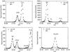 |
Fig. 1 Typical high-resolution mass spectra of ROSINA/DFMS at m/z = 27, 28, 30, and 32, with the well-resolved peaks of HCN and C2H3 at m/z = 27 (top left); CO, N2 and C2H4 at m/z = 28 (top right); NO, CH2O, CH3NH, and C2H6 at m/z = 30 (bottom left); and CH3OH (bottom right). C2H3 is a fragment, while C2H4 may be part parent, part fragment. The background signal (BG) is also shown. |
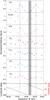 |
Fig. 2 Normalized intensity profiles of various volatiles for September 18, 2014. The error bars represent the ion statistical counting uncertainty, which is calculated as |
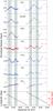 |
Fig. 3 Same as Fig. 2, but for September 29, 2014. Rosetta’s distance from the nucleus of 67P was 18.9 km at a heliocentric distance of 3.23 AU. Where not visible, error bars are smaller than the symbol size. |
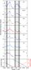 |
Fig. 4 Same as Fig. 2, but for October 11, 2014. Rosetta’s distance from the nucleus was 14.3 km at a heliocentric distance of 3.20 AU. Where not visible, error bars are smaller than the symbol size. |
The cometary signal for each species studied here is well above the spacecraft background (small squares in Fig. 1) that results from spacecraft outgassing (Schläppi et al. 2010). In addition, each of the studied volatile species is clearly resolved by DFMS (e.g., not on the shoulder of another peak; Fig. 1). Background subtraction was performed as in Hässig et al. (2015). Background levels were determined from observations earlier in the mission, when 67P was still relatively far away from the Sun (~3.6 AU), and Rosetta was far from the comet (Aug. 2, 2014; ~900 km). Over time though, cometary material adsorbed onto the spacecraft could add to the background if it is released upon changes in the illumination (slews, etc.), resulting in an additional uncertainty for the absolute signal.
To identify variations on the diurnal timescale, the relative intensity profiles are plotted as a function of time for all analyzed species, along with the sub-spacecraft longitude and latitude in the Cheops coordinate system. The trend of each profile over five rotation periods (Figs. 2 to 4) is then investigated, as well as possible correlations between various species (Figs. 5 and 6). The profiles are normalized to the highest signal to ease the visualization of individual trends. Hence, data are shown in arbitrary units. This study is only concerned with the trend of the intensity profiles and not absolute intensities or absolute densities. Though, the ROSINA/DFMS instrument has been calibrated for a wide range of molecules that were expected at the comet, including the molecules analyzed in this work. Abundances of various species relative to H2O are given in Le Roy et al. (2015).
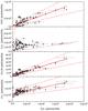 |
Fig. 5 Scatter plots of HCN (top), C2H6 (upper middle), CH3OH (lower middle), and CH4 (bottom) versus H2O. |
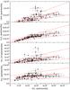 |
Fig. 6 Scatter plots of HCN (top), C2H6 (upper middle), CH3OH (lower middle), and CH4 (bottom) versus CO2. |
3. Results
The intensity profiles of the studied species show various maxima (Figs. 2 to 4). These maxima occur when specific sub-spacecraft longitudes and latitudes are in the view of DFMS. Hence, the term “in view” means the latitude, longitude location of the nadir (sub-spacecraft) direction of the field of view. The sub-spacecraft latitude range in each case below is between −25° and −55°. A summary of the viewing geometry is given in Table 1.
The first identified maximum is characterized by maxima in H2O and all analyzed species. Maxima in all species are seen when the sub-spacecraft longitude is between −100° and −110°, and the well-illuminated neck region is in view. The maxima occur at 13:30 UT on September 18 (Fig. 2), and at 05:40 UT on October 11 (Fig. 4). On September 29, data are missing between ~06:50 UT and 10:30 UT, and between 21:00 UT and 23:15 UT due to reaction wheel offloading; hence, no maxima are observed (Fig. 3). Here we note that the sub-spacecraft longitude and latitude are merely used as guides, as the field of view of ROSINA/DFMS is larger than the size of the nucleus itself. Thus, the longitude and latitude values are given here for reference only, and do not indicate the actual location of outgassing.
Another H2O maximum is observed in the signal at the sub-spacecraft longitude of ~70°, at 20:40 UT on September 18 (Fig. 2); at 02:50 UT and 16:00 UT on September 29 (Fig. 3); and at 13:30 UT on October 11 (Fig. 4). The other polar species CH3OH and HCN also show a maximum, while the apolar species CO2, C2H6, CH4, and CO (which has a relatively small dipole moment) most likely do not. The term most likely is used here because the observed data points at these times and coordinates appear to possibly indicate maxima (see Sep. 18 at 20:40 UT Fig. 2, and Sep. 29 at ~16:00 UT Fig. 3). However, the maximum at 13:30 UT on October 11 indicates that the slightly higher data points at the same longitudes and latitudes seen on September 18 and 29 show the ascending branch leading to maxima at a later time. Thus, it is safe to assume that the CO2, C2H6, CO and CH4 data taken at 20:40 UT and 16:00 UT on September 18 and 29 are also an ascending branch of a later maximum. In this viewing geometry, much of the well-illuminated northern hemisphere is also in the field-of-view, but on the other side of the neck 1/2 rotation away from the first identified H2O maximum.
Maxima independent of the two H2O maxima are also identified in the diurnal intensity profiles. These separate maxima are clear in the cases of CO2, C2H6 and CO, but are missing from the profiles of H2O, HCN, and CH4. CH3OH may or may not also have a small local maximum within the error bars (see CH3OH in Fig. 2 at 17:40 UT, and Fig. 3 at 18:00 UT). The separate maxima are observed in two longitude ranges: once when sub-spacecraft longitudes are between 100° and 140°, as well as between −40° to 10°. The geometry of these longitude ranges corresponds to a view at the poorly illuminated underside of the larger lobe, experiencing winter at the time of the measurements. The separate maxima observed in these fairly narrow longitude and latitude regions occur at 17:40 UT on September 18 (Fig. 2); at 01:30 UT, 05:30 UT, 14:00 UT and 18:00 UT on September 29 (Fig. 3), 2014; and at 02:45 UT and 15:05 UT on October 11 (Fig. 4).
Based on these observations, it is clear that the compositional heterogeneity of the coma of 67P is not limited to the major species H2O, CO2 and CO. In addition, the observed trends of volatiles are not random, but suggest possible correlations. On one hand, the trend of HCN follows that of H2O for all five rotation periods analyzed; on the other hand, CO and C2H6 trend together as well, and follow CO2. It is difficult to tell from the diurnal intensity profiles whether CH3OH follows H2O or CO2 better, while CH4 does not seem to follow either H2O or CO2.
Correlations of minor volatile species with H2O and CO2 are shown in Figs. 5 and 6, respectively. Additional data covering a total of 5 days (~10 rotation periods) were used in the correlation plots. Since this work is concerned with the poorly illuminated southern hemisphere, only data with southern latitude scans were included. Error bars on the points are given by the ion statistical counting uncertainty of the signal  (n is the number of ions detected), and an additional calibration uncertainty of 25%. For the purposes of this study, a linear fit using York-type regression was applied in all cases to confirm the trends observed in the intensity profiles discussed above. While a linear fit may not be the best fit for all cases, it is sufficient to establish or exclude possible correlations by looking for large differences in the fits. In addition, higher-order fits were tested, and do not significantly improve the linear correlations. The dashed lines in Figs. 5 and 6 illustrate the measure of the range in the linear fit (i.e., minimal intercept taken with minimal slope, maximal intercept taken with maximal slope, with an additional 25% uncertainty), taking into account possible systematical errors in the calibration uncertainties. The number of data points that fall outside these lines is given in percentage (Table 2). The signals plotted in Figs. 5 and 6 are not corrected for the detection efficiencies (sensitivities) of the different species, and the resulting slopes do not represent abundances. To avoid being misinterpreted as abundances, the values of the slopes are not given in Table 2. The slopes are positive in every case, with the exception of the C2H6–H2O fit, where the slope is nearly horizontal. A horizontal slope is clearly due to a lack of correlation between these two species.
C2H6 is significantly better correlated with CO2 than with H2O. At the same time, the correlation coefficient is significantly better between HCN and H2O than HCN and CO2. For species that may be difficult to categorize based solely on the time variability of their intensity profiles, such as CH4 and CH3OH, these kinds of correlation plots are especially useful. CH3OH follows H2O in its diurnal variation pattern for the most part (Figs. 3, 4). Though, from a statistical standpoint and considering the large gaps in the CH3OH data sets, a maximum may exist at sub-spacecraft longitudes and latitudes corresponding to the apolar (CO2, C2H6 and CO) maxima that occur independently of H2O maxima (shaded areas in Figs. 2–4). However, when looking at the correlations, CH3OH correlates very well with H2O, while its correlation with CO2 is very poor (Table 2). Hence, CH3OH follows H2O closely. Even if a small local CH3OH maximum were to exist at the locations corresponding to the shaded regions in Figs. 2 to 4, it would not affect its general trend with H2O. The CH4 intensity profile does not appear to follow those of either CO2 or H2O. Indeed, the correlation coefficient of CH4 with CO2 is weak, while a better, but not great, correlation exists between CH4 and H2O (Table 2). Though not shown in Figs. 5 and 6, CO correlates well with CO2 (R2 = 0.79), and poorly with H2O (R2 = 0.30).
Viewing geometry at the discrete maxima identified for the time periods studied.
4. Discussion
The maxima in the intensity profiles of the apolar species (CO, C2H6, and CO2) occur independently of H2O in the southern hemisphere. These apolar species are more volatile than HCN, CH3OH and H2O. Considering that the southern hemisphere was in winter at the time of these measurements while the northern hemisphere was in summer, temperature effects may play a role in the occurrence of the separate maxima in the more volatile species. However, because these maxima occur over a fairly narrow range in longitude in the winter hemisphere rather than over the entire winter hemisphere, the maxima cannot be attributed to temperature differences alone. In an absolute sense, CO2 is more dominant in the southern hemisphere than in the northern hemisphere (Hässig et al. 2015), and so is C2H6 (Le Roy et al. 2015). Higher outgassing of CO2 and C2H6 at lower temperatures is counterintuitive, and implies some sort of heterogeneity superposed on thermal effects. Properties of the ice and/or surface/subsurface (e.g., less and more porous dust coverage, less sintering of the surface) may be different over the longitude-latitude range associated with the independent CO2 (and C2H6, CO, and possibly other species) maxima. Whatever these structural and thermal properties may be, they would favor CO2 sublimation, while inhibiting H2O sublimation, resulting in the higher CO2 and C2H6 densities at these colder, southern hemisphere regions. Therefore, the above results are interpreted to imply heterogeneity within the nucleus.
Fitting parameters for correlation plots.
Nevertheless, heterogeneity within the nucleus may arise from the different parts of the comet receiving different amounts of illumination in each hemisphere over the course of an orbit. Thus, the available heat for conduction to the subsurface could differ significantly between areas in the summer and winter hemispheres. For the time interval studied here, the southern winter hemisphere receives much less illumination than the northern summer hemisphere. Ultimately, differences in illumination lead to differences in the sublimation pattern between certain areas located in the two hemispheres, altering the composition of the surface and subsurface. The fact that polar and apolar volatile species demonstrate a different sublimation pattern may be indicative of at least two phases of ice in 67P. The apolar ice phase composed of CO2, C2H6, and also CO (but not CH4; see later in the text) would be segregated from the polar ice phase (H2O, CH3OH, HCN) over this southern-hemisphere narrow longitude-latitude region to result in the observed sublimation behavior in correlation with the rotational phase of the nucleus. If such an apolar ice phase were exposed in response to a previous intense southern-hemisphere summer, it would be releasing material of differing composition than the ice in other areas of the nucleus. Structural and thermal properties still need to be different from other parts of the nucleus over this narrow longitude-latitude southern hemisphere region. These properties only enable exposure of more volatile ices in this region, rather than all across the southern hemisphere. Temperatures over the southern hemisphere would still be too cold to sublimate the less volatile, polar species (H2O, CH3OH, HCN) at the time of these observations. Therefore, the lack of maxima in H2O, CH3OH and HCN over this longitude region in the southern hemisphere does not necessarily imply that these species are not present in the southern hemisphere. Instead, CO2 and more volatile species sublimate while H2O and other less volatile species do not, which suggests an upper temperature limit somewhere between 80–140 K (bracketing the sublimation temperatures of CO2 and H2O, respectively, as determined from Fray & Schmitt 2009 for a pressure of 10-11 bar) in the sublimating subsurface layer over the longitude-latitude range in question.
The H2O, CH3OH and HCN maxima observed without corresponding maxima in CO2, C2H6 and CO (at longitude 70°; see Table 1) are also strongly indicative of thermal evolutionary heterogeneity. This viewing geometry allows a larger portion of the well-illuminated summer hemisphere to be in the field-of-view of ROSINA/DFMS, which adds H2O, CH3OH and HCN to the detected signal. This location is depleted in the more volatile species though, most likely as a result of sublimation, while the less volatile species are still present and sublimate. Based on the similar behavior of Hartley 2 in terms of H2O dominated outgassing from the neck/waist as opposed to CO2 dominant outgassing from one of the lobes, a similar redeposition of icy grains to the neck/waist region could be envisaged for 67P. However, the overall activity of Hartley 2 was significantly higher than the activity of 67P at the time of observation. The EPOXI measurements of Hartley 2 were obtained shortly after its perihelion, while 67P was significantly farther (~3 AU) from the Sun at the times of the ROSINA/DFMS measurements reported here. The CO2 outgassing, which was found to drive the overall activity of Hartley 2, is much lower farther away from the Sun; hence, the number of H2O ice clumps that would be dragged along is expected to be less significant as well. The diverse spatial distribution of volatiles was interpreted as separate polar and apolar ice phases in the case of Hartley 2 (Mumma et al. 2011). If redeposition of H2O ice clumps (with other polar species) is in fact occurring on 67P, and is responsible for the observed maxima in the peak count rates, such a layer would be sublimating directly from the surface. The sublimation characteristics of a redeposited layer would then be different from the characteristics of other areas in the northern hemisphere (e.g., the neck, where all species show maxima), in agreement with what is observed. The redeposited ice, if present, should be observed directly on the surface by other Rosetta instruments. Perhaps the large compositional difference seen by OSIRIS in the Hapi region relative to other regions (Sierks et al. 2015) characterized by a low (bluer) spectral slope (Fornasier et al. 2015) may be indicative of such redeposition of H2O ice.
The above discussion is supported by the correlations shown in Figs. 5, 6, and Table 2. HCN and CH3OH are clearly well correlated with H2O, while C2H6 correlates well with CO2 in the southern, winter hemisphere. When correlation between two species exists, the intercept carries physical meaning. An intercept passing through the origin indicates that the two molecules are released together. The intercept of the linear fit to HCN and H2O passes through zero within the uncertainties (see dashed lines in Fig. 5, top), implying that the two molecules are released together, and HCN follows H2O. This combined release implies that if the HCN detected by ROSINA/DFMS may be emanating from HCN polymers in dust, then the polymers must come off together with H2O. A combined release would be the case if these polymers (and dust) covered H2O ice on the surface, and/or if the dust grains were lifted off the surface. Statistically, the intercept passes through zero for the correlation of CH3OH with H2O as well. This co-release of HCN and CH3OH with H2O supports the possible presence of a polar ice phase, as discussed earlier. The same is true for C2H6 and CO2, which are also released from the nucleus together. Though, the signal is corrected for spacecraft background that might be slightly overestimated, as mentioned in Sect. 2. Subtraction of an overestimated background would affect where the intercept passes through the axes. If too high a spacecraft background is assumed for the species on the y-axis, then too much is subtracted from the signal, and the intercept passes through at a lower value than it would with the true background. The same applies for species on the x-axis. Therefore, it should be noted that the above interpretations assume that only signal due to spacecraft outgassing was subtracted in the background correction.
Although apolar, CH4 shows an irregular diurnal trend. Surprisingly, CH4 is uncorrelated with CO2, and is slightly, but still poorly correlated with H2O. This behavior is difficult to explain by thermal effects, where CH4 is expected to sublimate with, or even before the apolar CO2, suggesting that CH4 should follow CO2. On the other hand, if CH4 was mixed in the H2O ice matrix, it should sublimate together with H2O, and should follow the trend of H2O better than what is observed here. On the contrary, CH4 displays a distinct behavior from both polar and apolar species. This behavior is not due to low signal-to-noise ratio for CH4, as the cometary signal for CH4 is well above background. Similarly to CO2 and C2H6, CH4 is also more abundant in an absolute sense in the southern hemisphere in winter at the time of these observations than in the northern hemisphere (Le Roy et al. 2015). In fact, CH4 does not follow CO closely either based on Figs. 2–4, which is also unexpected considering their similarly low equilibrium sublimation temperatures. The R2 value between CH4 and CO is 0.43. The unique CH4 trend is intriguing, and suggests that additional mechanisms and/or properties of the nucleus need to be considered to fully understand these observations. For instance, CH4 has been demonstrated to readily form clathrate hydrates under nebular conditions (e.g., Lunine & Stevenson 1985; Mousis et al. 2010). Though, CH4 not following H2O closely, and the intercept of the linear fit not passing through the origin (Fig. 5, bottom panel) shows that the presence of CH4 clathrates cannot exclusively explain the behavior observed by ROSINA/DFMS either.
5. Conclusions
Analysis of various volatile species measured in the coma by ROSINA/DFMS showed that the coma heterogeneity identified in Hässig et al. (2015) is not limited to H2O, CO2 and CO. C2H6, HCN, CH3OH, and CH4 also show heterogeneity in the coma. The intensity profiles of the analyzed volatiles either follow H2O or CO2 more closely. The observed heterogeneity in the coma of 67P suggests heterogeneity in the southern hemisphere of the nucleus. In addition, the correlation among volatile species and H2O and CO2 may also indicate that two distinct phases of ice dominated by polar versus apolar species exist in the nucleus of 67P.
The obliquity of the spin axis of 67P results in drastic differences between the length and intensity of seasons in the two hemispheres. Perihelion occurs when the southern hemisphere is in summer, resulting in shorter but hotter summers than in the northern hemisphere. In response to the hemispheric differences in insolation, the southern hemisphere nucleus could have been stripped of layers several meters deep over the short, intense southern summers. This process could expose larger amounts of highly volatile species still present at greater depths in the nucleus. These exposed areas could then sublimate farther away from the Sun, while it is still too cold for H2O and the other polar species to sublimate. However, the irregular behavior of CH4 suggests that this picture is likely more complicated, with additional processes and/or nucleus properties superposed on thermal evolutionary effects. While primordial heterogeneity could also explain the observed coma profiles of the studied volatiles, such implication is premature, and can only be taken as tentative at this point.
The diurnal intensity profiles of the studied volatiles in the coma are expected to change as the seasons on 67P change, and the southern hemisphere gradually warms up. These changes will be crucial to understanding the source of heterogeneity. If maxima appear in the less volatile species in the southern hemisphere, then temperature is an important driver of the features reported here, and phases of polar and apolar ices may exist in segregation. Any lack of H2O, CH3OH, and HCN maxima appearing in the southern hemisphere as the seasons change may be an indicator of primordial heterogeneity. Possible changes in CH4, or the lack thereof, will be crucial in the accurate interpretation of the data. These predictions for the expected changes in the diurnal coma profiles will be useful when the southern hemisphere begins to warm up in May 2015.
Future analysis of additional volatile constituents (such as sulfur compounds) is warranted in the context of this work. The reasons behind the observed irregular release of CH4 from the nucleus of 67P will be further investigated, and its possible correlation with H2O and CO will be tested with later observations at smaller heliocentric distances. In addition, the question of polar versus apolar outgassing will continue to be explored based on future observations. Simultaneously, development of a detailed heterogeneous nucleus model is crucial for the accurate interpretation of these measurements. The physics of such a heterogeneous model need to be placed in context with well-developed evolutionary, compositional, and structural models of cometary nuclei.
Acknowledgments
The authors acknowledge support from the following institutions and agencies: work at the Southwest Research Institute was supported by subcontract No. 1496541 from the Jet Propulsion Laboratory (JPL). The work at the University of Bern was funded by the State of Bern, the Swiss National Science Foundation, and the European Space Agency PRODEX Program. This work has been carried out thanks to the support of the A*MIDEX project (No. ANR-11-IDEX-0001-02) funded by the “Investissements d’Avenir” French Government program, managed by the French National Research Agency (ANR). This work was supported by CNES grants at LATMOS; LPC2E. Work at BIRA-IASB was supported by the Belgian Science Policy Office via PRODEX/ROSINA PEA 90020. Work at the University of Michigan was funded by NASA under contract JPL-1266313. These results from ROSINA would not be possible without the work of the many engineers, technicians, and scientists involved in the mission, in the Rosetta spacecraft, and in the ROSINA instrument team over the past 20 years, whose contributions are gratefully acknowledged. We thank herewith the work of the whole European Space Agency (ESA) Rosetta team. Rosetta is an ESA mission with contributions from its member states and NASA. All ROSINA data are available on request until they are released to the Planetary Science Archive of ESA and the Planetary Data System archive of NASA. The authors would also like to thank Michael DiSanti for his valuable feedback, which helped improve this paper.
References
- A’Hearn, M. F. 2011, ARA&A, 49, 281 [NASA ADS] [CrossRef] [Google Scholar]
- A’Hearn, M. F., Belton, M. J. S., Delamere, W. A., et al. 2011, Science, 332, 1396 [NASA ADS] [CrossRef] [Google Scholar]
- A’Hearn, M. F., Feaga, L. M., Keller, H. U., et al. 2012, ApJ, 758, 29 [NASA ADS] [CrossRef] [Google Scholar]
- Balsiger, H., Altwegg, K., Bochsler, P., et al. 2007, Space Sci. Rev., 128, 745 [NASA ADS] [CrossRef] [Google Scholar]
- Belton, M. J. S., Thomas, P., Veverka, J., et al. 2007, Icarus, 187, 332 [NASA ADS] [CrossRef] [MathSciNet] [Google Scholar]
- Bieler, A., Altwegg, K., Balsiger, H., et al. 2015, A&A, 583, A7 [NASA ADS] [CrossRef] [EDP Sciences] [Google Scholar]
- Bockelée-Morvan, D., Crovisier, J., Mumma, M. J., & Weaver, H. A. 2004, in The composition of cometary volatiles, ed. G. W. Kronk, 391 [Google Scholar]
- Bonev, B. P., Mumma, M. J., Radeva, Y. L., et al. 2008, ApJ, 680, L61 [NASA ADS] [CrossRef] [Google Scholar]
- Feaga, L. M., A’Hearn, M. F., Sunshine, J. M., Groussin, O., & Farnham, T. L. 2007, Icarus, 190, 345 [NASA ADS] [CrossRef] [Google Scholar]
- Fornasier, S., Hasselmann, P. H., Barucci, M. A., et al. 2015, A&A, 583, A30 [NASA ADS] [CrossRef] [EDP Sciences] [Google Scholar]
- Fray, N., & Schmitt, B. 2009, Planet. Space Sci., 57, 2053 [NASA ADS] [CrossRef] [Google Scholar]
- Hässig, M., Altwegg, K., Balsiger, H., et al. 2013, Planet. Space Sci., 84, 148 [NASA ADS] [CrossRef] [Google Scholar]
- Hässig, M., Altwegg, K., Balsiger, H., et al. 2015, Science, 347, 276 [CrossRef] [Google Scholar]
- Jorda, L., Gaskell, R., Hviid, S. F., et al. 2015, Shape models of 67P/Churyumov-Gerasimenko, RO-C-OSINAC/OSIWAC-5-67P-SHAPE-V1.0., NASA Planetary Data System and ESA Planetary Science Archive [Google Scholar]
- Le Roy, L., Altwegg, K., Balsiger, H., et al. 2015, A&A, 583, A1 [Google Scholar]
- Lunine, J. I., & Stevenson, D. J. 1985, ApJS, 58, 493 [NASA ADS] [CrossRef] [Google Scholar]
- Mottola, S., Lowry, S., Snodgrass, C., et al. 2014, A&A, 569, L2 [NASA ADS] [CrossRef] [EDP Sciences] [Google Scholar]
- Mousis, O., Lunine, J. I., Picaud, S., & Cordier, D. 2010, Faraday Discussions, 147, 509 [NASA ADS] [CrossRef] [Google Scholar]
- Mumma, M. J., Bonev, B. P., Villanueva, G. L., et al. 2011, ApJ, 734, L7 [NASA ADS] [CrossRef] [Google Scholar]
- Rickman, H., Marchi, S., A’Hearn, M. F., et al. 2015, A&A, 583, A44 [NASA ADS] [CrossRef] [EDP Sciences] [Google Scholar]
- Rubin, M., Altwegg, K., Balsiger, H., et al. 2015, Science, accepted [Google Scholar]
- Schläppi, B., Altwegg, K., Balsiger, H., et al. 2010, J. Geophys. Res. (Space Phys.), 115, 12313 [Google Scholar]
- Sierks, H., Barbieri, C., Lamy, P. L., et al. 2015, Science, 347, 1044 [NASA ADS] [CrossRef] [Google Scholar]
All Tables
All Figures
|
Fig. 1 Typical high-resolution mass spectra of ROSINA/DFMS at m/z = 27, 28, 30, and 32, with the well-resolved peaks of HCN and C2H3 at m/z = 27 (top left); CO, N2 and C2H4 at m/z = 28 (top right); NO, CH2O, CH3NH, and C2H6 at m/z = 30 (bottom left); and CH3OH (bottom right). C2H3 is a fragment, while C2H4 may be part parent, part fragment. The background signal (BG) is also shown. |
| In the text | |
|
Fig. 2 Normalized intensity profiles of various volatiles for September 18, 2014. The error bars represent the ion statistical counting uncertainty, which is calculated as |
| In the text | |
|
Fig. 3 Same as Fig. 2, but for September 29, 2014. Rosetta’s distance from the nucleus of 67P was 18.9 km at a heliocentric distance of 3.23 AU. Where not visible, error bars are smaller than the symbol size. |
| In the text | |
|
Fig. 4 Same as Fig. 2, but for October 11, 2014. Rosetta’s distance from the nucleus was 14.3 km at a heliocentric distance of 3.20 AU. Where not visible, error bars are smaller than the symbol size. |
| In the text | |
|
Fig. 5 Scatter plots of HCN (top), C2H6 (upper middle), CH3OH (lower middle), and CH4 (bottom) versus H2O. |
| In the text | |
|
Fig. 6 Scatter plots of HCN (top), C2H6 (upper middle), CH3OH (lower middle), and CH4 (bottom) versus CO2. |
| In the text | |
Current usage metrics show cumulative count of Article Views (full-text article views including HTML views, PDF and ePub downloads, according to the available data) and Abstracts Views on Vision4Press platform.
Data correspond to usage on the plateform after 2015. The current usage metrics is available 48-96 hours after online publication and is updated daily on week days.
Initial download of the metrics may take a while.