| Issue |
A&A
Volume 583, November 2015
|
|
|---|---|---|
| Article Number | A92 | |
| Number of page(s) | 12 | |
| Section | Cosmology (including clusters of galaxies) | |
| DOI | https://doi.org/10.1051/0004-6361/201526001 | |
| Published online | 02 November 2015 | |
Polarized cosmic microwave background map recovery with sparse component separation
Laboratoire CosmoStat, AIM, UMR CEA-CNRS-Paris 7, Irfu, SAp/SEDI, Service
d’Astrophysique, CEA Saclay,
91191
Gif-sur-Yvette Cedex,
France
e-mail:
This email address is being protected from spambots. You need JavaScript enabled to view it.
Received: 2 March 2015
Accepted: 29 July 2015
Abstract
The polarization modes of the cosmological microwave background are an invaluable source of information for cosmology and a unique window to probe the energy scale of inflation. Extracting this information from microwave surveys requires distinguishing between foreground emissions and the cosmological signal, which means solving a component separation problem. Component separation techniques have been widely studied for the recovery of cosmic microwave background (CMB) temperature anisotropies, but very rarely for the polarization modes. In this case, most component separation techniques make use of second-order statistics to distinguish between the various components. More recent methods, which instead emphasize the sparsity of the components in the wavelet domain, have been shown to provide low-foreground, full-sky estimates of the CMB temperature anisotropies. Building on sparsity, we here introduce a new component separation technique dubbed the polarized generalized morphological component analysis (PolGMCA), which refines previous work to specifically work on the estimation of the polarized CMB maps: i) it benefits from a recently introduced sparsity-based mechanism to cope with partially correlated components; ii) it builds upon estimator aggregation techniques to further yield a better noise contamination/non-Gaussian foreground residual trade-off. The PolGMCA algorithm is evaluated on simulations of full-sky polarized microwave sky simulations using the Planck Sky Model (PSM). The simulations show that the proposed method achieves a precise recovery of the CMB map in polarization with low-noise and foreground contamination residuals. It provides improvements over standard methods, especially on the Galactic center, where estimating the CMB is challenging.
Key words: methods: data analysis / cosmic background radiation / methods: statistical
© ESO, 2015
1. Introduction
The cosmic microwave background (CMB) provides a snapshot of the state of the Universe at the time of recombination. It therefore carries invaluable information about the infancy of the Universe and its evolution to the current state. After a series of full-sky measurements of the microwave sky (COBE, Bennett et al. 1996; WMAP, Bennett 2013), Planck (Planck Collaboration XII 2014) has recently released an accurate estimate of the CMB temperature map. Studying the statistical properties of the CMB temperature maps already provides a huge amount of information about the primordial state of the Universe. Additionally, the CMB map is a radiation with linear polarization that is described by the three polarization modes T,E, and B (Hu & White 1997); these three modes are observed through the Stokes parameters T,Q, and U. The information carried by CMB polarization is crucial for i) improving the estimation of the cosmological parameters and breaking some of their degeneracies; and it ii) provides privileged access to probe the energy scale of inflation through estimating the scalar-to-tensor ratio r and the tensor spectral index nt. Indeed, inflationary models predict the presence of tensor perturbations, which would be traced by the presence of specific CMB B-modes.
From the first full-sky observations of CMB temperature anisotropies by the Cosmic Background Explorer (COBE – see Bennett et al. 1996) to the Planck 2013 results (Planck Collaboration XII 2014), much attention has been paid to the estimation of temperature anisotropies by component separation and little to the polarization signal. In contrast to temperature, polarization anisotropies are more challenging to measure as their level is about five orders of magnitude lower than the temperature anisotropy level.
Polarization anisotropies have first been measured by balloon (Masi et al. 2006) and ground-based experiments such as Cosmic Background Imager (CBI; Readhead 2004). The Wilkinson Microwave Anisotropy Probe (WMAP) experiments more recently provided full-sky observations of the polarization anisotropies (Bennett 2013). The BICEP2 (Background Imaging of Cosmic Extragalactic Polarization) collaboration initially announced the detection of inflationary B-modes and a measurement of the scale-to-tensor ratio r = 0.2, which would be slightly different from the Planck 2013 and 2015 results (Planck Collaboration XIII 2015), which derived a stronger constraint r< 0.11 (95% confidence interval). If this discrepancy could have found various cosmological explanations, a polarized foregrounds origin was soon advocated (see Flauger et al. 2014; Mortonson & Seljak 2014). This point was later supported by a study of dust polarization made available by the Planck consortium (Planck Collaboration Int. XXXII 2014) and joint BICEP2/Planck investigations (BICEP2/Keck 2015). This controversy highlights the central role played by foreground cleaning and component separation to provide an accurate estimation of polarized CMB maps.
Component separation methods have lately mainly focused on temperature analysis (Leach et al. 2008; Basak & Delabrouille 2012b; Bobin et al. 2013a,b, 2014b). Most component separation techniques rely on a linear mixture model. According to this model, each observation of the sky xi at wavelength νi is modeled as the linear combination of n components { sj } j = 1,...,n:  (1)where aij stands for the contribution of component sj in observation xi and ni models instrumental noise. In this model, the data are assumed to be at the same resolution. This model can be more conveniently recast in matrix form:
  (2)where each observation xi is stored in the ith row of the observation matrix X, S is the source matrix, A is the mixing matrix, and N models instrumental noise. From a physical point of view, the jth column of A, which we denote by aj, contains the electromagnetic spectrum of the source sj.
Better known as blind source separation (BSS) in statistics and signal processing (Comon & Jutten 2010), component separation aims at estimating the mixing matrix A and the sources S from the knowledge of the observations X. This is a classical ill-posed inverse problem, which admits an infinite number of solutions. Distinguishing physically relevant components from erroneous estimates furthermore requires imposing some desired properties on the components to be retrieved. In the framework of BSS, component separation methods generally enforce some diversity or contrast to distinguish between distinct components. To the best of our knowledge, all standard component separation methods for polarized CMB observations build upon second-order statistics (Eriksen et al. 2004; Bennett 2013; Kim et al. 2009; Aumont & Macías-Pérez 2007).
Lately, building on different grounds, a novel component separation technique, the local-generalized morphological component analysis (LGMCA), see Bobin et al. (2013a), has been introduced. In contrast to standard component separation techniques, the LGMCA algorithm relies on the sparse representation of Galactic foregrounds, which makes it more sensitive to the higher-order statistics of these components. Using GMCA, a joint WMAP-Planck high-quality full-sky CMB map has been reconstructed. Additionally, this map has been shown to be free of detectable thermal Sunyaev-Zel’Dovich (SZ) emission (Sunyaev & Zeldovich 1970) and to have only low foreground contamination (Bobin et al. 2014b). The resulting CMB temperature map has been used to analyze the large-scale anomalies of the CMB radiation. Thanks to its low level of foregrounds, masking of the Galactic center was not necessary for CMB large-scale studies (Rassat et al. 2014; Ben-David & Kovetz 2014; Aiola et al. 2015; Lanusse et al. 2014).
Contributions
Building upon the concept of sparse signal representation, we here introduce an extension of the LGMCA algorithm to compute an accurate estimate of the CMB polarized maps with animproved noise/non-Gaussian foreground contamination trade-off. In contrast to the processing of CMB temperature data, estimating the CMB polarization anisotropies is an even more challenging task since the polarization signal is weak and dominated by Galactic foregrounds and noise contamination. For that purpose, the proposed method, dubbed polarized GMCA (PolGMCA), builds upon two new key mechanisms: i) it profits from recent advances in BSS that allow for the efficient separation of sparse and partially correlated sources; and ii) it builds upon map estimator aggregation, which helps providing a better balance between foreground residuals and noise contamination. The PolGMCA algorithm is detailed in Sect. 2. Numerical experiments based on the Planck Sky Model are described in Sect. 3, which demonstrate the ability of the proposed method to achieve good separation performances on the Galactic center as well as at large scales.
2. Polarized sparse component separation
2.1. Component separation for polarized data
Modeling of polarized data:
polarized fields can be described in several ways. They are generally measured by the Stokes parameters Q and U, which can further be expanded in the harmonic domain as follows:  (3)where
  stands for the spin-2 spherical harmonics basis functions.
Extending the concept of the wavelet representation for polarization vector fields on the sphere has been proposed in Starck et al. (2009) based on the celebrated “a trous” algorithm (Starck et al. 2006). Building a wavelet transform for Q/U polarization fields then consist of building J successive smooth approximations of the Q and U maps via a convolution with dyadically rescaled versions of the so-called scaling function h:  where J stands for the total number of scales. Following Starck et al. (2006), the scaling function is built so as to verify isotropy in the pixel domain. The wavelet coefficients at scale j are then defined as the difference of two consecutive approximations:
  In practice, these operations reduce to simple multiplications of the Q and U map spherical harmonics coefficients with the scaling filters { hj } j = 0,...,J.
According to the à trous algorithm, the Q and U maps can be reconstructed by a very simple summation:  The same polarization field can equivalently be described as E and B polarization modes (Zaldarriaga 1998):
  where Yℓm stands for the standard 0-spin spherical harmonics functions. The E and B fields are therefore usual real scalar fields. The expansions of the E and B fields in the harmonics domain is related to the Q and U fields as follows:
  The E and B fields are therefore derived from the Q and U fields by simply applying twice the spin-lowering operator to Q + iU and the spin-raising operator to Q − iU. Following (Starck et al. 2009), extending the isotropic and undecimated wavelet transform for E/B polarization fields by constructing formal E and B maps as described in Eq. (10) from the Q and U maps and then applying the isotropic undecimated wavelet transform for each E and B scalar-valued maps independently.
Standard approaches for polarized CMB map estimation:
component separation on a polarization vector field can be performed either in the Q/U coordinate system or the E/B field. So far, most standard methods use a description of the components based on second-order statistics. In that respect, the CMB is more naturally described by its E/B power spectra and cross-spectra in the E and B fields. Therefore, the following advanced methods perform in the E/B fields:
-
Internal linear combination – ILC: this component separation technique is well known in the astrophysics community (Eriksen et al. 2004; Bennett 2013; Kim et al. 2009). Essentially, it estimates a CMB map, whether in temperature or polarization, with minimum variance. The Needlet-ILC (Basak & Delabrouille 2012a) performs in the wavelet domain; it has been applied to the WMAP data and more recently to the Planck PR2 data (Planck Collaboration IX 2015) to provide estimates of the CMB polarized maps. In statistics, this estimation procedure is well known as the best linear unbiased estimator, or BLUE.
-
Spectral matching ICA – SMICA: this component separation method enforces the statistical independence of the sought-after components – for more details, see (Cardoso et al. 2002; Delabrouille et al. 2003). SMICA assumes that each component, whether the CMB or foreground components, can be modeled as a random Gaussian random field with unknown power spectrum. In this setting, the components are estimated by enforcing the contrast between the spectrum of the components in the harmonic domain. An extension of SMICA to polarized data has been proposed in Aumont & Macías-Pérez (2007).
The main limitations of these two component separation techniques are twofold: i) galactic and extragalactic foregrounds can hardly be modeled as stationary and homogeneous signals; and ii) they both rely on second-order statistics to separate the components, which is not well-suited to model Galactic foregrounds: they are non-stationary and non-Gaussian signals in nature.
More recently, based on the concept of sparsity, we introduced a new component separation technique called GMCA (Bobin et al. 2013a). This algorithm is based on the sparse modeling of the foregrounds in the wavelet domain. In contrast to the CMB field, the Galactic foregrounds are better described in the data domain, and therefore in the Q and U maps. We therefore prefer using the GMCA algorithm on the observed Q and U maps.
In early 2015, the Planck consortium released the first estimates of the polarized CMB maps that have been computed from the Planck PR2 observations (Planck Collaboration IX 2015). The proposed four maps have been calculated using extensions to polarization of the component separation methods used to process CMB temperature maps Planck Collaboration XII (2014). These methods include the following:
-
Commander (Eriksen et al. 2008): this is a Bayesian parametric estimation method that relies on an explicit parameterized modeling of the sky, which includes CMB, synchrotron, and thermal dust emissions.
-
SEVEM(Fernández-Cobos et al. 2012): this is a template-fitting method that performs in the wavelet domain. For this purpose, templates are derived from differences of input Planck observations and are used as templates in a foreground-cleaning procedure.
-
NILC:a version of the Needlet ILC algorithm has been used to derived polarized CMB maps. More precisely, the NILC estimates ILC weights in 13 wavelet bands (see Planck Collaboration IX 2015).
-
SMICA:a special version of the SMICA algorithm (Cardoso et al. 2002; Delabrouille et al. 2003) has been used to process the Planck PR2 data. In contrast to the original SMICA algorithm, spectral parameters are fitted for ℓ ≤ 50. For larger multipoles, it is a harmonic ILC.
Component separation precisely amounts to estimating a mixing matrix A, as described in Eq. (2), or equivalently unmixing coefficients for ILC-based methods. As in Aumont & Macías-Pérez (2007), Basak & Delabrouille (2012a), these parameters can be estimated jointly for both the E and B fields, which makes perfect sense for the CMB, but not necessarily for foreground emissions. Indeed, allowing for different mixing matrices for the Q/U or E/B allows for more degrees of freedom to distinguish between complex contaminants, which are not perfectly described by the linear mixture model of 2. Below, we propose performing the GMCA algorithm independently in the Q and U fields.
2.2. Sparse component separation with GMCA
In contrast to standard component separation methods in cosmology, GMCA (Bobin et al. 2013a) relies on a different separation principle: it profits from the naturally sparse distribution of astrophysical components in the wavelet domain. More precisely, the so-called sparsity property means that most of the energy content of the components is concentrated in a few coefficients. This property is also shared by the CMB since its power spectrum decays rapidly (i.e., ℓ2 at large scale and ℓ3 at small scales). This entails that the energy of the CMB will be mainly concentrated in a small number of wavelet coefficients. Components of distinct physical origins are very likely to exhibit different sparsity patterns. The GMCA algorithm assumes that the components are unlikely to share similar high-amplitude wavelet coefficients. Enforcing the sparsity of components in the wavelet domain has indeed been shown to be an efficient separation procedure to achieve a clean, low-foreground estimate of the CMB temperature anisotropies (Bobin et al. 2013a, 2014b).
Let Φ denotes a wavelet transform. We assume that each source si can be sparsely represented in Φ; sj = αjΦ. The data X can be written as  (14)where α is an Ns × T matrix whose rows are αj. The GMCA algorithm estimates a mixing matrix A that leads to the sparsest sources S. In practice, this is achieved by solving the following optimization problem
 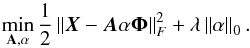 (15)The expression ∥α∥0 stands for ℓ0 pseudo-norm of α, which counts the number of non-zero entries of α. The term
  stands for the Frobenius norm.
The problem in Eq. (15) is solved by using an iterative algorithm that optimizes sequentially on the sources S = αΦ and the mixing matrix A. According to the model in Eq. (2), the GMCA algorithm needs to be applied on data that share the same resolution. For that purpose, the Planck frequency channels are first downgraded to a common resolution before applying GMCA; a high-resolution CMB map estimate is then carried out by performing GMCA on various subsets of the Planck data. We refer to Bobin et al. (2013a) for more details about the GMCA algorithm.
Accounting for the variability of the mixture model: in polarization as well as in temperature, most foreground emissions, such as the thermal dust and synchrotron emissions, have an electromagnetic spectrum that varies across the sky. From a mathematical point of view, this causes the mixing matrix A to vary across pixels. To account for the heterogeneity of the mixture, the GMCA algorithm is applied on sky patches in each wavelet band. These different steps gave birth to the local-GMCA (LGMCA) algorithm, which has been described in detail in Bobin et al. (2013a).
The LGMCA algorithm has been implemented and evaluated on simulated Planck data in Bobin et al. (2013a). It has been applied to the Planck PR1 data, for which it led to the estimation of a low-foreground full-sky map of the CMB anisotropies Bobin et al. (2014b).
2.3. Sparse reconstruction of the CMB polarization maps
Separating non-Gaussian and partially correlated components.
Whether in polarization or in temperature, foreground removal is an extremely challenging task, particularly in two respects.
-
In the Galactic center: the foregrounds in Galactic regions are by far the contaminants with the largest emissivity. The rapid variation of the foreground emission laws in the vicinity of the Galactic center makes component separation strenuous, in particular for synchrotron and thermal dust emissions. This has been addressed in Bobin et al. (2013a) by localizing the mixture model in the framework of GMCA. However, distinct components are also prone to share some similarities in the Galactic region: different components have high emissivity in the same regions. Subsequently, distinct components will exhibit partial correlations in these areas. This phenomenon makes separating them much more difficult.
-
At large scales: in this case – typically for ℓ< 100 – only few spherical harmonics are observed. As a consequence, even theoretically decorrelated components exhibit some experimental correlation, commonly dubbed chance-correlations. The underlying components can therefore be regarded as partially correlated signals.
In both cases, the presence of partial correlations between the components will strongly hamper the performances of component separation methods and weaken their ability to efficiently remove Galactic foregrounds from the cosmological signal. An extension of the GMCA algorithm (Bobin et al. 2014a) has recently been introduced in the signal-processing community to specifically solve the separation of partially correlated sources. Its main assumption is that partial correlation between components will mainly impact a subset of the sparse decomposition coefficients. The rationale of this algorithm relies on a weighting scheme that aims at penalizing correlated entries, which are the most detrimental for separation. This algorithm first means that some diagonal weight matrix Q (Bobin et al. 2014a) needs to be defined, and secondly that the minimization problem in Eq. (15) needs to be substituted by 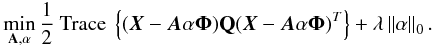 (16)Bobin et al. (2014a) have shown that partially correlated samples are related to non-sparse columns of the source matrix S. Based on this relationship, it adaptively updates the weight matrix with respect to the estimated sources during the iterations of the algorithm.
This algorithm has been shown to be very effective in distinguishing partially correlated sources. For more details, we refer to Bobin et al. (2014a).
Improving the noise/foreground residual trade-off by combining estimators.
Whether in temperature or in polarization, an accurate estimate of CMB anisotropies requires solving somewhat antagonistic signal-processing problems:
-
Low noise contamination: polarized CMB data are highly dominated by instrumental noise, by several orders of magnitude. An effective CMB recovery method should therefore be able to deliver polarized CMB map estimates with low noise contamination. Instrumental noise in Planck-like data is generally approximated by a stationary Gaussian random field. Hence methods based on second-order statistics (SOS) in the harmonic domain, such as harmonic ILC (HILC, Kim et al. 2009), are very efficient at small scales where noise dominates.
-
Low foreground residuals: foregrounds, and especially Galactic foregrounds, are non-Gaussian and non-stationary signals. As a consequence, component separation methods that rely on SOS, and particularly in the harmonic domain, are poorly suited to accurately remove foreground components. Bobin et al. (2013a) emphasized that the use of sparsity in spatially localized signal representations, such as wavelets, provides an effective strategy to estimate a low-foreground CMB map.
These two points underline that component separation for CMB polarization data differs from the case of temperature where the noise is not as high as at the level of foreground components. Neither SOS-based nor sparsity-based techniques are perfect candidates to estimate low-foreground and low-noise CMB polarization maps. Subsequently, we instead propose to combine estimates delivered by SOS-based and sparsity-based component separation methods. This aggregation of complementary estimators is inspired by advances in statistics and estimation theory (Yang 2004).
For the sake of generality, we assume that we have access to P unbiased estimators of the CMB { ci } i = 1,...,P, which basically differ from each other by their noise contamination and level of foreground residuals. The goal of estimator aggregation is to find some weights { πi } i = 1,...,P so that the combined estimator is expressed as a linear combination of these estimators:  (17)The resulting estimator is guaranteed to be unbiased as long as the weights add up to unity:
  . Furthermore, the weights are estimated by minimizing some cost function ℛ(π1,...,πP):
 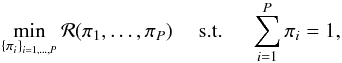 (18)which enforces some desired properties for the combined estimator.
Essentially, the proposed estimator aggregation procedure will amount to combining SOS-based CMB map estimates, delivered by the HILC, with sparsity-based estimates provided by the LGMCA algorithm. The LGMCA algorithm is well-suited for accurately removing foreground residuals, but does not provide a low-noise estimate. In that respect, estimator combination is mainly implemented so as to minimize the impact of instrumental noise. Since noise is best modeled in the harmonic domain with second-order statistics, it is therefore natural to combine LGMCA-based estimates with HILC by seeking the weights { πi } i = 1,...,P that minimize the variance of the estimated CMB in the harmonic domain.
In practice, a combined estimator in the harmonic domain is derived by decomposing the harmonic domain in overlapping bins of multipoles of fixed width Δ, which are indexed by l. A set of weights { πi,l } i = 1,...,P is then estimated in each band of multipoles. Consequently, the aggregation of the P estimators { ci } i = 1,...,P is carried out by solving the following minimization problem in each band l of multipoles: 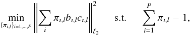 (19)where ∥ . ∥ ℓ2 denotes the Euclidean norm, the term ci,l stands for the lth harmonic multipole of the ith CMB map, and the values bi,l are the beam of different maps at the lth harmonic multipole. This estimator is better known as the best linear unbiased estimator (BLUE) in the statistics community or the ILC in astrophysics. The different weights are then recombined to provide values for each multipole ℓ.
Interestingly, the LGMCA algorithm amounts to applying the GMCA algorithm on various subsets of observations. This yields various estimates of the CMB maps with various spatial resolutions: estimated maps with the lowest resolution are computed from a larger number of observations and vice versa. We have pointed out in Bobin et al. (2014b) that applying component separation to a large number of observations allows for more degrees of freedom to better provide a clean estimate of the CMB map. The current version of the LGMCA algorithm performs by using a single CMB map estimate in each wavelet band. From the perspective of estimator aggregation, the LGMCA algorithm already combines complementary CMB maps, but in a rather suboptimal way. Again, the framework of estimator aggregation can help providing a more efficient combination of GMCA-based estimators with a better balance between noise contamination (i.e., using maps with different spatial resolutions) and foreground residual (i.e., using maps obtained from various subsets of data).
The PolGMCA algorithm therefore i) derives five estimates of the CMB map from various subsets of observations and with different spatial resolutions (see Sect. 3.1); ii) combines these sparsity-based estimates with the HILC estimates; and iii) it provides an accurate estimation of large-scale multipoles without being highly sensitive to chance-correlations. Conversely, since the estimator aggregation procedure is based on second-order statistics, it may be prone to chance-correlations at large scales. The aggregation weights are therefore set to zero for ℓ< 100 with the exception of the LGMCA low-resolution estimator.
To illustrate how estimator aggregation performs, Fig. 1 displays the values of the aggregation weights for each of the fiveQ-map estimates computed with LGMCA and the HILC map. These results were obtained by performing the PolGMCA algorithm on the Planck-like PSM simulations described in Sect. 3.
It is very important to note that, as expected, the contribution of each of the maps delivered by the LGMCA algorithm directly depends on their resolution: low-resolution maps have significant weights at large scales and vice versa. Moreover, HILC mainly contributes to the final estimate at small scales (ℓ> 700) and is predominant at the smallest scales (ℓ> 1500) where noise is very likely the predominant source of contamination. The global evolution of these weights clearly corroborates the original motivation of estimator aggregation: i) give more weight to sparsity-based estimators when non-Gaussian foregrounds are likely the most prominent; and ii) give more weight to the SOS-based estimator when instrumental noise is the main contamination.
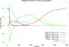 |
Fig. 1 Weights computed by estimator aggregation. |
Parameters of the local and multiscale mixture model used in LGMCA and PolGMCA.
3. Numerical experiments
3.1. Simulations and experimental protocol
Simulations
By the end of 2015, the Planck satellite will provide the finest observations of the polarized sky in the frequency range 30–353 GHz. We naturally propose evaluating the proposed component separation method with simulated polarized Planck data. For that purpose, we will make use of simulations generated with the Planck Sky Model (PSM)1 in Delabrouille et al. (2013).
PSM simulations.
The PSM includes the best of the current knowledge of most polarized astrophysical signals and foregrounds, as well as simulated instrumental noise and beams. In detail, the simulations were obtained using the publicly available PSM version 1.7.8 with the following details.
-
Frequency channels: the simulated data are composed of the seven LFI and HFI channels at frequencies of 33,44,70,100,143,217, and 353 GHz. The frequency-dependent beams are perfect isotropic Gaussian PSFs with a FWHM ranging from 5 arcmin at 217 and 353 GHz to 33 arcmin at 33 GHz. These simulations do not account for the effect of the scanning strategy adopted by full-sky surveys; indeed, these survey strategies are similar to producing non-isotropic and spatially varying beams, which are more elongated in the scanning directions.
-
Instrumental noise: the sky coverage is not uniform and homogeneous, since some areas are more frequently observed than others. The noise statistics (i.e., noise variance map for each frequency channel) are assumed to be known accurately and consistent of the Planck noise variance maps. The simulations account for the inhomogeneity of the noise statistics, but not for its correlation along the scanning direction. Noise is assumed to be uncorrelated.
-
Cosmic microwave background: the CMB map is a correlated random Gaussian realization entirely characterized by its T,E, and B power spectrum and T-E cross-spectrum. In the simulations, the CMB intensity and polarization power spectra and cross-spectra are generated according to the Λ-CDM model derived from the Planck 2013 results. The simulated CMB is Gaussian, and no non-Gaussianity (e.g., lensing, ISW, fNL) has been added. The simulated polarized CMB maps are free of B mode.
-
Point sources: infrared and radio sources were added based on existing catalogs at that time. In the PSM, polarized point sources are attributed a random polarization degree and uniformly random polarization angle.
The Galactic polarization models, which are composed of the dust and synchrotron emissions. These emissions are based on the PSM mamd2008 model Miville-Deschênes et al. (2008) that is parameterized by the intrinsic polarization fraction. By default, it is set to 15% to match the WMAP data.
More precisely,
-
Polarized dust emissions: the polarization of Galactic thermal dust emission is due to the partial alignment of elongated dust grains with the Galactic magnetic field. It is poorly known, however; the current PSM simulations are an extrapolation from the thermal dust intensity. The emission of the thermal dust is modeled by a graybody emission law. PSM simulations have been shown to agree well with the Archeops observations of polarized dust (Ponthieu et al. 2005) and WMAP 94 GHz measurements.
-
Polarized synchrotron emission: the polarized synchrotron emission is obtained by extrapolating WMAP 23 GHz Q and U maps using the same power-law model as for the temperature map. This approach has been shown to be consistent with the WMAP polarized synchrotron maps (Gold et al. 2011).
Comparison protocol.
So far, the component separation methods used to estimate CMB polarization maps are limited to ILC-based techniques (Basak & Delabrouille 2012a) and an extension of SMICA to polarization (Aumont & Macías-Pérez 2007). In contrast to LGMCA, none of these codes is publicly available. The recent analysis of the Planck PR1 temperature data (Planck Collaboration XII 2014) revealed that ILC-based component separation techniques, and especially their harmonic variant, provided some of the best results in the noise-dominant regime: the SMICA map has been obtained by applying harmonic ILC (HILC) for ℓ> 1500. Hence, it is very likely that similar results will hold true in the case of polarization. Consequently, this section focuses on comparing the CMB map derived from HILC (described in Appendix A) and the new PolGMCA method, which combines HILC with the updated version of the LGMCA algorithm.
 |
Fig. 2 Estimated CMB Q maps at 1 deg resolution: Input CMB (left), HILC (middle), and PolGMCA (right). |
 |
Fig. 3 Estimated CMB U maps at 1 deg resolution: Input CMB (left), HILC (middle), and PolGMCA (right). |
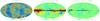 |
Fig. 4 Foreground residual in the estimated Q maps at 1 deg resolution: input CMB (left), HILC (middle), and PolGMCA (right). |
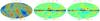 |
Fig. 5 Foreground residual in the estimated U maps at 1 deg resolution: input CMB (left), HILC (middle), and PolGMCA (right). |
The LGMCA algorithm requires defining three parameters: i) the number of sources is set to be equal to the number of channels; ii) the common resolution; and iii) the nominal patch size. All these parameters are given in Table 1 and are chosen as in Bobin et al. (2014b).
3.2. CMB map estimates
Figures 2 and 3 display the estimated CMB Q and U maps, which were computed with HILC and PolGMCA. The maps were smoothed at a resolution of one degree so as to better highlight the large-scale residual features and remove high-frequency noise, thus facilitating visual inspection. These figures first show that the proposed PolGMCA algorithm achieves a much better cleaning of the Galactic center; the HILC map clearly contains significant large-scale foreground residuals, which are mainly limited to the Galactic center. However, while showing fewer residuals in the Galactic center, the PolGMCA map seems to be slightly more contaminated by instrumental noise, as seen from the apparently stronger background fluctuations. To a lesser extent, the same conclusions can be drawn from the estimated U map features in Fig. 3.
Figure 4 shows the total foreground residuals that contaminate the estimated CMB Q maps. These maps were obtained by applying the unmixing parameters to the input foregrounds. These maps were furthermore smoothed to a common resolution of one degree. Both HILC and PolGMCA visually yield low levels of foreground residuals at large Galactic latitudes. As noted earlier in this paragraph, the PolGMCA algorithm achieves a significantly better foreground cleaning in the vicinity of the Galactic center.
Total foreground residualIn this section, we evaluate the quality of estimating the polarized CMB E maps, which we computed with HILC and PolGMCA. The purpose of this article is of course to provide a component separation methods that provides clean, low-foreground, polarized CMB maps at high Galactic latitudes as well as in the Galactic center. For this purpose, the power spectra of the individual and total foreground residuals were computed from various values of the sky coverage –25%, 55%, and 85% – and without any masking (full-sky). These masks are common to all the methods; they were computed based on the foreground residuals of both the two maps so as not to favor or penalize one of these maps. Since these comparisons are based on simulations, the noise and CMB angular power spectra are the actual spectra of the input simulation; they are therefore not based on Monte Carlo simulations. Furthermore, these angular power spectra are displayed with 3σ error bars based on 100 noise simulations. Because the instrumental noise is one of the maing contaminants of the estimated polarized CMB maps, the uncertainties with respect to noise allow assessing the statistical significance of the foreground residuals quite accurately.
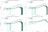 |
Fig. 6 Total foregrounds – top left panel: power spectrum of total foreground residuals for the E map from a sky coverage of 25%. Top right panel: the same from a sky coverage of 55%. Bottom left panel: the same from a sky coverage of 85%. Bottom right panel: the same for the full sky. |
Figure 6 displays the power spectrum of the total foreground residual (i.e., synchrotron, thermal dust, and point sources) for HILC and PolGMCA for various values of the sky coverage. At large scales, for ℓ< 100, the PolGMCA algorithm provides a lower level of foreground residuals whether it is at high Galactic latitudes (sky coverage of 25%) or on the Galactic center (full-sky estimate). This enhancement is very likely the consequence of the new separation mechanism described in Sect. 2.3, which makes the estimation of the E CMB map less sensitive to chance correlations, but at the cost of an increase in the noise level.
At intermediate scales – for 100 <ℓ< 600 – PolGMCA and HILC provide very similar results on 55% of the sky. HILC seems to perform slightly better for high Galactic latitudes. Both methods yield estimates with very low foreground residuals at high Galactic latitudes, which are about one order of magnitude lower than both the noise and the cosmological signal. For a more extended sky coverage, the level of foreground residuals rapidly increases in the CMB E map delivered by the HILC algorithm, while PolGMCA produces a clean full-sky estimate of the E map at intermediate scales. At smaller scales – ℓ> 600 – PolGMCA performs better than HILC with similar noise level but lower foreground residuals. Interestingly, at very large scales – ℓ< 10 – the level of foregrounds is significantly lower than the level of CMB; this suggests that large-scale anomalies in polarization could also be carried out without masking, similarly to what has been done for the temperature large-scale anomaly studies (Rassat et al. 2014). This result makes PolGMCA a good candidate for analyzing the large-scale anomalies of the CMB map.
Figure 6 displays 3σ error bars based on 100 noise simulations, which first reveal that outside the Galactic center (i.e., for masks larger than 85%) the discrepancy between these two methods is not significant with respect to noise uncertainty. In contrast, when no mask is applied, the improvements achieved by the PolGMCA algorithm are statistically significant. This highlights the very good performances of the PolGMCA algorithm in the vicinity of the Galactic center.
Individual foreground residuals. This paragraph investigates the contamination of the polarized CMB map estimates, and especially the CMB E map from individual foregrounds.
-
Thermal dust. Figure 7 features the power spectrum of the residual thermal dust contamination for various sky coverages ranging from 25% to the full sky. For intermediate and small scales (i.e., ℓ> 1000), thermal dust is by far the main contaminant for both the HILC and PolGMCA E maps, whether it is in the Galactic center or at high Galactic latitudes. In this range of multipoles, HILC performs slightly better than PolGMCA for sky coverages smaller than 55%. For larger sky coverage, the ability of PolGMCA to deliver a clean estimate of the CMB map in the Galactic center greatly helps limiting the increase of thermal dust residual from areas close to the Galactic center. It is important to notice that the E map delivered by the PolGMCA algorithm shows a level of thermal dust residual that is about one order of magnitude lower than the level of CMB for ℓ< 1200, even for a sky coverage as high as 85%. At small scales, for ℓ< 100, the CMB E map computed with PolGMCA contains significantly lower thermal dust residuals at all latitudes. HILC provides a slightly lower dust level in the range 100 <ℓ< 1000 at high Galactic latitudes.
-
Synchrotron. The power spectrum of the synchrotron residuals in the HILC and PolGMCA E maps are displayed in Fig. 8. HILC a provides lower synchrotron contamination for ℓ< 20, whether it is in the Galactic center or at higher Galactic latitudes. However, PolGMCA provides significantly lower synchrotron residuals for ℓ> 100, even for high Galactic latitudes.
-
Point sources. Figure 9 shows the power spectrum of the point source contamination. At large scales, PolGMCA exhibits slightly higher point sources residuals for an all-sky coverage. PolGMCA performs slightly better than HILC at intermediate and small scales. It is interesting that that for large sky coverage, the E map obtained with PolGMCA shows a significantly lower level of point source residuals for ℓ> 100; this highlights the ability of the PolGMCA algorithm to remove highly non-Gaussian and non-stationary components such as point sources, especially in the Galactic center. For astrophysical studies, the most prominent point sources will be masked to limit their impact. The level of point source residuals is therefore expected to be significantly lower for both component separation techniques in this setting.
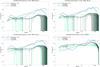 |
Fig. 7 Thermal dust – top left panel: power spectrum of the thermal dust residual in the estimated E map from a sky coverage of 25%. Top right panel: the same from a sky coverage of 55%. Bottom left panel: the same from a sky coverage of 85%. Bottom right panel: the same for the full sky. |
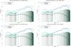 |
Fig. 8 Synchrotron – top left panel: power spectrum of the synchrotron residual in the estimated E map from a sky coverage of 25%. Top right panel: the same from a sky coverage of 55%. Bottom left panel: the same from a sky coverage of 85%. Bottom right panel: the same for the full sky. |
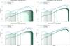 |
Fig. 9 Point sources – top left panel: power spectrum of the point source residuals in the estimated E map from a sky coverage of 25%. Top right panel: the same from a sky coverage of 55%. Bottom left panel: the same from a sky coverage of 85%. Bottom right panel: the same for the full sky. |
3.3. Toward an accurate full-sky estimate of the CMB polarization maps
In this section, we investigate with more precision the quality of estimating the CMB polarization map across the sky. Indeed, one of the objectives of this article is to achieve an accurate full-sky estimate of polarized CMB maps. For this purpose, and following an analysis method we have used before (Bobin et al. 2013a,b, 2014b), the accuracy of a CMB map can be evaluated by computing the level of foreground residuals in bands of latitudes in the wavelet domain. Using wavelets, one can analyze the estimated CMB maps with a good localization in space as well as in harmonic space.
More precisely, the estimated Q and U maps were decomposed into six wavelet bands (see Starck et al. 2006). Each of the six bands was then split uniformly into 18 bands of latitudes; each band of latitude has a width of 10°. Figure 10 reports the energy level (Euclidean norm) of the total foreground residuals (i.e., thermal dust, synchrotron, and point sources) for the six wavelet scales. By convention, the wavelet scale 0 corresponds to the smallest scales (ℓ> 1600) and scale 5 to large scales (50 <ℓ< 100).
It is first interesting to note that at all scales, HILC has a level of foreground residuals that exceeds the level of the CMB in the Galactic center at latitudes of about ±15°. This is precisely in the vicinity of the Galactic center at which the stationarity assumptions, made in the framework of HILC, are probably the least valid and where the use of spatial localization and sparsity is the most beneficial for component separation. Consequently, the CMB map estimated by the PolGMCA algorithm has significantly lower foreground residuals for Galactic latitudes lower than 15°. More precisely, in the Galactic plane, the HILC Q map has an order of magnitude higher foreground residuals than PolGMCA, in wavelet bands corresponding to ℓ> 400.
For the first three wavelet scales, the PolGMCA Q and U maps have a level of foreground residuals that is constantly lower than the level of CMB throughout the sky. At larger scales, the CMB is dominated by the foregrounds only for latitudes that are lower than ±10°.
For Galactic latitudes higher than ±25°, these plots confirm the very good efficiency of the HILC algorithm in regions where instrumental noise is, by far, the most prominent contaminant in the data. The PolGMCA algorithm generally provides similar or slightly higher levels of foregrounds in high Galactic regions, but still much lower than the level of instrumental noise.
These numerical results highlight the efficiency of the proposed PolGMCA algorithm to provide a very accurate estimate the polarized CMB maps in the vicinity of the Galactic center while providing residual levels that are competitive to the very effective HILC algorithm at high Galactic latitudes at intermediate and small scales. The PolGMCA is shown to be particularly effective at large scales (i.e., for ℓ< 200), where it yields estimates of the CMB Q and U maps with significantly lower levels of total foreground at all Galactic latitudes.
 |
Fig. 10 Total foreground residuals in the Stokes parameter Q map: mean squared error (MSE) per band of latitude in the wavelet domain. Dashed lines represent the noise level for each component separation method. |
 |
Fig. 11 Total foregrounds residuals in the Stokes parameter U map: mean squared error (MSE) per band of latitude in the wavelet domain. Dashed lines represent the noise level for each component separation method. |
4. Conclusion
We presented a novel component separation method that is dedicated to estimating the CMB polarization modes. This approach builds upon the GMCA algorithm, which emphasizes the sparsity of the sought-after sources in the wavelet domain to separate them out. The proposed algorithm, dubbed PolGMCA, extends the basic GMCA algorithm with two significant improvements: i) it allows for the efficient separation of partially correlated sources thanks to recent improvements of the GMCA algorithm; and ii) it aggregates sparse and second-order based CMB estimators to benefit from their complementary characteristics in terms of propagated noise and foreground residuals. Subsequently, we showed that the proposed PolGMCA algorithm exhibits the following interesting properties:
-
It provides an improved estimate of the polarized CMB maps particularly at large scales, typically for ℓ< 200, outside the Galactic center, where the ability to account for the partial correlation the components is essential. However, these improvements are not significant with respect to the noise-related uncertainty.
-
It provides very accurate estimates of the polarized CMB maps in regions where foregrounds, which are by nature non-Gaussian and non-stationary, dominate. This is specifically the case in the vicinity of the Galactic center at latitudes ±15°. In this setting, the PolGMCA algorithm benefits by a large amount from its ability to account for the partial correlation of the components to be removed.
-
In noise-dominated regions of the sky, the polarized CMB maps provided by the PolGMCA algorithm have foreground levels that are close to the HILC algorithm, which is assumed to be close to optimality in this noise regime.
Altogether, these results make the PolGMCA algorithm a good candidate for Galactic studies in polarization, studying large-scale anomalies, and testing the detection of B-modes from Planck data.
For more details about the PSM, we refer to the PSM website: http://www.apc.univ-paris7.fr/~delabrou/PSM/psm.html
Acknowledgments
This work is supported by the European Research Council grant SparseAstro (ERC-228261) and partially by the French National Agency for Research (ANR) 11-ASTR-034-02-MultID. We used the Healpix software (Gorski et al. 2005) and the iSAP2 software.
References
- Aiola, S., Kosowsky, A., & Wang, B. 2015, Phys. Rev. D, 91, 043510 [NASA ADS] [CrossRef] [Google Scholar]
- Aumont, J., & Macías-Pérez, J. F. 2007, MNRAS, 376, 739 [NASA ADS] [CrossRef] [Google Scholar]
- Basak, S., & Delabrouille, J. 2012a, ArXiv e-prints [arXiv:1204.0292] [Google Scholar]
- Basak, S., & Delabrouille, J. 2012b, MNRAS, 419, 1163 [NASA ADS] [CrossRef] [Google Scholar]
- Ben-David, A., & Kovetz, E. 2014, MNRAS, 445, 2116 [NASA ADS] [CrossRef] [Google Scholar]
- Bennett, C. L., Banday, A. J., Gorski, K. M., et al. 1996, ApJ, 464, L1 [NASA ADS] [CrossRef] [Google Scholar]
- Bennett, C. L., Larson, D., Weiland, J. L., et al. 2013, ApJS, 2031, 20 [NASA ADS] [CrossRef] [Google Scholar]
- BICEP2/Keck, P. C. 2015, Phys. Rev. Lett., 114, id. 101301 [Google Scholar]
- Bobin, J., Starck, J.-L., Sureau, F., & Basak, S. 2013a, A&A, 550, A73 [NASA ADS] [CrossRef] [EDP Sciences] [Google Scholar]
- Bobin, J., Sureau, F., Paykari, P., et al. 2013b, A&A, 553, L4 [NASA ADS] [CrossRef] [EDP Sciences] [Google Scholar]
- Bobin, J., Rapin, J., Starck, J.-L., & Larue, A. 2014a, in Proc. IEEE ICIP, 4 [Google Scholar]
- Bobin, J., Sureau, F., Starck, J.-L., Rassat, A., & Paykari, P. 2014b, A&A, 563, A105 [NASA ADS] [CrossRef] [EDP Sciences] [Google Scholar]
- Cardoso, J., Snoussi, H., Delabrouille, J., & Patanchon, G. 2002, in Proc. EUSIPCO’02 [arXiv:astroph/0209469] [Google Scholar]
- Comon, P., & Jutten, C. 2010, Handbook of blind source separation (Elsevier), 2 [Google Scholar]
- Delabrouille, J., Cardoso, J.-F., & Patanchon, G. 2003, MNRAS, 346, 1089 [NASA ADS] [CrossRef] [Google Scholar]
- Delabrouille, J., Betoule, M., Melin, J.-B., et al. 2013, A&A, 553, A96 [NASA ADS] [CrossRef] [EDP Sciences] [Google Scholar]
- Eriksen, H. K., Banday, A. J., Gorski, K. M., & Lilje, P. B. 2004, ApJ, 612, 633 [NASA ADS] [CrossRef] [Google Scholar]
- Eriksen, H. K., Jewell, J. B., Dickinson, C., et al. 2008, ApJ, 676, 663 [Google Scholar]
- Fernández-Cobos, R., Vielva, P., Barreiro, R. B., & Martínez-González, E. 2012, MNRAS, 420, 2162 [NASA ADS] [CrossRef] [Google Scholar]
- Flauger, R., Hill, J., & Spergel, D. N. 2014, J. Cosmol. Astropart. Phys., 39 [Google Scholar]
- Gold, B., Odegard, N., Weiland, J. L., et al. 2011, ApJS, 192, 15 [Google Scholar]
- Gorski, K., Hivon, E., Banday, A. J., et al. 2005, ApJ, 622, 11 [NASA ADS] [Google Scholar]
- Hu, W., & White, M. 1997, New Astron., 2, 1 [Google Scholar]
- Kim, J., Naselsky, P., & Christensen, P. 2009, Phys. Rev. D., 79 [Google Scholar]
- Lanusse, F., Paykari, P., Starck, J., et al. 2014, A&A, 571, A1 [NASA ADS] [CrossRef] [EDP Sciences] [Google Scholar]
- Leach, S. M., Cardoso, J.-F., Baccigalupi, C., et al. 2008, A&A, 491, 597 [NASA ADS] [CrossRef] [EDP Sciences] [Google Scholar]
- Masi, S., Ade, P., Bock, J., et al. 2006, A&A, 458, 687 [NASA ADS] [CrossRef] [EDP Sciences] [Google Scholar]
- Miville-Deschênes, M.-A., Ysard, N., Lavabre, A., et al. 2008, A&A, 490, 6 [Google Scholar]
- Mortonson, M., & Seljak, U. 2014, J. Cosmol. Astropart., 1410, 1 [Google Scholar]
- Planck Collaboration Int. XXXII. 2014, A&A, accepted, DOI: 10.1051/0004-6361/201425044 [Google Scholar]
- Planck Collaboration XII. 2014, A&A, 571, A12 [NASA ADS] [CrossRef] [EDP Sciences] [Google Scholar]
- Planck Collaboration IX. 2015, A&A, submitted [arXiv:1502.05956] [Google Scholar]
- Planck Collaboration XIII. 2015, A&A, submitted [arXiv:1502.01589] [Google Scholar]
- Ponthieu, N., Macías-Pérez, J. F., Tristram, M., et al. 2005, A&A, 444, 327 [NASA ADS] [CrossRef] [EDP Sciences] [Google Scholar]
- Rassat, A., Starck, J.-L., Paykari, P., Sureau, F., & Bobin, J. 2014, J. Cosmol. Astropart., 6 [Google Scholar]
- Readhead, A. C. S., Myers, S. T., Pearson, T., et al. 2004, Science, 306, 1 [Google Scholar]
- Starck, J.-L., Moudden, Y., P., A., & Nguyen, M. 2006, A&A, 446, 1191 [NASA ADS] [CrossRef] [EDP Sciences] [Google Scholar]
- Starck, J., Moudden, Y., & Bobin, J. 2009, A&A, 497, 931 [NASA ADS] [CrossRef] [EDP Sciences] [Google Scholar]
- Sunyaev, R. A., & Zeldovich, Y. B. 1970, Astrophys. Space Sci., 7, 3 [Google Scholar]
- Tegmark, M., de Oliveira-Costa, A., & Hamilton, A. 2003, ApJ, 68, 12 [Google Scholar]
- Yang, Y. 2004, Bernoulli, 10, 25 [CrossRef] [Google Scholar]
- Zaldarriaga, M. 1998, ApJ, 503, 1 [NASA ADS] [CrossRef] [Google Scholar]
Appendix A: Harmonic ILC implementation
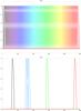 |
Fig. A.1 Bands of multipoles used to derive HILC weights: left all the 81 overlapping bands used to compute the ILC weights in the harmonic domain. Right: examples of five different bands for better visualization. |
Harmonic ILC has been widely used, mainly to estimate CMB maps from WMAP data in temperature data (Tegmark et al. 2003) and polarization (Kim et al. 2009). More recently, the SMICA CMB polarized maps derived from the Planck PR2 data (Planck Collaboration IX 2015) are equivalent to a HILC solution at high ℓ multipoles. The appeal of HILC resides in its ability to precisely account for the different beams at each channel as well as in its accuracy in modeling stationary Gaussian random fields such as the CMB.
In this paper, and inspired by Tegmark et al. (2003), Kim et al. (2009), we implemented an HILC method that proceeds in two steps:
-
Fitting the ILC weights: ILC estimates weights to obtain a minimum variance solution. In the case of HILC, this step is performed independently on overlapping bands of multipoles that span the desired range of multipoles [0,2500]. The bands have a fixed width Δ = 80; this width was tuned so as to provide the best estimation accuracy in PSM simulations, as a trade-off between good foreground modeling (narrow bands) and statistical robustness (broad bands). All the 81 bands used to derive ILC weights are displayed in the left panel of Fig. A.1. Let bi,ℓ be the beam of the ith frequency channel, wl,ℓ be the filter defining the lth band, and
 be the aℓ,m coefficient of the ith frequency channel, the weights [πi,l] i = 1,...,M in the lth band are computed by minimizing the following problem:
  (A.1)
(A.1) -
Derivingℓ-dependent weights: from the 81 bands, one derives the weight per band and observation. A simple interpolation procedure was used so as to derive a weight per ℓ and per observation i. This interpolation step was performed to provide weight vectors πi = [πi(0),...,πi(ℓ),...,πi(ℓmax)] as follows:
 (A.2)which is essentially a simple interpolation by weighted averaging, where the filters wl were used as weights.
The exact same HILC algorithm is used to aggregate the CMB estimators in the PolGMCA algorithm described in Sect. 2.
All Tables
All Figures
|
Fig. 1 Weights computed by estimator aggregation. |
| In the text | |
|
Fig. 2 Estimated CMB Q maps at 1 deg resolution: Input CMB (left), HILC (middle), and PolGMCA (right). |
| In the text | |
|
Fig. 3 Estimated CMB U maps at 1 deg resolution: Input CMB (left), HILC (middle), and PolGMCA (right). |
| In the text | |
|
Fig. 4 Foreground residual in the estimated Q maps at 1 deg resolution: input CMB (left), HILC (middle), and PolGMCA (right). |
| In the text | |
|
Fig. 5 Foreground residual in the estimated U maps at 1 deg resolution: input CMB (left), HILC (middle), and PolGMCA (right). |
| In the text | |
|
Fig. 6 Total foregrounds – top left panel: power spectrum of total foreground residuals for the E map from a sky coverage of 25%. Top right panel: the same from a sky coverage of 55%. Bottom left panel: the same from a sky coverage of 85%. Bottom right panel: the same for the full sky. |
| In the text | |
|
Fig. 7 Thermal dust – top left panel: power spectrum of the thermal dust residual in the estimated E map from a sky coverage of 25%. Top right panel: the same from a sky coverage of 55%. Bottom left panel: the same from a sky coverage of 85%. Bottom right panel: the same for the full sky. |
| In the text | |
|
Fig. 8 Synchrotron – top left panel: power spectrum of the synchrotron residual in the estimated E map from a sky coverage of 25%. Top right panel: the same from a sky coverage of 55%. Bottom left panel: the same from a sky coverage of 85%. Bottom right panel: the same for the full sky. |
| In the text | |
|
Fig. 9 Point sources – top left panel: power spectrum of the point source residuals in the estimated E map from a sky coverage of 25%. Top right panel: the same from a sky coverage of 55%. Bottom left panel: the same from a sky coverage of 85%. Bottom right panel: the same for the full sky. |
| In the text | |
|
Fig. 10 Total foreground residuals in the Stokes parameter Q map: mean squared error (MSE) per band of latitude in the wavelet domain. Dashed lines represent the noise level for each component separation method. |
| In the text | |
|
Fig. 11 Total foregrounds residuals in the Stokes parameter U map: mean squared error (MSE) per band of latitude in the wavelet domain. Dashed lines represent the noise level for each component separation method. |
| In the text | |
|
Fig. A.1 Bands of multipoles used to derive HILC weights: left all the 81 overlapping bands used to compute the ILC weights in the harmonic domain. Right: examples of five different bands for better visualization. |
| In the text | |
Current usage metrics show cumulative count of Article Views (full-text article views including HTML views, PDF and ePub downloads, according to the available data) and Abstracts Views on Vision4Press platform.
Data correspond to usage on the plateform after 2015. The current usage metrics is available 48-96 hours after online publication and is updated daily on week days.
Initial download of the metrics may take a while.