| Issue |
A&A
Volume 582, October 2015
|
|
|---|---|---|
| Article Number | A9 | |
| Number of page(s) | 9 | |
| Section | Extragalactic astronomy | |
| DOI | https://doi.org/10.1051/0004-6361/201526596 | |
| Published online | 29 September 2015 | |
Restarting radio activity and dust emission in radio-loud broad absorption line quasars
1 Max-Planck Institute for Radio Astronomy, Auf dem Hügel 69, 53121 Bonn, Germany
e-mail: This email address is being protected from spambots. You need JavaScript enabled to view it.
2 INAF–Istituto di Radioastronomia, via P. Gobetti 101, 40129 Bologna, Italy
3 European Southern Observatory, Alonso de Córdova 3107, Vitacura, Casilla 19001, Santiago de Chile, Chile
4 Netherlands Institute for Radio Astronomy, Postbus 2, 7990 AA Dwingeloo, The Netherlands
5 Kapteyn Astronomical Institute, Rijksuniversiteit Groningen, Landleven 12, 9747 AD Groningen, The Netherlands
6 Instituto de Física de Cantabria (CSIC-Universidad de Cantabria), Avda. de los Castros s/n, 39005 Santander, Spain
Received: 25 May 2015
Accepted: 29 July 2015
Abstract
Context. Broad absorption line quasars (BAL QSOs) are objects that show absorption from relativistic outflows that have velocities up to 0.2c. In about 15% of quasars, these manifest as absorption troughs on the blue side of UV emission lines, such as C iv and Mg ii. The launching mechanism and duration of these outflows is not clear yet.
Aims. In this work, we complement the information collected in the cm band for our previously presented sample of radio loud BAL QSOs (25 objects with redshifts 1.7 < z < 3.6) with new observations in the m and mm bands. Our aim is to verify the presence of old, extended radio components in the MHz range and probe the emission of dust (linked to star formation) in the mm domain.
Methods. We observed 5 sources from our sample, which already presented hints of low-frequency emission, with the GMRT at 235 and 610 MHz. Another 17 sources (more than half the sample) were observed with bolometer cameras at IRAM-30 m (MAMBO2, 250 GHz) and APEX (LABOCA and SABOCA, 350 and 850 GHz, respectively).
Results. All sources observed with the GMRT present extended emission on a scale of tens of kpc. In some cases these measurements allow us to identify a second component in the SED at frequencies below 1.4 GHz, beyond the one already studied in the GHz domain. In the mm band, only one source shows emission clearly ascribable to dust, detached from the synchrotron tail. Upper limits were obtained for the remaining targets.
Conclusions. These findings confirm that BAL QSOs can also be present in old radio sources or even in restarting ones where favourable conditions for the outflow launching or acceleration are present. A suggestion that these outflows could be precursors of the jet comes from the possibility that ~70% of our sample is in a GigaHertz Peaked Spectrum (GPS) or Compact Steep Spectrum (CSS)+GPS phase. This would confirm the idea proposed by other authors that these outflows could be recollimated to form the jet. Compared with previous works in the literature, dust emission seems to be weaker than what is expected in “normal” QSOs (both radio loud and radio quiet ones), suggesting that a feedback mechanism could inhibit star formation in radio-loud BAL QSOs.
Key words: quasars: absorption lines / galaxies: active / galaxies: evolution / radio continuum: galaxies
© ESO, 2015
1. Introduction
In the context of active galactic nuclei (AGNs), outflows from the central region are commonly detected as absorption lines in more bands. In the UV and optical ranges, they can be present in ~70% of type 1 AGNs, with an extension up to kpc scales and velocities up to ~1000 km s-1 (Harrison et al. 2014). A similar percentage (~60%) has been found in the quasar (QSO) population (Ganguly & Brotherton 2008). In the X-ray band, more highly ionised outflows are detected as ultra fast outflows (UFO) both in radio-quiet (RQ; Pounds et al. 2003) and radio-loud (RL) AGNs (Tombesi et al. 2014) with much higher velocities in the range 0.03–0.4c. A feedback effect from outflows on the host galaxy has been proven by different authors in recent years (e.g. Feruglio et al. 2010; Wang et al. 2010; Sturm et al. 2011), and lately they have been proven to hamper star formation (Tombesi et al. 2015).
Broad absorption line quasars (BAL QSOs) are among the objects that present the fastest outflows. These are detected in about 15% of QSOs as broad absorption troughs in the UV spectrum on the blue side of emission lines from ionised species, mainly C iv and Mg ii. They can be both detached or superimposed on the emission peak and can reach relativistic velocities of up to 0.2c (Hewett & Foltz 2003). Allen et al. (2011) have found a dependence with redshift of the BAL fraction, decreasing a factor of 3.5 ± 0.4 from z ~ 4 to ~2. The mechanism at the origin of these violent outflows has not been unveiled yet. The two main scenarios discussed in the literature tend to ascribe the BAL phenomenon to: 1) young objects, in which the strong nuclear starburst activity is still expelling a dust cocoon (Briggs et al. 1984; Sanders 2002; Farrah et al. 2007); or 2) normal QSOs, whose outflows intercept the line of sight of the observer (Elvis 2000). In this case, relativistic outflows are supposed to be commonly present in QSOs, but detected only when orientation is favourable. The variability of the BAL troughs has been explored by many authors in past years, thanks to the increase in available spectroscopic surveys data (Gibson et al. 2008, 2010; Capellupo et al. 2011, 2012; Vivek et al. 2012) and a typical duty cycle of about a thousand years for the BAL-producing outflow has been found (Filiz Ak et al. 2012, 2013).
Several works have been published recently that try to collect information in the different electromagnetic bands. In particular, the emission in the radio band has been used to probe the orientation and age of these objects (Montenegro-Montes et al. 2008; DiPompeo et al. 2011; Bruni et al. 2012, 2013). No clear hints of a favoured scenario were found in these works, resulting in indications of different possible orientations and different ages for RL BAL QSOs. In this work, we present follow-up observations of sources from our previously studied sample (Bruni et al. 2012). We explored the emission properties at m and mm wavelengths to complement the multi-wavelength view of these objects, which have already been studied in the cm band in our previous work.
The detection of a strong MHz emission can be safely interpreted as the presence of old extended radio plasma connected to a former AGN radio-active phase, which can be as old as 107–108 yr (Konar et al. 2006, 2013). It has been shown that jets in RL AGNs can indeed have multiple phases of activity (Lara et al. 1999; Schoenmakers et al. 2000; Saikia & Jamrozy 2009; Nandi et al. 2014) with a duty cycle that depends on the source radio power (Best et al. 2005; Shabala et al. 2008). Hints of these components in BAL QSOs have already been found from literature data for the same sample studied in this paper and was presented in Bruni et al. (2012). This kind of emission adds a significant amount of information within the framework of the presented models for BAL QSOs. In particular, if the young scenario was the most realistic one, no further components than the one peaking in the MHz–GHz range should be present, since GigaHertz-Peaked Spectrum sources (GPS) and Compact Steep Spectrum sources (CSS, O’Dea 1998), together with high frequency peakers (HFP, Dallacasa et al. 2000) are among the youngest radio sources.
To date, systematic searches of diffuse emission around GPS and CSS sources find about 20% detections (Stanghellini et al. 1990, 2005). In light of this, we use low-frequency GMRT observations to probe possible extended emission around BAL QSO with the aim of possibly confirming or discarding the youth scenario described in the previous paragraph. The radio phase itself does not seem to introduce significant differences in RL BAL QSOs with respect to RQ ones (Bruni et al. 2014; Rochais et al. 2014), so it is a valid tool for studying the general phenomenology of these objects.
The continuum emission of dust in the rest-frame far-infrared domain (FIR) can be detected at mm wavelengths (over 100 GHz) for objects with z ~ 2. Objects enshrouded by gas and dust can host star formation regions (Zahid et al. 2014), and thus show high star formation rates that may indicate a young age of the galaxy. A flux density excess in the FIR could be an indicator of a different age for BAL QSOs with respect to the non-BAL QSO population, and thus help in distinguishing between the orientation and the evolutionary models. There are two major works presenting (sub-)mm observations on samples of BAL QSOs. Willott et al. (2003) showed SCUBA measurements on a sample of 30 RQ BAL QSOs and conclude that there is no difference between BAL QSOs and a comparison sample of non-BAL QSOs. Nevertheless, based on SCUBA observations of 15 BAL QSOs, Priddey et al. (2007) found tentative evidence for a dependence of sub-mm flux densities on the equivalent width of the characteristic C iv BAL, which “suggests that the BAL phenomenon is not a simple geometric effect [...] but that other variables, such as evolutionary phase, [...] must be invoked”. Cao Orjales et al. (2012) discuss the far-infrared properties and star formation rates (SFR) of BAL QSOs (without distinguishing between RL and RQ ones), using data from the Herschel-ATLAS project. They find no differences with respect to non-BAL QSOs, concluding that a scenario in which BAL QSOs are objects expelling a dust cocoon is improbable.
The main difference between the above samples and our target sample is the radio loudness of our sources. With the radio data presented in Bruni et al. (2012) we were able to characterise the synchrotron spectra of our sources and thus to study the peak frequency and spectral index distributions with respect to the “normal” QSO population. An upper limit to the synchrotron emission at mm wavelengths can also be constrained.
A search for HFP, which is the youngest known radio sources with the highest turnover frequencies, shows only a very low percentage of sources with peak frequencies close to 20 GHz (Dallacasa et al. 2000), with the most extreme case at 25 GHz leading to a formal age of only some 50 yr (Orienti & Dallacasa 2008). As any upturn towards an even higher peak frequency would be visible in our spectral energy distributions (SEDs), we can safely assume that the extrapolated synchrotron emission reflects its true contribution at 250 GHz and that any observed excess emission can be attributed to the presence of cold dust. Moreover, the variability study presented in Bruni et al. (2012) excludes any possibly significant variability even at high frequencies on a three-year time scale for this sample of objects.
The outline of the paper is as follows. In Sect. 2 we describe the BAL QSO sample. The radio observations are reported in Sect. 3. In Sect. 4 we present the results concerning morphology at MHz frequencies and dust abundance. Section 5 offers a discussion of the results in the context of recent works about BAL QSOs.
The cosmology adopted throughout the work assumes a flat universe and the following parameters: H0 = 71 km s-1 Mpc-1, ΩΛ = 0.73, ΩM = 0.27.
2. The RL BAL QSO sample
The radio-loud BAL QSO sample studied in this paper is presented in Bruni et al. (2012). All sources were chosen among objects from the fourth edition of SDSS Quasar Catalogue (Schneider et al. 2007), drawn from the fifth data release of the Sloan Digital Sky Survey (SDSS-DR5; Adelman-McCarthy et al. 2007). To select RL objects, we cross-matched the SDSS with the FIRST (Faint Images of the Radio Sky at Twenty-cm; Becker et al. 2001), and only those with a counterpart lying <2 arcsec away and having S1.4 GHz> 30 mJy were considered. All of these satisfy the radio-loudness definition by Stocke et al. (1992). Moreover, the selection has been limited to those objects whose redshifts lie in the range 1.7 <z< 4.7, allowing the identification of both C iv and Mg ii absorption features on SDSS spectra. To select genuine BAL QSOs, only objects with an absorption index of (AI) > 100 km s-1 were considered, and only troughs broader than 1000 km s-1 were used for this calculation1. This resulted in 25 RL BAL QSOs. For a complete description of the sample and the selection procedure, refer to Bruni et al. (2012).
Summary of the observations and setups presented in this paper.
3. Radio observations and data reduction
This paper presents observations that complement the ones performed by Bruni et al. (2012) at cm wavelengths. The GMRT, the APEX single-dish, and the IRAM 30-m telescope were used to extend the available SEDs extension. Table 1 summarises the different runs and observing setups.
3.1. Giant Metrewave Radio Telescope
Observations at frequencies of 235 MHz and 610 MHz with the GMRT were performed for five sources during January 2010. We used the double frequency mode to observe simultaneously at the two frequencies. The total bandwidth for each band was 33 MHz, divided into 256 channels of 0.13 MHz each. We observed in snapshot mode to improve the UV coverage for the sources. Standard phase and amplitude were calibrated with 3C 286 as primary calibrator about every four hours and suitable phase calibrators near targets every ~30 min. Correlation used the GSB software correlator at NCRA. Data were reduced with the AIPS2 package with the standard procedures. Flux densities were extracted from images via Gaussian fit of the components, using task JMFIT inside AIPS.
3.2. IRAM-30 m single dish
We could observe 11 sources of the BAL QSO sample at 250 GHz with the IRAM-30 m telescope, during the 2010 summer pool session. We used the MAMBO2 117-pixel bolometer in ON/OFF mode, since all of our sources are point-like for this telescope (HPBW = 11 arcsec). With average atmospheric conditions, the detector could reach a noise of ~1 mJy/beam in ~40 min of observing time. We observed each source for this duration in order to obtain a detection or a 3σ upper limit. Skydip, calibration, and pointing scans were regularly performed during the runs, and each time the observing direction in the sky changed significantly in elevation. Focus was repeated at sunrise and sunset. A standard reduction used the MOPSIC3 script provided by IRAM.
3.3. APEX
From 2010 to 2012 we observed with APEX a total of nine southern sources from the BAL QSO sample. All of them were observed with the SABOCA bolometer array (Siringo et al. 2010) at 850 GHz in photometry mode (HPBW ~ 8 arcsec) and two of the sources (0044+00 and 1404+07) also in mapping mode. In addition, one of the sources (0044+00) was observed with the LABOCA bolometer array (Siringo et al. 2009) at 345 GHz in photometry mode (HPBW ~ 19 arcsec). APEX observations were carried out in service mode with typical integration times of 1 h per source, in order to reach rms values around 20 mJy/beam. Calibration was based on observations of primary calibrators (Mars and Uranus), as well as on skydips measured at the same azimuth of the targets to derive atmospheric opacity. A standard reduction was done using the version 2.15–1 of the CRUSH4 software, which offers an improved pipeline for photometric data as compared to earlier versions.
3.4. Error determination
In the flux-density error calculation, different contributions were considered for the GMRT interferometric observations:
-
the thermal noise, ΔSnoise, which is estimated from the map, in empty regions of sky surrounding the target;
-
the fractional calibration error, ΔScalib, estimated as the visibilities dispersion of the unresolved flux-density calibrators.
In particular, we followed the approach proposed by Klein et al. (2003). The expression used is 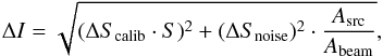 (1)where Abeam and Asrc are the area of the synthesised beam and the aperture used to extract the source flux density, respectively. From their ratio we determined the number of beams contained in the source.
For APEX and IRAM-30 m data, obtained with bolometer receivers, the error was calculated using the respective packages for data reduction, estimating the noise from off-source subscans.
3.5. The polarimetry campaign
During 2011, we conducted a polarimetry campaign using the EVLA and the Effelsberg-100 m single dish on this same sample to implement data later presented in Bruni et al. (2012) and to probe the polarisation of the faintest sources with deeper observation. The results from this campaign will be presented in a future paper, but we decided to use part of the obtained total flux-density measurements to improve the SED coverage of this work (see Table 2). Also, one of the sources observed with the EVLA turns out to have a resolved structure (0849+27), and we present here the map (see Sect. 4.1). This same source was also observed during our mm campaign (see Table 4). Observations and data reduction were conducted as in Bruni et al. (2012).
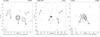 |
Fig. 1 Maps of BAL QSO 0849+27 from the FIRST survey (left panel – 1.4 GHz, beam 5.40 × 5.40 arcsec), our EVLA observations (central panel – 4.86 GHz, beam 1.95 × 1.25 arcsec), and our VLBA observations ((right panel – 5 GHz, beam 2.99 × 1.15 mas). Contours are multiples of 3σ, according to the label. Dashed contours are negative. The synthesised beam size is shown in the lower left corner of each map. The scale of the right panel is in mas. |
Revised flux densities (top lines) and measurements from our polarimetry campaign (bottom lines).
4. Results
In the following, we present the results from our observing campaign: the morphology could be studied with the GMRT interferometer, while images from the IRAM and APEX bolometers were used for photometric measurements. The collected information is presented in Table 3, and SEDs, including flux densities at cm wavelengths from Bruni et al. (2012) and our polarimetry campaign, are presented in Fig. 3 and discussed in Sect. 4.2.
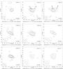 |
Fig. 2 Maps of 5 BAL QSOs observed with the GMRT at 235 and 610 MHz. Contours are multiples of 3σ, according to the label. Dashed contours are negative. The synthesised beam size is shown in the lower left corner of each map. |
Information collected with the GMRT interferometer.
4.1. Morphology
From the GMRT and EVLA maps, we were able to investigate the morphologies of the sources on arcsec scales. The frequency range explored with the GMRT allowed us to put some constraints on the presence of extended, old, radio components.
GMRT maps
With the GMRT, we observed the five sources from our BAL QSO sample showing the strongest low-frequency emission in the flux densities collected from archival survey data. The goal was the detection of extended emission at 235 or 610 MHz, indicating a previous radio-activity period of the central AGN, thus putting a constraint on the age. Maps show components with deconvolved dimensions greater than zero in most cases, corresponding to a fraction of the beam (see Fig. 2). One source (1159+01) presents an elongated structure at 235 MHz, confirmed by the detection of a second component (B) at higher resolution in the 610 MHz map. This structure is compatible with the one seen in the pc-scale maps obtained by Hayashi et al. (2013), where a jet extension at a comparable position angle is visible. This could confirm the presence of two different radio phases on different scales, as also highlighted by the SED of this object (see Sect. 4.2). Quantities for all sources at the two frequencies are presented in Table 3, together with projected linear sizes. When a zero deconvolved size was found, we considered the corresponding beam size as the upper limit. For the only resolved source (1159+01), we give values for both components.
These measurements confirm the presence of a low-frequency, older radio component in some BAL QSOs, thus excluding that they are a subclass of young radio objects. These components are significantly larger in size than the values of a few kpc measured for the high-frequency, unresolved, counterparts (see Bruni et al. 2012), thus suggesting different emitting regions for them both. The flux densities found fit nicely with collected data from surveys (see Fig. 3).
EVLA map of 0849+27
During our polarimetry campaign, we could observe the peculiar BAL QSO 0849+27 with the EVLA at 4.86 GHz. The map of the resolved structure of this source at 1.4 GHz, which was obtained from the FIRST survey, was already presented in a previous work from our group (Bruni et al. 2012). This turned out to be the most extended BAL QSO of our sample (44 arcsec, 382 kpc, between components A and C). We could obtain a map at 4.8 GHz from our subsequent EVLA observation in 2011, taking advantage of the improved performance of this instrument and also of a high resolution (pc-scale) map of the core component from our VLBA programme (see Bruni et al. 2013). Results are presented in Fig. 1.
Four out of five components detected in the FIRST data are visible in our EVLA map (A, B, C, E), while the flux density of component D seems to drop below the 3σ significance level. Total flux densities as measured at 4.86 GHz are 27.6 ± 0.7 mJy, 2.0 ± 0.2 mJy, 0.49 ± 0.05 mJy, and 0.41 ± 0.05 mJy for components A, B, C, E, respectively. Component E was not classified in our previous FIRST map, but given the clear detection we obtained in the EVLA map, we extracted the flux density at the corresponding position in the FIRST map, where a single contour was present. This resulted in 2.36 ± 0.15 mJy. The obtained spectral indexes for these components are − 0.54 ± 0.04, − 1.10 ± 0.17, − 1.78 ± 0.18, and − 1.41 ± 0.22 for components A, B, C, and E, respectively. A flat spectral index (>–0.5) usually identifies the core for non-Doppler-boosted components: component A shows a spectral index compatible with that value within the error, while B, C, and E have a steep spectral index (<–0.5). From our VLBA observations, we could confirm that core is component A, since on the pc scale it shows a core-jet structure, with one of the two components (A1) having a flat spectral index of − 0.12 ± 0.20 between 5 and 8.4 GHz.
The peculiar morphology of this source, explored on both kpc and pc scales, suggests a jet precession or radio-activity phases with different jet axes. In fact, trajectories connecting the core (A) with the other components detected on the kpc scale are all different, not permitting one as the counter jet of the other to be identified. Moreover, the pc-scale structure shows a further launching direction for the most recent component (A2), which does not correspond to any among the ones on the kpc scale. In this scenario, the BAL-producing outflow would be present in a source that presents multiple ongoing radio phases: this would not be easily explicable with the young scenario.
4.2. SEDs shape from 235 MHz to 850 GHz
We present here a study of the SED shape for the objects in this work. We implemented the new flux densities in the ones from Bruni et al. (2012), which spans 74 MHz up to 43 GHz, in order to improve the overall frequency coverage. For three sources (0756+37, 0816+48, 1335+02) we provide a revised flux density for the VLA measurements presented in Bruni et al. (2012): for source 0816+48, during previous data reduction, the vicinity of a strong source led to an incorrect phase referencing, resulting in an overestimated flux density measurement. While our flux-extraction algorithm missed the source for sources 0756+37 and 1335+02, displaced by a few arcsec from the map centre from atmospheric effects. The revised values are given in Table 2.
Results for the 17 BAL QSOs observed in the mm band: 250 GHz flux densities from IRAM-30 m, 345, and 850 GHz from APEX.
Flux densities at mm wavelengths
Flux density from the dust grey-body thermal emission can be described by the following equation (Hughes et al. 1997): 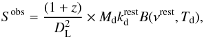 (2)where Sobs is the observed flux density at a given frequency νobs, νrest the rest-frame frequency, DL the luminosity distance, z the target redshift,
  the mass absorption coefficient at a given rest frequency, B the black-body Planck function, Td the dust temperature, and Md the dust mass. Typical AGN values for Td and Md from the most recent works in the literature are 10 <Td< 60 K, and Md ~ 108M⊙ (Kalfountzou et al. 2014), while is usually calculated by scaling down to the desired wavelength values estimated in previous works (e.g.
  m2 kg-1 in Dunne et al. 2000, 2011), approximating the trend vs. wavelength as a power law:
  (3)where β is the dust emissivity index (da Cunha et al. 2008). We could collect flux densities at mm wavelengths for a total of 17 objects from the BAL QSO sample. In most cases only upper limits could be derived (see Table 4), nevertheless providing useful constraints for the dust abundance. Only one source (0756+37) shows a flux density at 250 GHz that is clearly distinguishable from the expected synchrotron-emission tail. This is the only genuine example of dusty BAL QSO found among these objects. Even though we could not collect enough detections in the mm band to perform a full fit of the dust emission using Eq. (2), we can still compare the obtained upper limits with the results from previous works in the literature (Omont et al. 2003; Kalfountzou et al. 2014, see Sect. 5.2 for a discussion).
SED fitting
For the SED fitting in the m-/cm-wavelength domain, we adopted the same basic approach as in our previous work, i.e. a linear and a parabolic fit on logarithmic scale, determining which of the two functions fits the data best. The former is a simple model of power-law synchrotron emission, commonly used to fit the optically thin part of the emission above the peak, for old sources peaking at frequencies below the available ones. The latter is a first-order approximation of an optically-thick (on the left side of the peak) plus an optically-thin synchrotron emission (on the right side of the peak) capable of fitting the SED of a young radio source, peaking in the MHz–GHz range. Upper limits were excluded from the dataset used for fitting, as well as datapoints clearly belonging to a second component in the MHz range (if any). After introducing the new data, we obtained best fits with the same functions (line or parabola) as were previously adopted, except for sources (1) 0842+06, which turned out to have a parabolic shape, and (2) 1335+02, which after introducing the revised flux density from Table 2, show a HFP component peaking at ~20 GHz (see Fig. 3). Another source (1159+06) showed a second synchrotron component in the MHz range, peaking at about 100 MHz, while 0816+48, which was not fitted in Bruni et al. (2012), now presents a parabolic component in the GHz range when again using the revised flux density at 1.4 GHz.
In two of the three sources detected at 250 GHz, the emission is most probably due to a synchrotron component (1237+47, 1406+34), since it fits perfectly in the shape of the emission tail. For source 0756+37, we found a significant excess of emission at 250 GHz (2.0 ± 0.5 mJy) with respect to the expected contribution of the synchrotron emission at the same frequency. We therefore can consider this emission as most probably produced by dust.
5. Discussion
In the following, we discuss our findings and put them in the context of the works present in the literature.
5.1. Low-frequency components
A consistent number of restarting radio sources have been found in the past 20 yr, and hypotheses about their nature have been proposed (Czerny et al. 2009; Wu 2009; Marecki et al. 2006). Some of them correspond to GPS sources or CSS sources, which are known to be young radio sources. In some cases, up to three radio phases are detectable in the same object (Brocksopp et al. 2007). Czerny et al. (2009) associate the intermittent activity of the central engine with the radiation pressure instability of the accretion disk. Despite the limited number of objects observed with the GMRT for this work, hints of old, extended radio components could indicate that an age of 107–108 yr for the BAL-hosting QSOs is not rare for our results in the MHz range. This finding is in line with what arose from our previous works (Bruni et al. 2012, 2013), where we discussed the presence of old components in the SED of our sample. In some cases a radio-restarting scenario and the complex dynamics involved in it could be invoked to explain a two-component SED (1159+01, 1159+06, 1335+02, 1406+34), showing both a GHz-peaked and a MHz component. In other cases (1014+04, 1229+09, 1304+13, 1327+03), a peak in the MHz range could still be present, but not seen because of insufficient frequency coverage. Considering this and the SEDs of objects previously studied in Bruni et al. (2012), ~70% of our sample could be in a GPS or GPS+CSS phase.
Once again this shows how BAL-producing outflows can be present not only in young radio sources, but also in more complex scenarios. For example, sources found to have ongoing multiple radio phases (CSS+GPS) should have gone through an unstable radiation pressure phase, causing an intermittent BAL-producing outflow acceleration (favoured during the high-pressure phases). This could include young, just-started radio sources (GPS/HFP), as well as restarted radio sources (e.g. those with a CSS+GPS SED). This latter possibility has been explored also in previous works (Kunert-Bajraszewska et al. 2010; Bruni et al. 2013; Hayashi et al. 2013) where a compact component on the mas scale, detected through very long baseline interferometry technique (VLBI), was found to coexist with a more extended one on the arcsec scale, previously ejected. If this link with the ignition or recollimation of the radio jet was confirmed, an outflow collimation to form a jet (as already proposed by Elvis 2000) could be invoked to explain the BAL variability.
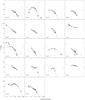 |
Fig. 3 SEDs of the 18 BAL QSOs observed during the m/mm-wavelengths campaign (x-axis: GHz; y-axis: mJy). 235 MHz and 610 MHz flux densities from the GMRT; 250 GHz flux densities from IRAM-30 m; 345 and 850 GHz flux densities from APEX. Measurements at other frequencies are taken from Bruni et al. (2012), or from our polarimetry campaign (see Sect. 3). Triangles are 3σ upper limits. Solid lines are parabolic or linear fits, according to the criteria discussed in Sect. 4.2. |
5.2. Dust emission
Especially with the advent of the Herschel Space Observatory, several works in recent years have constrained the dust emission properties in AGNs and verified the connection with star formation rate. Here we provide a comparison between our results for BAL QSOs in the mm-band and those of other authors.
A study very similar to ours in terms of instrumentation, sensitivity, and setup is the one presented by Omont et al. (2003). They performed 250-GHz observations of 35 optically luminous RQ QSOs (MB< −27.0), with a similar redshift range to ours (1.8<z<2.8), which was performed with the MAMBO bolometer at the same frequency. They found that 26 ± 9% of the sources present an emission at that frequency. Since they reached an rms very similar to our observations (~1 mJy), we can compare our detection rate with this percentage: only 1 out of 17 (~6%) of our sources shows 250-GHz emission that is attributable to dust, a substantially smaller fraction than the one found by these authors.
More recently, Kalfountzou et al. (2014) have published results of the Herschel-ATLAS project regarding FIR properties of RL and RQ QSOs. Using five different bands (100, 160, 250, 350, 500 μm) they fitted the dust emission for both groups. At the mean redshift of our sample (z ~ 2.3), they found a mean flux density for RL QSOs of 23.5 ± 2.1 mJy at 350 μm (corresponding to our 850 GHz observations) and 21.3 ± 2.8 mJy at 500 μm (~600 GHz). These are values below the sensitivity we reached with APEX, but using a simple power law to extract the expected mean flux density at 250 GHz from the previous values, we obtain a value of ~17 mJy that would be detectable with the rms of ~1 mJy we could reach at IRAM-30 m. This could suggest that our sample of RL BAL QSOs is also poorer in dust content than normal RL QSOs, in addition to RQ ones (as seen when comparing with Omont et al. 2003).
In light of these works, our results support the idea of BAL QSOs not being especially dusty objects. In addition, although with modest statistical significance, our work suggests that dust emission in the RL BAL QSO subclass could be weaker than expected. Tombesi et al. (2015) find that fast outflows (~0.25c) from the accretion disk in AGNs can hamper star formation, affecting the interstellar medium. Although at a lower ionisation stage than the ones considered by those authors, BAL-producing outflows can present velocities up to 0.2c, and, in light of these results, could have a similar effect on the SFR of the host galaxy. This needs to be investigated with further observations, which could confirm this on larger samples of RL BAL QSOs.
6. Conclusions
We performed observations in the m band with the GMRT of five RL BAL QSOs that already showed hints of emission in the MHz range and in the mm bands for 17 RL BAL QSOs from our previously studied sample. We aimed at exploring the emission in the low-frequency regime and the grey-body emission from dust, respectively. The conclusions are the following.
All five objects that were observed at low frequencies present emission from extended components, indicating the presence of an old radio emission. In some cases a restarting radio activity can be invoked to explain the double component, MHz- and GHz-peaked, present in their SEDs. This could suggest an intermittent BAL phase, which is associated with periods of radio-restarting activity. This is also supported by the morphology of some objects, both from this work (0849+27) and from Bruni et al. (2013), and by the possibility that ~70% of our RL BAL QSOs sample is in a GPS or CSS+GPS phase, thanks to the data presented here.
Only 1 out of 17 sources (~6%) presents a clear contribution at 250 GHz from the dust grey-body emission. In the other cases, 3σ upper limits have been derived. Comparing our results with the fraction of dust-rich RQ QSOs found by Omont et al. (2003), resulting in a percentage of ~26%, we found that RL BAL QSOs do not present a larger percentage of dust-rich objects than in the RQ QSO population. Also comparing with more recent works from the Herschel-ATLAS collaboration (Kalfountzou et al. 2014), we found a lack of dust emission with respect to mean values for RL QSOs. Since the amount of dust can be connected to star formation and thus to the age of the host galaxy, this result suggests that RL BAL QSOs are not a hosted by particularly young galaxies. That despite radio loudness, these objects present even less dust emission (and consequently a lower star formation rate) than RQ QSOs could suggest that BAL-producing outflows are able to hamper star formation in the host galaxy.
Both the results from observations performed at m and mm wavelengths suggest that BAL QSOs are not commonly young radio objects or objects still expelling their dust cocoon from the central region. They could be radio-restarting objects, which present relativistic outflows in conjunction with some periods of favourable emission or acceleration conditions.
I.e. we adopted an AI defined as 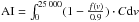 , as in Hall et al. (2002), but with C = 1 only for contiguous troughs ≥1000 km s-1, and nought otherwise.
Acknowledgments
Part of this work was supported by a grant of the Italian Programme for Research of National Interest (PRIN No. 18/2007, PI: K.-H. Mack) The authors acknowledge financial support from the Spanish Ministerio de Ciencia e Innovación under project AYA2008-06311-C02-02. We thank the staff of the GMRT that made these observations possible. GMRT is run by the National Centre for Radio Astrophysics of the Tata Institute of Fundamental Research. This publication is based on data acquired with the Atacama Pathfinder Experiment (APEX). APEX is a collaboration between the Max-Planck-Institut für Radioastronomie, the European Southern Observatory, and the Onsala Space Observatory. This work is partly based on observations carried out with the IRAM-30 m Telescope. IRAM is supported by INSU/CNRS (France), MPG (Germany) and IGN (Spain).
References
- Adelman-McCarthy, J. K., Agüeros, M. A., Allam, S. S., et al. 2007, ApJS, 172, 634 [NASA ADS] [CrossRef] [Google Scholar]
- Allen, J. T., Hewett, P. C., Maddox, N., et al. 2011, MNRAS, 410, 860 [NASA ADS] [CrossRef] [Google Scholar]
- Becker, R. H., White, R. L., Gregg, M. D., et al. 2001, ApJS, 135, 227 [NASA ADS] [CrossRef] [Google Scholar]
- Best, P. N., Kaufmann, G., Heckman, T. M., et al. 2005, MNRAS, 362, 25 [NASA ADS] [CrossRef] [Google Scholar]
- Briggs, F. H., Turnsheck, D. A., & Wolfe, M. 1984, ApJ, 287, 549 [NASA ADS] [CrossRef] [Google Scholar]
- Brocksopp, C., Kaiser, C. R., Schoenmakers, A. P., et al. 2007, MNRAS, 382, 1019 [NASA ADS] [CrossRef] [Google Scholar]
- Bruni, G., Mack, K.-H., Salerno, E., et al., 2012, A&A, 542, A13 [NASA ADS] [CrossRef] [EDP Sciences] [Google Scholar]
- Bruni, G., Dallacasa, D., Mack, K.-H., et al. 2013, A&A, 554, A94 [NASA ADS] [CrossRef] [EDP Sciences] [Google Scholar]
- Bruni, G., González-Serrano, J.-I., Pedani, M., et al. 2014, A&A, 569, A87 [NASA ADS] [CrossRef] [EDP Sciences] [Google Scholar]
- Cao Orjales, J. M., Stevens, J. A., Jarvis, M. J., et al. 2012, MNRAS, 427, 1209 [NASA ADS] [CrossRef] [Google Scholar]
- Capellupo, D. M., Hamann, F., Shields, J. C., et al. 2011, MNRAS, 413, 908 [NASA ADS] [CrossRef] [Google Scholar]
- Capellupo, D. M., Hamann, F., Shields, J. C., et al. 2012, MNRAS, 422, 3249 [NASA ADS] [CrossRef] [Google Scholar]
- Czerny, B., Siemiginowska, A., Janiuk, A., et al. 2009, ApJ, 698, 840 [NASA ADS] [CrossRef] [Google Scholar]
- Dallacasa, D., Stanghellini, C., Centoza, M., et al. 2000, A&A, 363, 887 [NASA ADS] [Google Scholar]
- da Cunha, E., Charlot, S., & Elbaz, D. 2008, MNRAS, 388, 1595 [NASA ADS] [CrossRef] [Google Scholar]
- DiPompeo, M. A., Brotherton, M. S., De Breuck, C., et al. 2011, ApJ, 743, 71 [NASA ADS] [CrossRef] [Google Scholar]
- Dunne, L., Eales, S., Edmunds, M., et al. 2000, MNRAS, 315, 115 [NASA ADS] [CrossRef] [Google Scholar]
- Dunne, L., Gomez, H. L., da Cunha, E., et al. 2011, MNRAS, 417, 1510 [NASA ADS] [CrossRef] [Google Scholar]
- Elvis, M. 2000, ApJ, 545, 63 [NASA ADS] [CrossRef] [Google Scholar]
- Farrah, D., Lacy, M., Priddey, R., et al. 2007, ApJ, 662, 59 [Google Scholar]
- Feruglio, C., Maiolino, R., Piconcelli, E., et al. 2010, A&A, 518, L155 [NASA ADS] [CrossRef] [EDP Sciences] [Google Scholar]
- Filiz Ak, N., Brandt, W. N., Hall, P. B., et al. 2012, ApJ, 757, 114 [NASA ADS] [CrossRef] [Google Scholar]
- Filiz Ak, N., Brandt, W. N., Hall, P. B., et al. 2013, ApJ, 777, 168 [NASA ADS] [CrossRef] [Google Scholar]
- Ganguly, R., & Brotherton, M. S. 2008, ApJ, 672, 102 [NASA ADS] [CrossRef] [Google Scholar]
- Gibson, R. R., Brandt, W. N., Schneider, D. P., et al. 2008, ApJ, 675, 985 [NASA ADS] [CrossRef] [Google Scholar]
- Gibson, R. R., Brandt, W. N., Gallagher, S. C., et al. 2010, ApJ, 713, 220 [NASA ADS] [CrossRef] [Google Scholar]
- Hall, P. B., Anderson, S. F., Strauss, M. A., et al. 2002, ApJS, 141, 267 [NASA ADS] [CrossRef] [Google Scholar]
- Harrison, C. M., Alexander, D. M., Mullaney, G. R., et al. 2014, MNRAS, 441, 3306 [Google Scholar]
- Hayashi, T. J., Doi, A., & Nagai, H. 2013, ApJ, 772, 4 [NASA ADS] [CrossRef] [Google Scholar]
- Hewett, P. C., & Foltz, C. B. 2003, AJ, 125, 1784 [NASA ADS] [CrossRef] [Google Scholar]
- Hughes, D. H., Dunlop, J. S., & Rawlings, S. 1997, MNRAS, 289, 766 [NASA ADS] [CrossRef] [Google Scholar]
- Kalfountzou, E., Stevens, J. A., Jarvis, M. J., et al. 2014, MNRAS, 442, 1181 [NASA ADS] [CrossRef] [Google Scholar]
- Konar, C., Saikia, D. J., Jamrozy, M., et al. 2006, MNRAS, 372, 693 [NASA ADS] [CrossRef] [Google Scholar]
- Konar, C., Hardcastle, M. J., Jamrozy, M., & Croston, J. H. 2013, MNRAS, 430, 2137 [NASA ADS] [CrossRef] [Google Scholar]
- Kunert-Bajraszewska, M., Janiuk, A., Gawrónski, M. P., & Siemiginowska, A. 2010, ApJ, 718, 1345 [NASA ADS] [CrossRef] [Google Scholar]
- Lara, L., Márquez, I., Cotton, W. D., et al. 1999, A&A, 348, 699 [NASA ADS] [Google Scholar]
- Marecki, A., Thomasson, P., Mack, K.-H., et al. 2006, A&A, 448, 479 [NASA ADS] [CrossRef] [EDP Sciences] [Google Scholar]
- Montenegro-Montes, F. M., Mack, K.-H., Vigotti, M., et al. 2008, MNRAS, 388, 1853 [NASA ADS] [CrossRef] [Google Scholar]
- Nandi, S., Roy, R., Saikia, D. J., et al. 2014, ApJ, 789, 16 [NASA ADS] [CrossRef] [Google Scholar]
- O’Dea, C. P. 1998, PASP, 110, 493 [NASA ADS] [CrossRef] [Google Scholar]
- Omont, A., Beelen, A., Bertoldi, F., et al. 2003, A&A, 398, 857 [NASA ADS] [CrossRef] [EDP Sciences] [Google Scholar]
- Orienti, M., & Dallacasa, D. 2008, A&A, 477, 807 [NASA ADS] [CrossRef] [EDP Sciences] [Google Scholar]
- Pounds, K. A., Reeves, J. N., King, A. R., et al. 2003, MNRAS, 345, 705 [NASA ADS] [CrossRef] [Google Scholar]
- Priddey, R. S., Gallagher, S. C., Isaak, K. G., et al. 2007, MNRAS, 374, 867 [NASA ADS] [CrossRef] [Google Scholar]
- Rochais, T. B., DiPompeo, M. A., Myers, A. D., et al. 2014, MNRAS, 444, 2498 [NASA ADS] [CrossRef] [Google Scholar]
- Saikia, D. J., & Jamrozy, M. 2009, BASI, 37, 63 [Google Scholar]
- Sanders, D. M. 2002, ASP Conf. Ser., 284 [Google Scholar]
- Schneider, D. P., Hall, P. B., Richards, G. T., et al. 2007, AJ, 134, 102 [NASA ADS] [CrossRef] [Google Scholar]
- Schoenmakers, A. P., de Bruyn, A. G., Rüttgering, H. J. A., et al. 2000, MNRAS, 315, 371 [NASA ADS] [CrossRef] [Google Scholar]
- Shabala, S. S., Ash, S., Alexander, P., et al. 2008, MNRAS, 388, 625 [NASA ADS] [CrossRef] [Google Scholar]
- Siringo, G., Kreysa, E., Kovács, A., et al. 2009, A&A, 497, 945 [NASA ADS] [CrossRef] [EDP Sciences] [Google Scholar]
- Siringo, G., Kreysa, E., De Breuck, C., et al. 2010, The Messenger, 139, 20 [NASA ADS] [Google Scholar]
- Stanghellini, C., Baum, S. A., O’Dea, C. P., et al. 1990, A&A, 233, 379 [NASA ADS] [Google Scholar]
- Stanghellini, C., O’Dea, C. P., Dallacasa, D., et al. 2005, A&A, 443, 891 [NASA ADS] [CrossRef] [EDP Sciences] [Google Scholar]
- Sturm, E., González-Alfonso, E., & Veilleux, S. 2011, ApJ, 733, L16 [NASA ADS] [CrossRef] [Google Scholar]
- Stocke, J. T., Morris, S. L., Weymann, R. J., et al. 1992, ApJ, 396, 487 [NASA ADS] [CrossRef] [Google Scholar]
- Tombesi, F., Tazaki, F., Mushotzky, R. F., et al. 2014, MNRAS, 443, 2154 [NASA ADS] [CrossRef] [Google Scholar]
- Tombesi, F., Meléndez, M., Veilleux, S., et al. 2015, Nature, 519, 436 [Google Scholar]
- Vivek, M., Srianand, R., Petitjean, P., et al. 2012, MNRAS, 423, 2879 [NASA ADS] [CrossRef] [Google Scholar]
- Willott, C. J., Rawlings, S., & Grimes, J. A. 2003, ApJ, 598, 909 [NASA ADS] [CrossRef] [Google Scholar]
- Wang, P., Li, Z.-Y., Abel, T., et al. 2010, ApJ, 709, 27 [NASA ADS] [CrossRef] [Google Scholar]
- Wu, Q. 2009, ApJ, 701, L95 [NASA ADS] [CrossRef] [Google Scholar]
- Zahid, H. J., Kashino, D., Silverman, J. D., et al. 2014, ApJ, 792, 75 [NASA ADS] [CrossRef] [Google Scholar]
All Tables
Revised flux densities (top lines) and measurements from our polarimetry campaign (bottom lines).
Results for the 17 BAL QSOs observed in the mm band: 250 GHz flux densities from IRAM-30 m, 345, and 850 GHz from APEX.
All Figures
|
Fig. 1 Maps of BAL QSO 0849+27 from the FIRST survey (left panel – 1.4 GHz, beam 5.40 × 5.40 arcsec), our EVLA observations (central panel – 4.86 GHz, beam 1.95 × 1.25 arcsec), and our VLBA observations ((right panel – 5 GHz, beam 2.99 × 1.15 mas). Contours are multiples of 3σ, according to the label. Dashed contours are negative. The synthesised beam size is shown in the lower left corner of each map. The scale of the right panel is in mas. |
| In the text | |
|
Fig. 2 Maps of 5 BAL QSOs observed with the GMRT at 235 and 610 MHz. Contours are multiples of 3σ, according to the label. Dashed contours are negative. The synthesised beam size is shown in the lower left corner of each map. |
| In the text | |
|
Fig. 3 SEDs of the 18 BAL QSOs observed during the m/mm-wavelengths campaign (x-axis: GHz; y-axis: mJy). 235 MHz and 610 MHz flux densities from the GMRT; 250 GHz flux densities from IRAM-30 m; 345 and 850 GHz flux densities from APEX. Measurements at other frequencies are taken from Bruni et al. (2012), or from our polarimetry campaign (see Sect. 3). Triangles are 3σ upper limits. Solid lines are parabolic or linear fits, according to the criteria discussed in Sect. 4.2. |
| In the text | |
Current usage metrics show cumulative count of Article Views (full-text article views including HTML views, PDF and ePub downloads, according to the available data) and Abstracts Views on Vision4Press platform.
Data correspond to usage on the plateform after 2015. The current usage metrics is available 48-96 hours after online publication and is updated daily on week days.
Initial download of the metrics may take a while.