Erratum for: A&A 557, A93 (2012), DOI: 10.1051/0004-6361/201220779

1. Background

In Figueira et al. (2013) we proposed a new line profile variation indicator, V_asy. For a given spectral line, this indicator evaluates the asymmetry in the radial velocity (RV) information content. By evaluating this asymmetry and associating the quantity to an RV variation, it is possible to identify whether the variation stems from a deformation of the line profile or from a bona fide RV shift. In Figueira et al. (2013) we defined that ${\mathit{V}}_{\mathrm{asy}}\mathrm{=}\frac{{\sum }_{\mathrm{flux}}\mathrm{\left(}{\mathit{W}}_{\mathit{i}}\mathrm{\right(}\mathrm{red}\mathrm{)}\mathrm{-}{\mathit{W}}_{\mathit{i}}\mathrm{(}\mathrm{blue}\mathrm{\left)}\mathrm{\right)}\mathrm{\times }\overline{{\mathit{W}}_{\mathit{i}}}}{{\sum }_{\mathrm{flux}}\overline{{\mathit{W}}_{\mathit{i}}}}$(1)in which W_i are the weights of the point calculated at the flux level i, as defined in Eq. (8) of Bouchy et al. (2001), where ${\mathit{W}}_{\mathit{i}}\mathrm{=}\frac{{\mathit{\lambda }}^{\mathrm{2}}\mathrm{\left(}\mathit{i}\mathrm{\right)}\mathrm{\left(}\mathit{\partial }{\mathit{A}}_{\mathrm{0}}\mathrm{\right(}\mathit{i}\mathrm{)}\mathit{/}\mathit{\partial \lambda }\mathrm{(}\mathit{i}\mathrm{)}{\mathrm{)}}^{\mathrm{2}}}{{\mathit{A}}_{\mathrm{0}}\mathrm{\left(}\mathit{i}\mathrm{\right)}\mathrm{+}{\mathit{\sigma }}_{\mathrm{D}}^{\mathrm{2}}}$(2)with λ(i) and A₀(i) representing the wavelength and flux of the spectra, respectively, and ${\mathit{\sigma }}_{\mathrm{D}}^{\mathrm{2}}$ the detector readout noise. Since we are working in the velocity space, the wavelength is a velocity. This is standard procedure and has been applied extensively to the cross-correlation function (CCF). Moreover, we are working in a very high signal-to-noise domain as such, ${\mathit{A}}_{\mathrm{0}}\mathrm{\left(}\mathit{i}\mathrm{\right)}\mathrm{+}{\mathit{\sigma }}_{\mathrm{D}}^{\mathrm{2}}\mathrm{\approx }{\mathit{A}}_{\mathrm{0}}\mathrm{\left(}\mathit{i}\mathrm{\right)}$. We can then rewrite the previous equation in the form of 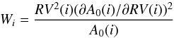${\mathit{W}}_{\mathit{i}}\mathrm{=}\frac{\mathit{R}{\mathit{V}}^{\mathrm{2}}\mathrm{\left(}\mathit{i}\mathrm{\right)}\mathrm{\left(}\mathit{\partial }{\mathit{A}}_{\mathrm{0}}\mathrm{\right(}\mathit{i}\mathrm{)}\mathit{/}\mathit{\partial RV}\mathrm{(}\mathit{i}\mathrm{)}{\mathrm{)}}^{\mathrm{2}}}{{\mathit{A}}_{\mathrm{0}}\mathrm{\left(}\mathit{i}\mathrm{\right)}}$(3)in which RV(i) is the RV value of each pixel (i.e. x-axis) of the CCF. For every flux level i, we consider three quantities: the blue wing information, W_i(blue); the red wing information, W_i(red); and the average between the two, $\overline{{\mathit{W}}_{\mathit{i}}}\mathrm{=}\mathrm{\left(}{\mathit{W}}_{\mathit{i}}\mathrm{\right(}\mathrm{blue}\mathrm{)}\mathrm{+}{\mathit{W}}_{\mathit{i}}\mathrm{(}\mathrm{red}\mathrm{\left)}\mathrm{\right)}\mathit{/}\mathrm{2}$, as representative of the weight of the information content at this flux level for an undeformed line.

2. Correction

While the principle of the V_asy is sound, Eq. (8) of Bouchy et al. (2001) was developed for a spectrum defined in the wavelength domain and cannot be directly applied to the velocity space of the CCF. As a consequence, to translate the principle to velocity space we have to calculate the relative weight of each pixel by directly applying their Eq. (5); this allows us to calculate the weight of a pixel as the inverse of the square of its rms velocity. By applying a Taylor expansion to the error on the radial velocity as a function of the error on the CCF, and considering only the first term, we have ${\mathit{W}}_{\mathit{i}}\mathrm{=}\frac{{\mathit{c}}^{\mathrm{2}}}{{{\mathit{\sigma }}_{\mathrm{RV}}\mathrm{\left(}\mathit{i}\mathrm{\right)}}^{\mathrm{2}}}\mathrm{=}{\mathit{c}}^{\mathrm{2}}\frac{\mathit{\partial }\hspace{0.17em}\mathrm{\left(}\mathrm{CCF}\mathrm{\right(}\mathit{i}\mathrm{)}\mathit{/}\mathit{\partial RV}\mathrm{(}\mathit{i}\mathrm{)}{\mathrm{)}}^{\mathrm{2}}}{{{\mathit{\sigma }}_{\mathrm{CCF}}\mathrm{\left(}\mathit{i}\mathrm{\right)}}^{\mathrm{2}}}$(4)in which σ_CCF(i) represents the error on the RV as induced by the flux measurement in the pixel i, and c is the speed of light. This is assumed to be photon-noise dominated, and can be calculated by recovering the flux contribution to each of the pixels considered in the CCF. As a first approximation it is possible to estimate the error as calculated for the whole spectrum by considering that ${\mathit{\sigma }}_{\mathrm{spec}}\mathrm{=}\sqrt{{\mathrm{\Sigma }}_{\mathit{i}}{\mathit{\sigma }}_{\mathit{i}}^{\mathrm{2}}}$; for a finer estimate the error can be considered to be proportional to the flux in the photon-dominated regime (as is the case), and the error per pixel can be deduced from an estimate on the contrast of the CCF.

2.1. Information content in the CCF

Central to the previous discussion is the issue of the information content of the pseudo-pixel generated by the CCF. While in a real spectra the pixel flux counts correspond to photons, and thus each pixel contains independent flux information that translates into RV information, the same is not true for the CCF. The CCF is calculated using a smaller step in RV than the pixel size in order to avoid information loss when moving across adjacent pixels (see e.g. Baranne et al. 1996; Pepe et al. 2002) and to provide a smoother profile that makes the analysis of BIS easier (Queloz et al. 2001). However, one has to bear in mind that adjacent pixels in the CCF function share photons from the original spectra, and as a consequence flux counts and information content are correlated. The ratio of repeated or correlated pixel count versus spectral pixel count is given by the ratio α_corr = (size of pixel in RV)/(step used in CCF calculation). This means that in order to evaluate the content of information in a CCF we have to consider 1 in every α_corr pixels, or, to put it differentely, we have to evaluate it over a grid in which pixels are spaced by (on average) α_corr. So in order to apply Eq. (4) to the CCF, we have to consider only 1 pixel every α_corr.

2.2. Information content as projected on the flux level

From the previous digression we know how to calculate the information content by applying Eq. (4) to the CCF. A final point remains, which is particular to V_asy. In order to calculate the information content of a spectrum we can simply consider a grid in which the CCF pixels are separated by α_corr; instead, the calculation of V_asy from Eq. (1) is done at constant flux levels. This can be done at any flux level grid that covers the line profile, and in Figueira et al. (2013) we chose to do it over an equidistant interpolated flux grid as inherited from (Queloz et al. 2001).

From the previous section, we conclude that the flux grid chosen has to be such that it projects onto a grid of pixels separated (on average) by α_corr. This can be done by knowing the shape of the function CCF(RV), or CCF(i) to retain the previous notation.

3. Application and results

We applied the modifications described to the implementation of V_asy; for the oversampling factor we considered a value of 3.28, calculated for the HARPS spectrograph, and for the

noise we considered the value stored in the DRS FITS keyword DRS CCF NOISE for σ_spec. For the case of HD 224789, we got a Pearson’s correlation coefficient of 0.45, with a lower absolute value than the one obtained for the BIS, of –0.82. The application to other stars and theoretical cases derived from SOAP (Boisse et al. 2012; Oshagh et al. 2013) also yield lower correlation coefficients than presented with the previous formula. Given this lower efficiency on demonstrated correlations and the possible introduction of spurious correlations as mentioned in Santerne et al. (2015), we advise against the usage of V_asy as a line profile indicator. We note that the online version of V_asy (described in Santos et al. 2014) already reflects these modifications. We refer the interested reader to the recent work of Lanza et al. (2015)¹ for an improved version of V_asy.

Acknowledgments

This work was supported by Fundação para a Ciência e a Tecnologia (FCT) through the research grant UID/FIS/04434/2013. P.F. and N.C.S. acknowledge support by Fundação para a Ciência e a Tecnologia (FCT) through Investigador FCT contracts of reference IF/01037/2013 and IF/00169/2012, respectively, and POPH/FSE (EC) by FEDER funding through the program “Programa Operacional de Factores de Competitividade – COMPETE”. P.F. further acknowledges support from Fundação para a Ciência e a Tecnologia (FCT) in the form of an exploratory project of reference IF/01037/2013CP1191/CT0001. P.F. warmly thanks Heather Cegla and Chris Watson for pointing out the limitations of Vasy’s implementation, and Alexandre Santerne for interesting discussions on the subject.

References

© ESO, 2015

References

- Baranne, A., Queloz, D., Mayor, M., et al. 1996, A&AS, 119, 373 [NASA ADS] [CrossRef] [EDP Sciences] [Google Scholar]
- Boisse, I., Bonfils, X., & Santos, N. C. 2012, A&A, 545, A109 [NASA ADS] [CrossRef] [EDP Sciences] [Google Scholar]
- Bouchy, F., Pepe, F., & Queloz, D. 2001, A&A, 374, 733 [NASA ADS] [CrossRef] [EDP Sciences] [Google Scholar]
- Figueira, P., Santos, N. C., Pepe, F., Lovis, C., & Nardetto, N. 2013, A&A, 557, A93 [NASA ADS] [CrossRef] [EDP Sciences] [Google Scholar]
- Oshagh, M., Boisse, I., Boué, G., et al. 2013, A&A, 549, A35 [NASA ADS] [CrossRef] [EDP Sciences] [Google Scholar]
- Pepe, F., Mayor, M., Galland, F., et al. 2002, A&A, 388, 632 [NASA ADS] [CrossRef] [EDP Sciences] [Google Scholar]
- Queloz, D., Henry, G. W., Sivan, J. P., et al. 2001, A&A, 379, 279 [NASA ADS] [CrossRef] [EDP Sciences] [Google Scholar]
- Santerne, A., Díaz, R. F., Almenara, J.-M., et al. 2015, MNRAS, 451, 2337 [NASA ADS] [CrossRef] [Google Scholar]
- Santos, N. C., Mortier, A., Faria, J. P., et al. 2014, A&A, 566, A35 [NASA ADS] [CrossRef] [EDP Sciences] [Google Scholar]
© ESO, 2015
Current usage metrics show cumulative count of Article Views (full-text article views including HTML views, PDF and ePub downloads, according to the available data) and Abstracts Views on Vision4Press platform.
Data correspond to usage on the plateform after 2015. The current usage metrics is available 48-96 hours after online publication and is updated daily on week days.
Initial download of the metrics may take a while.