© ESO, 2015

1. Introduction

The UV to optical color ratio of the total AGN, measured in magnitude units, becomes bluer as the AGN brightens (e.g. Meusinger et al. 2011). Some studies attribute this change in color to the spectral hardening of the variable component (Giveon et al. 1999; Wilhite et al. 2005; Wamsteker et al. 1990; Webb & Malkan 2000). However, there is ample evidence to suggest that the color of the variable component stays constant and that the corresponding flux variation gradient is offset from the origin of the flux-flux diagram (Choloniewski 1981; Winkler et al. 1992; Winkler 1997; Paltani & Walter 1996; Sakata et al. 2010). In this case, the “bluer when brighter” total observed fluxes, which are measured in a finite aperture, are explained by the superimposition of a constant red host galaxy (including non-varying emission lines) and a varying blue AGN. Even if the measured host contribution is small, compared to the required offset of the flux variation gradient (FVG), there is no significant curvature seen in the flux-flux diagrams (Sakata et al. 2011).

The constancy of the optical colors of the variable component is physically plausible if the variable emission has a hot thermal origin, as expected for an accretion disk (AD). In this case, fluxes in the optical range lie on the Rayleigh-Jeans tail, and they scale almost linearly with temperature.

Recently, Sun et al. (2014) report time-dependent g/r color variability of the SDSS Stripe 82 quasar sample. A blue color at variations inside <30 days (with smaller amplitudes) gradually changes to redder colors on larger timescales >1000 days (and larger amplitudes). Furthermore, Sun et al. (2014) claim that the FVG method lacks rigor and is, therefore, not valid. Consequently, one also expects to find similar behavior for Seyfert galaxies, the less luminous siblings of quasars.

Using data from 2009–2010, Pozo Nuñez et al. (2012) performed B-, V-band monitoring of the Seyfert 1 Galaxy 3C 120 including dense daily observations over a period of five months. Here we report new B-, V-band results from a six-month monitoring project in 2014 and 2015. The total brightening (by about 1.4 mag) and the dense time-sampling of observations allow us to check whether or not brightness and time-dependent color variations are present.

2. Observations and data reduction

The new photometric data at Johnson B and V was observed between 27 August 2014 and 3 March 2015 at the Universitätssternwarte Bochum, near Cerro Armazones. We combined the RoBoTT telescope data (Pozo Nuñez et al. 2012) with new data from the BEST II (Kabath et al. 2009).

All data has been corrected for the latest revision of galactic foreground extinction¹ by Schlafly & Finkbeiner (2011) and the corresponding lightcurves are displayed in Figs.1 and 2.

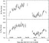	Fig. 1 Lightcurves in the 2009–2010 epoch obtained with the RoBoTT telescope. All fluxes are corrected for galactic foreground extinction.
Open with DEXTER

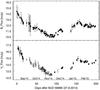	Fig. 2 Combined lightcurves in the 2014–2015 epoch, obtained with two different telescopes. Filled circles correspond to BEST II, while open triangles represent the RoBoTT observations. All fluxes are corrected for galactic foreground extinction.
Open with DEXTER

3. Results

3.1. Flux-flux diagrams

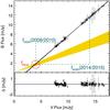Fig. 3 B versus V flux variations of 3C 120 in the aperture. Each measurement is drawn as a thin cross in which the line length corresponds to the photometric uncertainties in the respective filters. The yellow filled area is the assumed host color ΓBV,Host, drawn to cover B = (1.70 ± 0.27) mJy and V = (4.01 ± 0.62) mJy host fluxes, as determined by Sakata et al. (2010) in an aperture. Our host flux estimate is the datapoint in the red circle. All data from 2009 until 2015 was used to determine the AGN slope. The black continuous line covers the upper and lower standard deviations in the AGN slope, given by the OLS bisector fit.

Open with DEXTER

Total B- versus V-band fluxes for the two epochs are shown in Fig. 3, with one that had low luminosity in 2009–2010 and one that had high luminosity in 2014–2015. Between the two epochs, the AGN luminosity increased by a magnitude of about 1.4 in both filters. The slope of AGN variability is well matched by a linear relation with Γ_BV = 0.979 ± 0.005.

We consider the host colors of 3C 120 by Sakata et al. (2010) in a aperture, corrected for galactic foreground extinction (Schlafly & Finkbeiner 2011). Assuming that these will be similar when looked at in our aperture, this allows us to compute our own host fluxes by measuring the center of gravity of the area that is encased by the cone of AGN slope Γ_BV-fitting uncertainties and Sakata’s host color Γ_BV,Host (inside the red circle of Fig. 3). The results for the B- and V-band host fluxes (Table 1) agree well with the values of Sakata. We also fit the slopes of the individual epochs of 2009–2010 and 2014–2014 separately. For both epochs the slope is slightly flatter than the combined one, but they agree within the errors.

The offset of the combined slope (2009−2015) to the individual epoch slopes could imply that the short-term variability is redder than the long-term one. A more likely physical explanation, however, is based on the systematically different instrumental point spread functions (PSF). The PSF of the RoBoTT is slightly larger than that of the BEST II. The host also has a different spatial flux distribution at B and V. This leads to a larger host galaxy contribution in the 2009−2010 lightcurves, and the host galaxy contribution is larger in V than in B. In the net effect, compared to the 2014−2015 data, the 2009−2010 data appear slightly shifted in the FVG diagram toward the right, resulting in a marginally steeper overall Γ_BV. We believe that these negligible effects do not alter the basic results and conclusions on the stability of the FVG method because for all three data sets (2009−2010, 2014−2015, and 2009−2015) the host galaxy contribution is in excellent agreement within the errors. In B-band we measure a minimum f_B,AGN = 3.59 mJy and a maximum of f_B,AGN = 12.69 mJy. Correspondingly, the increase in V ranges from a minimum of f_V,AGN = 3.57 mJy to a maximum of f_V,AGN = 12.76 mJy.

3.2. Search for timescale-dependent AGN colors

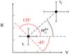Fig. 4 Scheme of the color slope in the B- to V-band flux plane between two measurements ti and tj with photometric uncertainties. If Θ falls below −45° or above 135° we add or subtract 180° respectively. Restricting ourselves to the half circle, marked by the red arcs, ensures proper averaging of for low values of τ, where photometric uncertainties dominate the slopes. A restriction to the full circle, or −90° to 90°, would bias the slope towards 0° if the photometric errors are large compared to the true change of flux.

Open with DEXTER

The aim of this section is to investigate potential, timescale-dependent variability that has recently been observed by Sun et al. (2014) in a sample of Stripe 82 SDSS quasars. The ensemble color variability of their quasars was not constant for all observed redshifts, showing rather blue slopes on short timescales of <30 days that turn to redder slopes on longer timescales.

Here we improve their approach in some aspects. Instead of using magnitudes, we make use of fluxes f_ν directly. As pointed out by Kokubo et al. (2014) and references therein, fitting a straight line in magnitude–magnitude space (e.g. Sun et al. 2014) relies heavily on the contamination of the baseline flux by host galaxies and emission lines.

The color of an arbitrary flux variation in B- and V-band in the time interval τ = | t_j − t_i | is computed using Eq. (1). The geometry is explained in Fig. 4. 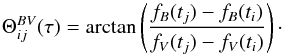(1)Like Sun et al. (2014), we restrict ourselves to the range of slopes . The slopes on the other half circle represent flux decreases and are rotated by 180° to their equivalent slopes for a flux increase. The offset of 45° is chosen to equally weigh cases of both bluer (i) when brighter (); and (ii) redder, when brighter (), slopes in the averaging process. The angle of 45° represents no color change.

Our photometric measurements in all observed epochs offer for many combinations of t_i and t_j, with the lowest sampling interval of τ = 1 day. It is useful to average all inside bins with this size. The average of these bins is described by (2)The results of this approach for the B- and V-band fluxes are shown in Fig. 5, together with the structure function S(τ), as defined by Eq. (3). The latter is an indicator of the strength of the variability on a specific time scale τ. The black solid lines enclose the average photometric uncertainty of each τ bin. (3)Analyzing photometric fluxes with large uncertainties σ_i,σ_j, compared to the difference in fluxes with , can cause a bias on Θ_ij. We assume a case of flux that is constant except for noise that is described by different photometric uncertainties for B- and V-band with σ_fB ≫ σ_fV. Then, referring to the sketch in Fig. 4, we have Δf_B ≫ Δf_v for samples of measurements drawn from these distributions. As a result, we obtain .

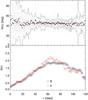Fig. 5 Top: small dots represent between all possible permutations of measurements i,j with τ = | tj − ti |. Larger dots mark the averages inside a bin of one day with their uncertainty plotted as a continuous black line. The red straight line at 44.4° corresponds to the linear fit of all data ΓBV = 0.979. Bottom: the structure function S of the variability; black boxes for B-band and red diamonds for V-band.

Open with DEXTER

The structure function S(τ) for the short timescales in Fig. 5 shows that for τ< 20 days the variations are still on the order of typical photometric errors. As a consequence, the distribution of is very broad in this region. The shape of the structure function is very similar for both bands with a slightly larger variation in amplitudes around 60 days for the V-band. For comparison purposes, we plot the previous linear fit result of Γ_BV = 0.979 as solid red line. In this early epoch, the majority of slopes is about 3° higher than the linear approximation but with only low significance and large scatter. From 20 to 90 days, the scatter decreases and the average cannot be distinguished from the linear fit. A potential contribution of ~5% Hβ at 25 days (Pozo Nuñez et al. 2012) may introduce additional flux to the V-band and shifts the slope downward in this region. However, there is no significant trace of this effect. After 90 days, the number of data points in the τ bins decreases naturally, causing larger scatter and a minimally lower average slope of 42°. In summary, the plot reveals no clear difference in on timescales τ within a single observation epoch of 3C 120.

	Fig. 6 Same as Fig. 5, here for the high values of τ between the epochs of 2009–2010 and 2014–2015.
Open with DEXTER

In Fig. 6, we restrict the plot to 1640 <τ< 1960, so that all have one data point in our early epoch of 2009–2010 and one in the late epoch of 2014–2015. In total, all angles are consistent with our linear fit result, taking the photometric uncertainties into consideration. Within the errors, there appears a positive slope from 44° to 45° for the considered range of τ. This is, however, consistent with a potential host flux offset between the two epochs that originates from different PSFs as explained in Sect. 3.1.

4. Discussion and conclusions

Our results show a highly linear evolution of B versus V fluxes for 3C 120 on all timescales – from days to several years. Additionally, the color is highly constant, despite the AGN undergoing a strong increase of 1.4 mag in flux over a duration of five years.

Calculating their time dependent colors θ(τ) in magnitude-magnitude space, Sun et al. (2014) report a significant change of color for g- and r-band data of a large SDSS quasar sample. The colors change from short timescale (small amplitude) blue colors to long timescale (large amplitude) red colors. Considering a total observed flux f(t) = f_Host + f_AGN(t), composed of constant host galaxy component and variable AGN, the difference in magnitude space is 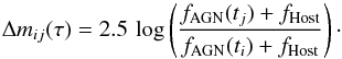(4)This means that a constant host causes a reduction in the observed magnitude difference. Because the host galaxy SED is red, compared to that of the AGN, the magnitude difference will be reduced more for the red Δm_r(τ) compared to the blue Δm_g(τ) and therefore θ(τ) = arctan(Δm_r(τ) / Δm_g(τ)) turns to artificially blue colors. Since the structure function of the SDSS quasars rises towards long timescales (Sun et al. 2014), we simultaneously observe large amplitudes of flux variations. Because the host galaxy contribution is reduced in such cases, θ(τ) will be of a redder color. In our flux-flux approach, however, this issue is completely avoided. Therefore, we suggest that the luminosity and time-dependent color variability observed by Sun et al. is an artifact of data analysis in magnitudes instead of fluxes.

The intrinsic brightness change of any astronomical object may be caused by a change in the area and/or the temperature T

of the emitting surface. While an increase in area would simply cause a constant color, the temperature change always has a degree of curvature. Only in the Rayleigh-Jeans approximation is the flux again proportional to the temperature T. Using the blue side λ of the Johnson B-band in hc<λk_BT, the temperature T must be higher than 36 000 K, because it is at the lower end of typical effective AD temperatures. The existence of a linear relationship between two (optical) fluxes shows that the variable component is hot enough to be approximated by Rayleigh Jeans.

Another mechanism for a brightness change is variable extinction. In this case, the extinction law influences the color of the varying component, with the bluer band usually more affected than the red band. As a result, extinction can provide a different color slope than a temperature fluctuation in the AD. However, extinction variations resulting from dust clouds that move into the line of sight are random events and should occur with diverse amplitude and timescales. Because they are independent of the variations in the AD with different its color, non-linear behavior of the total fluxes should then be observed in individual objects. Averaging a large sample of AGN flux variations, such random disturbances of the slope in the flux-flux diagrams will be washed out.

Our results are consistent with variations that stem from temperature changes in the AD, where the B- and V-bands are placed in the Rayleigh-Jeans tail of the thermal emission. There is no evidence for a short timescale, bluer color variation that may be caused by variable extinction in the line of sight.

In summary, our finding makes a good case for the use of the rest-frame optical FVG method on different timescales of low luminosity AGN. To further confirm this result, more longterm observations of varying Seyferts (and also quasars) with high photometric precision and dense (daily) temporal sampling will be required.

Acknowledgments

This research made use of the NASA/IPAC Extragalactic Database (NED) which is operated by the Jet Propulsion Laboratory, California Institute of Technology, under contract with the National Aeronautics and Space Administration (NASA). This publication is supported as a project of the Nordrhein-Westfälische Akademie der Wissenschaften und der Künste, in the framework of the academy program of the Federal Republic of Germany and the state of Nordrhein-Westfalen. This work is supported by the DFG Program (HA 3555/12-1). The observations on Cerro Armazones benefited from the support of guardians, Hector Labra, Gerardo Pino, Roberto Munoz, and Francisco Arraya. We thank the referee, Ian Glass, for his helpful comments and careful review of the manuscript.

References

Online material

Appendix A: Measured fluxes

All Tables

All Figures

	Fig. 1 Lightcurves in the 2009–2010 epoch obtained with the RoBoTT telescope. All fluxes are corrected for galactic foreground extinction.
Open with DEXTER
In the text

	Fig. 2 Combined lightcurves in the 2014–2015 epoch, obtained with two different telescopes. Filled circles correspond to BEST II, while open triangles represent the RoBoTT observations. All fluxes are corrected for galactic foreground extinction.
Open with DEXTER
In the text

	Fig. 3 B versus V flux variations of 3C 120 in the aperture. Each measurement is drawn as a thin cross in which the line length corresponds to the photometric uncertainties in the respective filters. The yellow filled area is the assumed host color ΓBV,Host, drawn to cover B = (1.70 ± 0.27) mJy and V = (4.01 ± 0.62) mJy host fluxes, as determined by Sakata et al. (2010) in an aperture. Our host flux estimate is the datapoint in the red circle. All data from 2009 until 2015 was used to determine the AGN slope. The black continuous line covers the upper and lower standard deviations in the AGN slope, given by the OLS bisector fit.
Open with DEXTER
In the text

	Fig. 4 Scheme of the color slope in the B- to V-band flux plane between two measurements ti and tj with photometric uncertainties. If Θ falls below −45° or above 135° we add or subtract 180° respectively. Restricting ourselves to the half circle, marked by the red arcs, ensures proper averaging of for low values of τ, where photometric uncertainties dominate the slopes. A restriction to the full circle, or −90° to 90°, would bias the slope towards 0° if the photometric errors are large compared to the true change of flux.
Open with DEXTER
In the text

	Fig. 5 Top: small dots represent between all possible permutations of measurements i,j with τ = | tj − ti |. Larger dots mark the averages inside a bin of one day with their uncertainty plotted as a continuous black line. The red straight line at 44.4° corresponds to the linear fit of all data ΓBV = 0.979. Bottom: the structure function S of the variability; black boxes for B-band and red diamonds for V-band.
Open with DEXTER
In the text

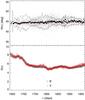	Fig. 6 Same as Fig. 5, here for the high values of τ between the epochs of 2009–2010 and 2014–2015.
Open with DEXTER
In the text

References

- Choloniewski, J. 1981, Acta Astron., 31, 293 [NASA ADS] [Google Scholar]
- Giveon, U., Maoz, D., Kaspi, S., Netzer, H., & Smith, P. S. 1999, MNRAS, 306, 637 [NASA ADS] [CrossRef] [Google Scholar]
- Kabath, P., Erikson, A., Rauer, H., et al. 2009, A&A, 506, 569 [NASA ADS] [CrossRef] [EDP Sciences] [Google Scholar]
- Kokubo, M., Morokuma, T., Minezaki, T., et al. 2014, ApJ, 783, 46 [NASA ADS] [CrossRef] [Google Scholar]
- Meusinger, H., Hinze, A., & de Hoon, A. 2011, A&A, 525, A37 [NASA ADS] [CrossRef] [EDP Sciences] [Google Scholar]
- Paltani, S., & Walter, R. 1996, A&A, 312, 55 [NASA ADS] [Google Scholar]
- Pozo Nuñez, F., Ramolla, M., Westhues, C., et al. 2012, A&A, 545, A84 [NASA ADS] [CrossRef] [EDP Sciences] [Google Scholar]
- Sakata, Y., Minezaki, T., Yoshii, Y., et al. 2010, ApJ, 711, 461 [NASA ADS] [CrossRef] [Google Scholar]
- Sakata, Y., Morokuma, T., Minezaki, T., et al. 2011, ApJ, 731, 50 [NASA ADS] [CrossRef] [Google Scholar]
- Schlafly, E. F., & Finkbeiner, D. P. 2011, ApJ, 737, 103 [NASA ADS] [CrossRef] [Google Scholar]
- Sun, Y.-H., Wang, J.-X., Chen, X.-Y., & Zheng, Z.-Y. 2014, ApJ, 792, 54 [NASA ADS] [CrossRef] [Google Scholar]
- Wamsteker, W., Rodriguez-Pascual, P., Wills, B. J., et al. 1990, ApJ, 354, 446 [NASA ADS] [CrossRef] [Google Scholar]
- Webb, W., & Malkan, M. 2000, ApJ, 540, 652 [NASA ADS] [CrossRef] [Google Scholar]
- Wilhite, B. C., Van den Berk, D. E., Kron, R. G., et al. 2005, ApJ, 633, 638 [NASA ADS] [CrossRef] [Google Scholar]
- Winkler, H. 1997, MNRAS, 292, 273 [NASA ADS] [CrossRef] [Google Scholar]
- Winkler, H., Glass, I. S., van Wyk, F., et al. 1992, MNRAS, 257, 659 [NASA ADS] [Google Scholar]