| Issue |
A&A
Volume 581, September 2015
|
|
|---|---|---|
| Article Number | A129 | |
| Number of page(s) | 18 | |
| Section | Numerical methods and codes | |
| DOI | https://doi.org/10.1051/0004-6361/201526513 | |
| Published online | 22 September 2015 | |
Grid search in stellar parameters: a software for spectrum analysis of single stars and binary systems⋆
Instituut voor Sterrenkunde, KU Leuven, Celestijnenlaan 200D, 3001
Leuven, Belgium
e-mail: This email address is being protected from spambots. You need JavaScript enabled to view it.
Received: 11 May 2015
Accepted: 9 July 2015
Abstract
Context. The currently operating space missions, as well as those that will be launched in the near future, will deliver high-quality data for millions of stellar objects. Since the majority of stellar astrophysical applications still (at least partly) rely on spectroscopic data, an efficient tool for the analysis of medium- to high-resolution spectroscopy is needed.
Aims. We aim at developing an efficient software package for the analysis of medium- to high-resolution spectroscopy of single stars and those in binary systems. The major requirements are that the code should have a high performance, represent the state-of-the-art analysis tool, and provide accurate determinations of atmospheric parameters and chemical compositions for different types of stars.
Methods. We use the method of atmosphere models and spectrum synthesis, which is one of the most commonly used approaches for the analysis of stellar spectra. Our Grid Search in Stellar Parameters (gssp) code makes use of the Message Passing Interface (OpenMPI) implementation, which makes it possible to run in parallel mode. The method is first tested on the simulated data and is then applied to the spectra of real stellar objects.
Results. The majority of test runs on the simulated data were successful in that we were able to recover the initially assumed sets of atmospheric parameters. We experimentally find the limits in signal-to-noise ratios of the input spectra, below which the final set of parameters is significantly affected by the noise. Application of the gssp package to the spectra of three Kepler stars, KIC 11285625, KIC 6352430, and KIC 4931738, was also largely successful. We found an overall agreement of the final sets of the fundamental parameters with the original studies. For KIC 6352430, we found that dependence of the light dilution factor on wavelength cannot be ignored, as it has a significant impact on the determination of the atmospheric parameters of this binary system.
Conclusions. The gssp software package is a compilation of three individual program modules suitable for spectrum analysis of single stars and individual binary components. The code is highly effective and can be used for spectrum analysis of large samples of stars.
Key words: methods: data analysis / stars: variables: general / stars: fundamental parameters / stars: general / binaries: spectroscopic
The gssp software package can be downloaded from https://fys.kuleuven.be/ster/meetings/binary-2015/gssp-software-package
Postdoctoral Fellow of the Fund for Scientific Research (FWO), Flanders, Belgium.
© ESO, 2015
1. Introduction
Nowadays, spectrum analysis is the main source of precise atmospheric parameters and chemical compositions of stars. The problem of chemical composition determination in different classes of stars is directly linked to the problems of production and evolution of chemical elements, stellar and galactic evolution, etc. Interpretation of the observed atmospheric chemical composition in a star gives a general impression of its evolutionary status. For example, it is well known that a star initially has the chemical composition of the molecular cloud it has formed from. Shortly after the start of nuclear fusion in the star, the chemical composition in its central parts undergoes certain changes. At this stage, the atmospheric composition remains quite stable. On the main-sequence, certain processes may occur in the star that will cause the exchange of matter between the stellar interior and the atmosphere. Examples are the products of the CNO-cycle in the atmospheres of massive O-B stars (e.g., Maeder 1983a,b; Massey 2003), or lithium depletion in the atmospheres of F-K dwarf stars (e.g., Soderblom 2015; Andrássy & Spruit 2015; Delgado Mena et al. 2015). Some of the processes that can cause the above-mentioned mixing of the material are convection or turbulent diffusion.
At the early stages of giant evolution, the stars generally go through the phase of deep convective mixing which has a certain impact on the atmospheric composition of light chemical elements (and later on heavier ones). Detailed studies of atmospheric chemical composition can also reveal signatures of mass loss in massive stars (e.g., Chiosi & Maeder 1986) and episodes of mass transfer in close binary systems (e.g., Berdyugina 1994). Chemically peculiar stars are another example of how detailed studies of atmospheric chemical composition allow for a better understanding of different physical processes occurring in stars (e.g., Pöhnl et al. 2003; Kochukhov & Bagnulo 2006).
Thanks to the launches of several space missions such as MOST (Walker et al. 2003), CoRoT (Auvergne et al. 2009), and Kepler (Gilliland et al. 2010), the astrophysical fields like asteroseismology and exoplanetary science have been revolutionized during the past decade. High-quality photometric data obtained from space have revealed countless numbers of interesting physical effects in different types of stellar objects and have led to very interesting discoveries. Needless to say, however, that both fields still heavily depend on high-quality, high-resolution spectroscopic data, and a significant fraction of the analyses rely on the interpretation of combined space-based photometric and ground-based spectroscopic data. The recently launched Gaia mission (Perryman et al. 2001) and missions such as TESS (Ricker et al. 2014) and PLATO2.0 (Rauer et al. 2014) that will be launched in the near future, will provide high-quality data for a few million stellar objects suitable for spectroscopic follow-up from the ground. Efficient and fast tools are particularly needed for the analysis of ground-based spectroscopic data of single and multiple stellar objects.
Nowadays, the method of atmosphere models and spectrum synthesis is a dominant approach in the analysis of high-resolution spectra of single stars and those in binary systems. One of the advantages of the spectrum synthesis over the traditional methods that rely on the calculation of equivalent widths is that the effects of line blending can be accurately taken into account. This in turn minimizes the uncertainties in the determination of fundamental stellar parameters and chemical abundances. One example of widely used software for spectrum analysis of single stars based on the spectrum synthesis method is the Spectroscopy Made Easy (SME, Valenti & Piskunov 1996) package.
In this paper, we present a new Grid Search in Stellar Parameters (gssp) software package for spectrum analysis of high-resolution spectra of single stars and those in binary systems. In the following sections, we describe the implemented methodology and test the code both on simulated and real stellar spectra.
2. Methodology
In this section we discuss in all necessary detail the methodology implemented in the gssp software package. This includes the description of each of the three program modules and the results of the test runs. In summary, the gssp_single module is designed for the analysis of single star spectra and the disentangled light diluted spectra of the individual components of double-lined spectroscopic binary system, assuming wavelength-independent light dilution factor. In this case, the individual binary components are interpreted independent of each other, just as they were single stars, unlike the method implemented in the gssp_binary module which is specifically designed for simultaneous interpretation of the binary components’ disentangled spectra, by taking into account wavelength dependence of their light dilution factors. A similar methodology is implemented in the gssp_composite module, where the fitting of the disentangled spectra is replaced by the fitting of the observed composite spectra, and the wavelength dependence of light dilution is also assumed.
2.1. Basic methodology
Although there are small differences in the realization of the individual algorithms, the general methodology is the same for all three modules. The software package is based on a grid search in the fundamental atmospheric parameters and (optionally) individual chemical abundances of the star (or binary stellar components) in question. We use the method of atmosphere models and spectrum synthesis, which assumes a comparison of the observations with each theoretical spectrum from the grid. For calculation of synthetic spectra, we use the SynthV LTE-based radiative transfer code (Tsymbal 1996) and a grid of atmosphere models precomputed with the LLmodels code (Shulyak et al. 2004). Our grid of models covers wide ranges in all fundamental atmospheric parameters and is freely distributed together with the software package itself. The summary of the available models is given in Table 1.
Stellar atmosphere models computed with the LLmodels code for ξ = 2 km s-1.
In fact, the gssp package is compatible with any kind of atmosphere model grid as long as the models are provided in the Kurucz format. The authors also possess a grid of Kurucz models1 (Kurucz 1993) which have been interpolated in all fundamental parameters to match the resolution of our LLmodels grid. The interpolated grid of Kurucz models is available upon request.
We allow for optimization of five stellar parameters at a time: effective temperature Teff, surface gravity log g, metallicity [M/H], microturbulent velocity ξ, and projected rotational velocity v sin i of the star. The synthetic spectra can be computed in any number of wavelength ranges, and each considered spectral interval can be from a few angstroems up to a few thousand angstroems wide. As long as the global metallicity of the star is determined/known, the [M/H] parameter can be replaced in the grid by the abundance of an arbitrary chemical element. The individual abundances have to be iterated element by element, thus there is no option to optimize abundances of more than one element at the same time. From our experience, any reasonable deviations of the individual abundances from the global atmospheric metallicity (within about 0.5 dex) have little (within typical 1σ error bars) to no influence on abundances of other chemical elements. An exception needs to be made however for the elements showing a large amount of lines in their spectrum: should such an element be found to show significant over/underabundance, all chemical element abundances iterated before must be re-determined, taking into account that one of the dominant chemical elements in the spectrum shows peculiarities. For this reason, the process should be started with chemical elements having the largest number of lines in the spectrum when determining the detailed chemical composition of the star in question.
The grid of theoretical spectra is built from all possible combinations of the above mentioned parameters. Each spectrum from the grid is compared a priori to a normalized observed spectrum of the star and the χ2 merit function is used to judge the goodness of fit. The code delivers the set of best fit parameters, the corresponding synthetic spectrum, and the ASCII file containing the individual parameter values for all grid points and the corresponding χ2 values. The χ2 we deliver is the reduced χ2, that is the χ2 value normalized to the number of pixels across the observed spectrum minus the number of free parameters. Based on the χ2 statistics and assuming normal distribution, we also compute 1σ uncertainty level in terms of χ2 and output this value along with the χ2 distributions. We also account for possible global-scale imperfection in the normalization of the observed spectrum by means of a scaling factor that is computed from the least-squares fit of the synthetic spectrum to the observations and is applied to the latter. The value of the scaling factor is provided in the final χ2 table along with the other grid search parameters.
For the analysis of binary stars, whether the disentangled spectra or the observed composite spectra are used for the characterization of the system, the percentage contribution of a stellar component to the total light of the system becomes one of the most important parameters. This light contribution is often referred to as a light dilution factor (designated as fi throughout this paper) and effects the depths of lines in the spectra of both binary components. This correction factor for the line depths has to be taken into account in the analysis, and is ideally determined along with the other atmospheric parameters of the star. There are two basic ways of accounting for the light dilution factor in the spectroscopic analysis: i) assuming a constant scaling of the line depths across the entire wavelength range (unconstrained fitting of the disentangled spectra); and ii) taking into account wavelength-dependence of the light dilution due to possible difference in spectral type and/or luminosity class for the two stars forming a binary system (constrained fitting of the disentangled spectra, Tamajo et al. 2011). Which of the two methods to use depends on the analysis approach, on whether the individual binary components are characterized independent of each other or simultaneously by means of fitting their disentangled spectra. More details on both methods are given in Sects. 2.2 and 2.3.
The grid search method is generally more CPU time demanding than any of the optimization algorithms but has a big advantage that it guarantees that the global minimum solution will be found as long as the considered parameter range is large enough. We use the OpenMPI2 distribution to parallelize our code, which solves the CPU time-related problem and makes the code fast and very effective. At least for one of the software modules, there seems to be a linear relation between the number of used CPUs and the calculation time. However, there still exists an upper limit for the number of CPUs to be used. The limit strongly depends on the configuration of the system and is likely to occur when the system load becomes large enough to start effecting the performance of the code. We will provide rough estimates of the calculation times below, when discussing each of the gssp package modules individually.
2.2. GSSP_SINGLE module
In this particular module we treat the observed spectrum as the one of a single star. The
module is thus applicable to spectra of single stellar objects as well as to the
disentangled spectra of multiple stellar systems. In the latter case, we assume that the
light of the star in question is diluted by a certain wavelength-independent factor, and
the disentangled spectrum of a star is represented as follows 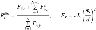 (1)where Iν is the specific
intensity of the star at a given wavelength/frequency, ℜ is the radius of the star, and
d is the
distance to the object. After a few trivial mathematical operations, for either of the
components of the binary system we obtain in terms of line depths
(1)where Iν is the specific
intensity of the star at a given wavelength/frequency, ℜ is the radius of the star, and
d is the
distance to the object. After a few trivial mathematical operations, for either of the
components of the binary system we obtain in terms of line depths  (2)where superscripts “th” and “c” refer to the
theoretical spectrum and continuum intensity, respectively, and subscript “comp” points to
the companion star. The factor fi = 1 / (1 +
α) is the light dilution factor briefly outlined in
Sect. 2.1. In this particular case of interpreting the individual binary components’
spectra independent of each other, nothing is known about the continuum intensity ratio of
the two stars and the light dilution factor fi is assumed to be
wavelength independent. In practice, each synthetic spectrum from the computed grid is
represented in the form of Eq. (2) and
compared to the observed disentangled spectrum on the scale of the latter.
(2)where superscripts “th” and “c” refer to the
theoretical spectrum and continuum intensity, respectively, and subscript “comp” points to
the companion star. The factor fi = 1 / (1 +
α) is the light dilution factor briefly outlined in
Sect. 2.1. In this particular case of interpreting the individual binary components’
spectra independent of each other, nothing is known about the continuum intensity ratio of
the two stars and the light dilution factor fi is assumed to be
wavelength independent. In practice, each synthetic spectrum from the computed grid is
represented in the form of Eq. (2) and
compared to the observed disentangled spectrum on the scale of the latter.
 |
Fig. 1 Diagram illustrating the algorithm implemented in the gssp_single software module. The two identical branches showed in the diagram indicate multiprocessing. See text for more details. |
Figure 1 illustrates the multiprocess algorithm implemented in the gssp_single software module. In the first step, the code reads in all necessary information provided by the user in the configuration file. We provide an example of the input file with detailed description of each entry in the Appendix. In the next step, the code sets up the grid and checks whether the required grid of atmosphere models is available. Should any of the models not exist, the user will be notified about the need to revise the input set up, and the detailed report is saved in one of the log-files. At this point, the observed spectrum can be optionally cross-correlated with the first synthetic spectrum from the grid, and the radial velocity (RV) is computed as the first order moment of the cross-correlation function. This way, the code accounts for a possible RV shift of the observed spectrum with respect to the laboratory wavelength, should the user request that. As soon as the grid has been set up (depending on the grid size, this might take up to half a minute of time), the code enters a multiprocessing mode and performs the actual calculations. The SynthV code is executed on each of the available CPUs and provides a synthetic spectrum for a given set of atmospheric parameters and in the requested wavelength range. The code computes specific line and continuum intensities for different positions of the stellar disk, thus providing an accurate treatment of the limb darkening effect. As soon as the spectrum is computed, a convolution program is executed to perform the disk integration and a convolution of the spectrum with projected rotational and macroturbulent velocities, and the resolving power of the instrument. The convolution code outputs the normalized synthetic spectrum as well as the line and continuum fluxes. The above described calculations may take from a few seconds up to a few minutes, depending on the spectral type and considered wavelength range. Once the convolved synthetic spectrum is released, there are two options for the code to contiue with (see Fig. 1): immediate comparison with the observations (the case of the spectrum of a single star), or dilution according to Eq. (2) and then the comparison with the observations (the case of the disentangled spectrum of a binary component). In either case, the final output of an individual process is the goodness of fit of the observed spectrum in terms of the χ2 merit function value, whereas the computed synthetic spectrum is immediately deleted. As soon as the calculations are finished on all the CPUs, the main process merges individual χ2 tables, finds the minimum in χ2, computes the best fit synthetic spectrum, and outputs the set of best fit parameters. We also provide the χ2 value corresponding to the 1σ uncertainty level computed from χ2 statistics and assuming normal distribution. This way, the projection of all data points on the parameter in question can be computed afterwards from the χ2 “master file”, and the 1σ uncertainties are obtained in a straightforward manner by fitting the χ2 distribution with a polynomial function and searching for its intersection points with the 1σ level in χ2 provided by the gssp_single module.
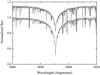 |
Fig. 2 Quality of the fit of the simulated data of KIC 11285625 (model 1b in Table A.1) with the gssp_single software package. The light dilution factor is 0.6/0.4 for the primary/secondary component. The simulated observed spectrum is shown with light grey lines, the black solid line refers to the best fit synthetic spectrum. The spectrum of the secondary was vertically shifted by a constant value for better visualization. |
The gssp_single module is reasonably fast and the final solution is obtained within 5–6 min by running the code on 8 CPUs, and assuming a typical grid size of 2000–3000 synthetic spectra and a 1000 Å wide wavelength range. The calculations may take a bit longer when fitting disentangled spectra, as there is an additional parameter (light dilution factor) to account for. The extra calculation time typically does not exceed 10% of the computation time in a single star spectrum mode, unless the grid resolution in the dilution factor is made unreasonably high.
The gssp_single software module is in fact an extension of the original version of the gssp code (Lehmann et al. 2011; Tkachenko et al. 2012) to make it compatible with the disentangled diluted spectra of stellar components in binary systems. The module was tested on simulated data of single stars; in addition, we refer the reader to the papers of Lehmann et al. (2011), Tkachenko et al. (2012, 2013a,b), Lampens et al. (2013), Pápics et al. (2014), Van Reeth et al. (2015) for several examples of the code application to the spectra of single stars, including some well studied objects like Vega.
For tests on the light diluted spectra of individual binary components, we decided not to simulate the spectra of arbitrary objects but instead used the binary components of KIC 6352430 (Pápics et al. 2013) and KIC 11285625 (Debosscher et al. 2013) as prototype stars. In our simulations, we assumed different dilution factors as well as different values of signal-to-noise ratio (S/N); the summary of the obtained results is given in Table A.1. Overall, we could recover the parameters of the input spectra assumed in all our simulations; the largest deviations, as well as 1σ uncertainties, have been observed for low S/N spectra. The quality of the fit to one pair of spectra is illustrated in Fig. 2. The only set up where we have encountered certain difficulties in recovering the assumed fundamental parameters refers to the case of peculiar stars (see Table A.4, the column indicated as “gssp_single”). In the simulations of KIC 11285625, we assumed an over/under-abundance of iron/silicon by 0.3/0.5 dex with respect to the global metallicity of the star for the primary/secondary component. For the KIC 6352430 system, the primary star was assumed to be peculiar in helium (+0.2 dex compared to the solar composition), whereas the secondary component was set up as a normal star with its own global metallicity. Since in the unconstrained fitting the spectra of individual components are considered separately, there is no way the results obtained for one of the components will influence the parameters of the companion. For this reason, we give no parameters for the secondary of KIC 6352430 in Table A.4 as they will be the same as the ones depicted in the second column of Table 4. We find that when a chemical element dominating the observed spectrum of the star shows significant over-/underabundance (iron in the primary of KIC 11285625), the global metallicity value gets affected and affects several other fundamental parameters as well (e.g., microturbulent velocity and surface gravity). Although this is not an unexpected result and the majority of the parameter values are still within 1σ uncertainties from the assumed values, the fact calls for a certain attention.
Results of the spectrum analysis of both stellar components of KIC 11285625 with the gssp_single and gssp_binary software packages (see text for details).
After testing the code on simulated data, we have applied the gssp_single module to the real disentangled spectra of both stellar components of the KIC 11285625, KIC 6352430, and KIC 4931738 systems. The latter object was also analyzed by Pápics et al. (2013) and consists of two stars of similar spectral types, luminosity classes, and rotation rates. The results of our analyses for all three binary systems are depicted in Tables 2–4, respectively, in the columns indicated as “gssp_single”. The parameters obtained by us are slightly different from those presented in the original studies, though the majority of the parameters still agree within the reported 1σ uncertainties. The obtained discrepancies for KIC 6352430 and KIC 4931738 may be associated with the fact that the microturbulent velocity was fixed to 2 km s-1 in the original study by Pápics et al. (2013), whereas it was set as a free parameter in our analysis. In addition, Pápics et al. (2013) assumed some dilution factor values coming from the preliminary fit of several observed composite spectral lines and used those to re-normalize the disentangled spectra of both binary components to the individual continua. In our case, both factors were set as free parameters and optimized along with other fundamental parameters for each of the components. As an example, in Fig. 3 we show the quality of the fit of the observed disentangled spectra of both components of the KIC 4931738 system by the best fit synthetic spectra computed from the parameters depicted in the first two columns of Table 4.
As it has been mentioned by Debosscher et al. (2013) in the original study, the spectroscopic data of KIC 11285625 have low S/N, which naturally propagates to the quality of the disentangled spectra. The secondary component, which contribution to the total light amounts to ~30%, suffered the most and its disentangled spectrum has rather low S/N and shows pronounced undulations in the local continuum. We anyway attempted to fit the spectrum of the secondary setting Teff, log g, ξ, v sin i, and [M/H] as free parameters in our analysis. We ended up with a clearly unreliable solution, in particular the value of log g was found to exceed 5.0 dex, which is not expected for the main-sequence star of spectral type F. Thus, following the procedure adopted in the original study of Debosscher et al. (2013), we fixed surface gravity of the secondary to the value obtained from the light curve solution, and optimized the four remaining fundamental parameters. Since the disentangled spectrum of the primary has higher S/N and suffered less from artifacts of spectral disentangling, we optimized all five fundamental parameters for this star, with the particular goal to compare the spectroscopic log g value with the one obtained from the light curve solution. The results of the analysis are summarized in Table 2 and show good agreement between the spectroscopic and photometric values of log g for the primary component, and overall agreement for all parameters of both binary components with the original study.
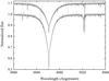 |
Fig. 3 Comparison between the observed disentangled spectra (light grey lines) of both stellar components of the KIC 4931738 system and the best fit synthetic spectra (black lines) computed with the gssp_single software module. The spectrum of the secondary was vertically shifted by a constant value for better visualization. |
 |
Fig. 4 Diagram illustrating the algorithm implemented in the gssp_binary software module. The two identical branches showed in the diagram indicate multiprocessing. See text for more details. |
2.3. GSSP_BINARY module
This module has been specifically designed for fitting disentangled spectra of both
binary components simultaneously. The procedure is in a sense similar to the one of
“constrained fitting” suggested by Tamajo et al.
(2011), were one assumes that the sum of the two light factors is identical to
unity, and thus the change in light dilution of one of the components affects the amount
of diluted light for the companion star. Instead of assuming wavelength-independent light
dilution for each of the components, we optimize the ratio of the radii of the binary
components which is obviously the same for both stars. Starting from the definition of
disentangled spectra of individual binary components given in Eq. (1), and dividing all terms on the right hand
side by the product between the continuum intensity of the secondary and its squared
radius, we obtain for the primary and secondary components of a binary 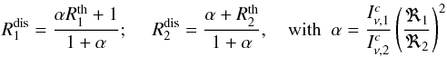 (3)or, in terms of line depths
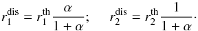 (4)Just as in the formulation of Tamajo et al. (2011), the sum of the two dilution
factors is identical to unity. By optimizing the ratio of the radii, we take into account
the wavelength-dependence of the light dilution factor through the ratio of continuum
intensities of the two stars. Obviously, any change in the atmospheric parameters of one
of the binary components will influence its continuum intensity, which will in turn affect
the light dilution factor for the companion star. In practice, disentangled spectra of two
binary components are analyzed simultaneously by scaling synthetic spectra from the
corresponding grids and comparing them to the observations on the scale of the latter.
(4)Just as in the formulation of Tamajo et al. (2011), the sum of the two dilution
factors is identical to unity. By optimizing the ratio of the radii, we take into account
the wavelength-dependence of the light dilution factor through the ratio of continuum
intensities of the two stars. Obviously, any change in the atmospheric parameters of one
of the binary components will influence its continuum intensity, which will in turn affect
the light dilution factor for the companion star. In practice, disentangled spectra of two
binary components are analyzed simultaneously by scaling synthetic spectra from the
corresponding grids and comparing them to the observations on the scale of the latter.
Figure 4 visualizes the algorithm implemented in the gssp_binary software module. Although the general principle is the same as for the gssp_single module, there are a number of differences that we discuss here in more detail. After reading all necessary information from the input file and checking the atmosphere models for availability, the code sets up the grid of synthetic spectra that need to be computed. As we have to deal with two components simultaneously, the algorithm of setting up the grid is different from the one implemented in the gssp_single module. To supply the code with maximum efficiency, we first build individual grids for both components of a binary system, and in the second step, a unique grid common for both stars is build by excluding any possible overlap in the parameters between the individual grids. This step is needed to avoid unnecessary repetitive calculations of theoretical spectra. For example, in the case of a binary system with two identical stars and thus identical initial parameter grids, only the primary’s grid will be computed and used for both binary components afterwards. The individual grids are used at this step to build all possible combinations of primary and secondary spectra, which will be processed at a later stage when looking for the best fit solution. For example, three grid points for each of the binary components will result in nine combinations to be processed in total, regardless of any possible overlap between the individual grids. As soon as the grids were set up (takes less than a minute of time), the code enters the parallel mode and starts the actual calculations of synthetic spectra as described in Sect. 2.1.
The normalized synthetic spectra as well as the corresponding continuum fluxes are stored in a database, which is an unformatted direct access Fortran 90 file. The advantage of using such a file over storing the data in an ASCII file is that any I/O operation with such a file is much faster as there is no conversion from machine code to a readable format. By storing the data in such a file we also avoid any possible problems with insufficient RAM memory, which might occur when keeping the (sometimes very large) grid of synthetic spectra in the memory. As soon as the database of spectra is produced, it is first made available to all CPUs involved in the calculations, and then the code enters the parallel mode for the second time. At this stage, every pre-build combination of primary and secondary spectra is processed, which involves dilution of both synthetic spectra extracted from the database and comparison with the observations on the scale of the latter. After processing all possible combinations, the χ2 files from individual CPUs are merged into a “master file”, and the best fit parameters and synthetic spectra for both binary components are released. Similar to the gssp_single software module, the 1σ level in χ2 is provided so that the corresponding uncertainties in all the parameters can be computed afterwards.
Despite a very large number of combinations that have to be processed, the gssp_binary module is reasonably fast. Assuming the same set up as the one described in Sect 2.1 – 8 CPUs and a 1000 Å wide wavelength range, – and ~500 synthetic spectra in a grid, the final solution is obtained within 15–20 min. To provide an estimate on the number of combinations, the above mentioned grid of ~500 spectra coupled with only three grid points in the radii ratio results in about 200 000 combinations to be processed by the code.
The gssp_binary software module has been extensively tested by us both on simulated and real spectra of double-lined spectroscopic binary stars. Similar to the tests described in Sect 2.1, KIC 11285625 and KIC 6352430 were used as prototype stars for our simulations, and the observed disentangled spectra of the KIC 6352430, KIC 11285625, and KIC 4931738 systems were used to test the code on data of real binary systems. The results of the code application to the simulated data are summarized in Table A.2. Similar to the tests performed in Sect. 2.1, we also applied the gssp_binary module to the simulated spectra showing anomalies in the abundances of certain chemical elements. The results of this application are summarized in Table A.4, in the columns indicated as “gssp_binary”. The conclusions from our test runs on the simulated data are essentially the same as in Sect. 2.1: i) the input parameters are recovered in the majority of the cases; ii) the largest deviations from the input values as well as the largest uncertainties are observed for low S/N data; and iii) anomalies in the abundances of chemical elements dominating the observed spectrum significantly affect the determination of the global metallicity, which in turn triggers deviations in other fundamental parameters of the star. Since in the constrained fitting mode spectra of both binary components are fitted simultaneously, any changes in the parameters of one of the components will likely affect the parameter determination for the companion star, due to changes in the light dilution factor. The quality of the fit of the simulated data is essentially the same as the one shown in Fig. 2, for which reason it is not illustrated here.
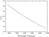 |
Fig. 5 Ratio of the continuum intensity of the primary to the one of the secondary in the KIC 6352430 system. The models were computed for the fundamental parameters listed in the last two columns of Table 3. |
The results of the application of the gssp_binary software module to the real spectra of KIC 11285625, KIC 6352430, and KIC 4931738 are summarized in Tables 2–4, respectively (column indicated as “gssp_binary”). Significant deviations are observed for some of the parameters from those obtained with the gssp_single module (unconstrained fitting) for the KIC 11285625 system. This is likely explained by the insufficient quality of the data for the secondary component, whose parameter determination in turn affects the solution for the primary component. Indeed, the results of the unconstrained fitting with the gssp_single module (first two columns in Table 2) suggest the sum of the dilution factors to be well below unity. According to the definition of disentangled spectra from Eq. (3), this sum is identical to unity in the constrained fitting mode, thus the gssp_binary code is in a sense forced to look for an alternative solution that would satisfy the above mentioned criterion. The change in the light dilution of each of the components in turn triggers the differences in fundamental parameters compared to the gssp_single solution.
Certain deviations in the metallicity and effective temperature of the secondary are observed for the KIC 6352430 when compared to the solution obtained with the gssp_single module. Given that the latter suggests unity for the sum of the light factors, the observed discrepancies are likely due to wavelength dependence of the light dilution factors. Indeed, the primary component is twice as hot as its companion star, suggesting that the continuum intensity ratio might vary significantly within the considered 1000 Å wide wavelength range. Figure 5 illustrates the variation of the ratio of the continuum intensity of the primary to the one of the secondary as a function of wavelength, in the range between 4750 and 5750 Å. The ratio changes from ~4.9 at λλ 4750 Å to ~3.9 at λλ 5750 Å. For comparison, the variation in the same quantity for the KIC 11285625 system consisting of two similar stars (see Table 2) does not exceed 0.2% of the value of 0.955 measured at 5250 Å.
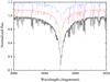 |
Fig. 6 Quality of the fit of the simulated composite spectrum of KIC 11285625 (model 1a in Table A.3) with the gssp_composite software package. The radii ratio is 1.45, in agreement with the value reported by Debosscher et al. (2013). The simulated observed spectrum is shown with a light grey line, the black solid line refers to the best fit synthetic spectrum, the individual spectra of the primary/secondary are shown by the red dashed/blue dotted lines. The individual, RV-shifted spectra of the binary components were vertically shifted for better visualization. |
2.4. GSSP_COMPOSITE module
The gssp_composite software module was specifically designed for fitting
composite spectra of double-lined spectroscopic binary systems. We refer the reader to
Fig. 4 and the description there for details on the
implemented algorithm as it is very similar to the one implemented in the
gssp_binary module. The only two differences in the gssp_composite
algorithm are: i) there is a possibility to set the radial velocities of individual binary
components as free parameters; and ii) instead of comparing theoretical spectra to the
disentangled observed spectra of both components, all possible combinations of synthetic
primary and secondary spectra from the computed grid are used to build composite
theoretical spectra of a binary which are then compared to the observed spectrum on the
scale of the latter. Composite theoretical spectra are represented in the form
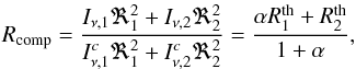 (5)where α is defined the same way
as in Eq. (3).
(5)where α is defined the same way
as in Eq. (3).
We have tested the gssp_composite module on simulated composite spectra of binary stars, where the KIC 11285625 and KIC 6352430 binaries were again used as the prototype systems. The results of our test runs are summarized in Table A.3; quality of the fit to one of the spectra is illustrated in Fig. 6. As for the two previously described software packages, we could recover the input parameters for the majority of the models. However, we find that a combination of low S/N and a small light contribution from either of the binary components becomes a real bottleneck for fitting the composite spectrum of a binary system. The only reasonable estimates in this case are obtained for the radial velocities of stars, provided both components show a sufficient amount of metal lines in their spectra and the lines are well separated in velocity space. For the rest of the parameters fitting the composite spectra fails, for which reason there are no entries for the secondary components of KIC 11285625 and KIC 6352430 in Table A.3 at S/N of 60 and large values of the radii ratio. An assumption that one or both stellar components of a binary show significant anomalies in their spectra leads to the same results than have been obtained with the gssp_binary software package (see Sect. 2.2). For a limited amount of models, we also performed test runs assuming that spectral lines of individual spectral components overlap in the velocity space. To our surprise, even in this case all initially assumed fundamental parameters could be reasonably recovered, provided sufficiently high S/N (>150) of the input data. No application of the gssp_composite module was done to real data of double-lined spectroscopic binaries, however. The reason is that the individual composite observed spectra of all three systems (KIC 11285625, KIC 6352430, and KIC 4931738) considered in our work have S/N that are too low for the method to be robust.
The gssp_composite software module is much more time consuming than the two previously described modules. The reason is quite simple: assuming a set up that includes calculation of ~500 synthetic spectra, a 1000 Å wide wavelength range, 8 CPUs, and three grid points in RV for each of the components, the total number of the grid combinations to be processed by the code is close to 1 500 000. This is a factor of almost 10 more than for the same set up in the gssp_binary module, which transforms into about an hour of computation time.
3. Summary
In this paper, we have presented a Fortran 90 code for spectrum analysis of single stars and double-lined spectroscopic binary systems. The code makes use of the OpenMPI distribution and runs in parallel mode.
There are three independent software modules included, each one is designed for the application to a certain type of data. The gssp_single module can be applied to the spectroscopic data of single stars as well as to the disentangled, light diluted spectra of spectroscopic binary components. In the latter case, the spectra of the stars are interpreted independently of each other and the code assumes wavelength-independent light dilution for each of the stars. The two other modules, gssp_binary and gssp_composite, are specifically designed to fit the spectra of double-lined spectroscopic binary systems. Where the first module analyzes disentangled spectra, the second one focuses on direct fitting of the composite spectra. The gssp_binary module fits disentangled spectra of both binary components simultaneously and assumes that the light dilution factor of each of the components is a function of wavelength. The light factors are replaced in the grid by the ratio of the components’ radii, which is obviously the same for both stars. This way, an additional constraint is put on individual light factors, namely their sum should equal unity at each considered wavelength. The algorithm implemented in the gssp_composite module is essentially the same, except that composite spectra are fitted instead of disentangled ones. Radial velocities of the individual stellar components can also be included into the fit if necessary.
No matter which module is used for the spectroscopic analysis, we note that it is advisable to start from reasonably coarse grid(s) which would cover large parameter ranges. This step is absolutely necessary to finally find a global minimum solution but not to be stuck in a local minimum. For example, it is important to keep the range in the effective temperature that would cover the entire range of spectral type in question. The full ranges for the surface gravity and the metallicity currently available in the LLmodels library of atmosphere models (see Table 1 for details) would be a good choice for the initial run. However, the step sizes should be set to rather large values (e.g., 0.5 and 0.4 dex for log g and [M/H, respectively]), to keep the calculation time at a reasonable level. As soon as the first, coarse grid solution is obtained, the parameter ranges should be gradually narrowed down, also making the grid finer. To speed up the calculations with the gssp_composite module, we would recommend making a prior estimate of the radial velocities of the individual binary components (if at all possible) and to keep them fixed throughout the analysis.
The gssp_single and gssp_binary software modules are quite fast and the calculation time is reasonable even when the code is run on a quad core desktop or laptop. If the disentangled spectra of both binary components are available, and the difference in spectral types of the two binary components is not large, we suggest starting the analysis with the unconstrained fitting mode implemented in the gssp_single module. This way, very good initial guesses can be obtained for both stellar components of a binary system within short time. With a good initial grid setup for the gssp_binary module, the physically more correct solution for both binary components can be obtained within a limited amount of time. The disentangled spectra of the components of a binary systems can be obtained in different ways; the most widely used methodologies and codes are those presented by Simon & Sturm (1994, spectral disentangling in wavelength domain), Hadrava (1995) and Ilijic et al. (2004, Fourier spectral disentangling). The gssp_composite module is more time consuming than the two previous ones, thus we suggest using it when i) very good quality data (S/N> 150) are available; ii) good initial guesses for the fitted parameters are provided; and iii) at least some of the parameters can be fixed, e.g., from the light curve solution.
Test runs of all three modules on the simulated data have shown that all input parameters are well recovered in the majority of cases. For the fitting of disentangled spectra, S/N ≥ 100 is likely to be sufficient for decent analysis, whereas the composite spectrum fitting generally requires a S/N above 150. The gssp software package is also suitable for the analysis of peculiar stars, though it should be noted that the global metallicity of the stars can be significantly under/overestimated should the peculiarity concern one of the dominant chemical elements in the spectrum.
The application to real data has shown that for binary systems consisting of two stars with significantly different spectral types, the unconstrained fitting is likely to deliver not entirely correct parameters. This is due to significant variations of the light dilution factor with wavelength, as was the case for the KIC 6352430 system analyzed in this study.
In future, we plan to extend the software to the analysis of hot stellar objects (early O-B spectral types) by including non-LTE effects into the calculation of synthetic spectra. We will use the so-called hybrid approach assuming non-LTE radiative transfer calculations for chemical elements of interest, based on classical LTE atmosphere models. The justification of such approach is discussed in Nieva & Przybilla (2007). The implementation is rather straightforward and consists of using pre-computed departure coefficients from LTE in the SynthV radiative transfer code. The coefficients can be computed based on the LTE atmosphere models with software such as the tlusty3 (Hubeny 1988) code. We plan to perform such calculations for the entire hot part of our grid of LLmodels atmosphere models, so that non-LTE spectrum synthesis can be done for any relevant model when it is needed. Computing departure coefficients (including
elements with complex atomic structure) for a rather large subgrid of atmosphere models is a quite time-consuming procedure, which may take up to several months of computation time. This prevents us from including the non-LTE option in the current version of the software release.
Acknowledgments
The author is grateful to Prof. Vadim Tsymbal for providing the SynthV radiative transfer code and for the support in using it. The whole IvS team and Dr. Holger Lehmann from Thüringer Landessternwarte Tautenburg are thanked for valuable discussions; Dr. Peter Papics and Dr. Katrijn Clemer are acknowledged for careful reading of the paper and providing a valuable feedback. The author particularly acknowledges Prof. Dr. Conny Aerts for encouraging him to develop the gssp software package. Finally, the author wants to thank the referee for careful reading of the manuscript and providing valuable comments that helped to improve the paper. The research leading to these results has received funding from the European Community’s Seventh Framework Programme FP7- SPACE-2011-1, project number 312844 (SPACEINN).
References
- Andrássy, R., &Spruit, H. C. 2015, A&A, 579, A122 [NASA ADS] [CrossRef] [EDP Sciences] [Google Scholar]
- Auvergne, M., Bodin, P., Boisnard, L., et al. 2009, A&A, 506, 411 [NASA ADS] [CrossRef] [EDP Sciences] [Google Scholar]
- Berdyugina, S. V. 1994, Astron. Lett., 20, 796 [NASA ADS] [Google Scholar]
- Chiosi, C., &Maeder, A. 1986, ARA&A, 24, 329 [NASA ADS] [CrossRef] [Google Scholar]
- Debosscher, J., Aerts, C., Tkachenko, A., et al. 2013, A&A, 556, A56 [NASA ADS] [CrossRef] [EDP Sciences] [Google Scholar]
- Delgado Mena, E., Bertrán de Lis, S.,Adibekyan, V. Z., et al. 2015, A&A, 576, A69 [NASA ADS] [CrossRef] [EDP Sciences] [Google Scholar]
- Gilliland, R. L., Brown, T. M.,Christensen-Dalsgaard, J., et al. 2010, PASP, 122, 131 [NASA ADS] [CrossRef] [Google Scholar]
- Gustafsson, B., Edvardsson, B., Eriksson, K., et al. 2008, A&A, 486, 951 [NASA ADS] [CrossRef] [EDP Sciences] [Google Scholar]
- Hadrava, P. 1995, A&AS, 114, 393 [NASA ADS] [Google Scholar]
- Hubeny, I. 1988, Comput. Phys. Comm., 52, 103 [Google Scholar]
- Ilijic, S., Hensberge, H., Pavlovski, K., &Freyhammer, L. M. 2004, Spectroscopically and Spatially Resolving the Components of the Close Binary Stars, 318, 111 [Google Scholar]
- Kochukhov, O., &Bagnulo, S. 2006, A&A, 450, 763 [NASA ADS] [CrossRef] [EDP Sciences] [Google Scholar]
- Kupka, F., Piskunov, N., Ryabchikova, T. A.,Stempels, H. C., & Weiss, W. W. 1999, A&AS, 138, 119 [NASA ADS] [CrossRef] [EDP Sciences] [MathSciNet] [PubMed] [Google Scholar]
- Kurucz, R. 1993, ATLAS9 Stellar Atmosphere Programs and 2 km s-1 grid. Kurucz CD-ROM No. 13 (Cambridge, Mass.: Smithsonian Astrophysical Observatory) [Google Scholar]
- Lampens, P., Tkachenko, A., Lehmann, H., et al. 2013, A&A, 549, A104 [NASA ADS] [CrossRef] [EDP Sciences] [Google Scholar]
- Lehmann, H., Tkachenko, A., Semaan, T., et al. 2011, A&A, 526, A124 [NASA ADS] [CrossRef] [EDP Sciences] [Google Scholar]
- Maeder, A. 1983a, A&A, 120, 113 [NASA ADS] [Google Scholar]
- Maeder, A. 1983b, A&A, 120, 130 [NASA ADS] [Google Scholar]
- Massey, P. 2003, ARA&A, 41, 15 [NASA ADS] [CrossRef] [Google Scholar]
- Nieva, M. F., &Przybilla, N. 2007, A&A, 467, 295 [NASA ADS] [CrossRef] [EDP Sciences] [Google Scholar]
- Pápics, P. I.,Tkachenko, A., Aerts, C., et al. 2013, A&A, 553, A127 [NASA ADS] [CrossRef] [EDP Sciences] [Google Scholar]
- Pápics, P. I.,Moravveji, E., Aerts, C., et al. 2014, A&A, 570, A8 [NASA ADS] [CrossRef] [EDP Sciences] [Google Scholar]
- Perryman, M. A. C., de Boer, K. S.,Gilmore, G., et al. 2001, A&A, 369, 339 [NASA ADS] [CrossRef] [EDP Sciences] [Google Scholar]
- Pöhnl, H., Maitzen, H. M., &Paunzen, E. 2003, A&A, 402, 247 [NASA ADS] [CrossRef] [EDP Sciences] [Google Scholar]
- Rauer, H., Catala, C., Aerts, C., et al. 2014, Exp. Astron., 38, 249 [NASA ADS] [CrossRef] [Google Scholar]
- Ricker, G. R., Winn, J. N.,Vanderspek, R., et al. 2014, Proc. SPIE, 9143, 914320 [Google Scholar]
- Simon, K. P., &Sturm, E. 1994, A&A, 281, 286 [NASA ADS] [Google Scholar]
- Shulyak, D., Tsymbal, V., Ryabchikova, T. et al. 2004, A&A, 428, 993 [NASA ADS] [CrossRef] [EDP Sciences] [Google Scholar]
- Soderblom, D. R. 2015, Astrophys. Space Sci. Proc., 39, 3 [NASA ADS] [CrossRef] [Google Scholar]
- Tamajo, E., Pavlovski, K., &Southworth, J. 2011, A&A, 526, A76 [NASA ADS] [CrossRef] [EDP Sciences] [Google Scholar]
- Tkachenko, A., Lehmann, H., Smalley, B., Debosscher, J., &Aerts, C. 2012, MNRAS, 422, 2960 [NASA ADS] [CrossRef] [Google Scholar]
- Tkachenko, A., Lehmann, H., Smalley, B., &Uytterhoeven, K. 2013a, MNRAS, 431, 3685 [NASA ADS] [CrossRef] [Google Scholar]
- Tkachenko, A., Aerts, C., Yakushechkin, A., et al. 2013b, A&A, 556, A52 [NASA ADS] [CrossRef] [EDP Sciences] [Google Scholar]
- Tsymbal, V. 1996, ASP Conf. Ser., 108, 198 [Google Scholar]
- Valenti, J. A., &Piskunov, N. 1996, A&AS, 118, 595 [NASA ADS] [CrossRef] [EDP Sciences] [Google Scholar]
- Van Reeth, T., Tkachenko, A., Aerts, C., et al. 2015, A&A, 574, A17 [NASA ADS] [CrossRef] [EDP Sciences] [Google Scholar]
- Walker, G., Matthews, J., Kuschnig, R., et al. 2003, PASP, 115, 1023 [NASA ADS] [CrossRef] [Google Scholar]
Appendix A: Results of the analysis of simulated spectra
Results of the application of the gssp_single software module to the simulated data of KIC 11285625 (model 1) and KIC 6352430 (model 2) assuming different S/N and dilution factors.
Results of the analysis of simulated spectra of two binary systems, assuming peculiar abundances of Fe/Si for the primary/secondary of KIC 11285625, and of He for the primary of KIC 6352430.
Appendix B: The GSSP package: Installation, running, and configurations files
Appendix B.1: Installation and running
The Grid Search in Stellar Parameters (gssp) package is a compilation of three separate modules, each one designed for the analysis of a certain type of spectroscopic data. The code makes use of an open source Message Passing Interface (OpenMPI) implementation, which has to be installed along with the Intel Fortran Compiler on the machine where the gssp code is supposed to run. The version of OpenMPI 1.3.3 from July 14th, 2009 is suitable; any stable version of the Intel Compiler is good but the release should not be older than the one from the 12th of February, 2012 (version 12.1.3).
The code compiles with the following simple command:
mpif90 -o executable_name *.f*
where “executable_name” is the name of an executable file (can be anything the user likes). The compilation command is the same for all the package modules. For the compilation to be successful, one needs to run the compilation command twice. During the first run, the GSSP_module.f90 file is processed and the *.mod file with the corresponding name is produced. This file contains the majority of declarations as well as some other relevant information for other subroutines. During the second run of the compilation command, the compiler gets the information from the *.mod file and all remaining Fortran source files get successfully processed.
To run the code, one need to use the following command:
mpirun-nN[-hostfileHost˙file˙name]
executable˙nameInput˙file˙name
where N is the number of CPUs. The arguments given in brackets are optional and not needed when the code is run on a single machine with multiple-cores. The arguments become useful when the code runs on a cluster PC with several nodes involved. The host file contains information about the names of the individual nodes on which the code will be running, and the number of CPUs on each of those nodes. An example of such hostfile is given below.
node01 slots = 8
node02 slots = 8
node03 slots = 8
node04 slots = 8
node05 slots = 8.
Appendix B.2: Configuration files
In this section, we discuss the structure of the input files for all three modules of the gssp package. Our intention is to give as much detail as needed for each entry from those files.
The gssp_single module
Teff_start Teff_step Teff_end ! effective temperature range (K)
logg_start logg_step logg_end ! log surface gravity range (dex)
vmicro_start vmicro_step vmicro_end ! microturbulent velocity range (km s-1)
vsini_start vsini_step vsini_end ! projected rotational velocity range (km s-1)
dilution_flag factor_start factor_step factor_end ! light dilution flag and light dilution factor range
abund_flag [M/H]_start [M/H]_step [M/H]_end ! abundance flag and metallicity range (dex)
element_id abund_start abund_step abund_end ! chemical element id (e.g., Fe or He) and abundance range
vmacro resolution ! macroturbulent velocity (km s-1) and resolving power
abundance_path ! absolute path to the abundance table(s)
model_path ! absolute path to the library of atmosphere models
vmicro_model mass_model ! atmosphere model microturbulent velocity (km s-1) and mass (M⊙)
model_comp_flag ! atmosphere model chemical composition flag (ST, CNm, or CNh)
nranges wave_step mode ! Number of wavelength regions, wavelength step (Å), operational mode flag
spectrum_path ! Path to the observed spectrum
RV_factor contin_factor RV RV_flag ! RV scaling factor, continuum cutoff factor, RV value, RV option
wave_start wave_end ! wavelength range(s) in Å
wave_start wave_end.
The first four entries in the configuration file set up the ranges and step sizes for the effective temperature (Teff), logarithm of surface gravity (log g), microturbulent velocity (ξ), and projected rotational velocity (v sin i). For example,
6800 100 7200 ! effective temperature range (K)
2.9 0.2 3.9 ! log surface gravity range (dex)
2.8 0.4 4.4 ! microturbulent velocity range (km s-1)
35 5 50 ! projected rotational velocity range (km s-1).
The next two entries set up the grid ranges for the light dilution factor and the global metallicity [M/H] of the star. In both cases, certain flags precede the parameter ranges. Should the light dilution option be used in the calculations (in case of the analysis of disentangled spectra of binary components), the value “adjust” must be set for the dilution_flag parameter. Otherwise (analysis of single stars), the value of the dilution_flag parameter needs to be set to “skip”. Similarly, the abund_flag takes one of the two following values: “skip” or “adjust”. The “skip” option assumes that the global metallicity of the star can be optimized along with the other fundamental parameters (Teff, log g, ξ, and v sin i). In this case, individual abundances of all metals will be scaled by the same amount. The “adjust” option assumes that the metallicity parameter will be replaced in a grid by a chemical element (any, except hydrogen) abundance. The individual abundances are optimized for one chemical element at the time; the metallicity value [M/H] must be fixed while all other fundamental parameters can be kept free. For example,
adjust 0.6 0.1 1.0 ! light dilution flag and light dilution factor range
skip −0.1 0.1 0.2 ! abundance flag and metallicity range (dex).
For detailed chemical composition analysis of the star, we recommend to do the analysis in two steps: 1) optimizing the global metallicity value together with the other four (and, optionally, the light dilution factor) fundamental parameters; 2) fixing the metallicity to the value derived in the first step and optimizing individual abundances along with the other parameters.
The entry element_id abund_start abund_step abund_end is only relevant when the individual abundances have to be optimized. Below are the entry examples for Fe:
Fe −4.59 0.05 −4.39 ! chemical element id (e.g., Fe or He) and abundance range
and for He
He 0.0783 0.0005 0.0813 ! chemical element id (e.g., Fe or He) and abundance range
The element_id parameter refers to the element designation (e.g., Fe for iron, He for helium); the numbers give the range and a step width. Should the value of the abund_flag parameter be set to “skip”, the entire entry will be ignored by the code. We note that the abundances of all metals are in logarithmic scale, but those of hydrogen and helium are not. Thus, when optimizing the helium abundance, we note that these are positive values and the range should always be given from the smallest to the largest value (see example above).
The vmacro resolution entry does not need any specific remarks as it gives the values of macroturbulent velocity (in km s-1) and of the resolving power of the instrument. Both parameters are used by the convolution code to add the corresponding broadening to synthetic spectra. For example,
0.0 32 000 ! macroturbulent velocity (km s-1) and resolving power.
The next two entries, abundance_path and model_path, specify absolute paths to a file with individual abundances and to the folder containing atmosphere models, respectively. For example:
/home/UserName/Abundance_table.abn ! absolute path to the abundance table(s)
/home/UserName/LLmodels/ ! absolute path to the library of atmosphere models
or
/home/UserName/abundances/ ! absolute path to the abundance table(s)
/home/UserName/LLmodels/ ! absolute path to the library of atmosphere models.
A library of LLmodels atmosphere models is included into the gssp package; the library of interpolated Kurucz models with the resolution matching the one of the LLmodels grid is provided upon request. The file with the individual abundances can have any name but the extension *.abn is fixed. The program will not run in the abund_flag = adjust mode if the file name with individual abundances is not provided. At the same time, the global metallicity parameter [M/H] must be fixed when the name of *.abn file is provided in the configuration file. Whenever [M/H] is set as a free parameter, the path should be provided to the folder that contains abundance tables corresponding to different global metallicity values (e.g., /home/UserName/abundances/). These global metallicity abundance tables have been pre-computed and are included in the gssp package distribution. Summarizing, the abundance_path parameter is closely connected to the [M/H] parameter (whether it is free or not) and to the abund_flag:
-
[M/H] is a free parameter: the absolute path to the folder with pre-computed chemical composition tables should be provided (e.g., /home/UserName/abundances/). Providing the name of a *.abn file in this case will result in an error message.
-
[M/H] is fixed and abund_flag = skip: the other four fundamental parameters (Teff, log g, ξ, and v sin i) and (optionally) the dilution factor can be optimized based on the provided table with individual abundances. There are two options here: either one provides a path to the file that contains specific abundances (e.g., /home/UserName/Abundance_table.abn), or a path to the folder containing pre-computed abundance tables corresponding to different metallicity values (e.g., /home/UserName/abundances/).
-
[M/H] is fixed and abund_flag = adjust: the other four fundamental parameters (Teff, log g, ξ, and v sin i) and (optionally) the dilution factor can be optimized simultaneously with the individual abundances (one element at the time). In this case, a path to the file that contains specific elemental abundances has to be provided (e.g., /home/UserName/Abundance_table.abn). Otherwise, the code will give an error message.
The next two entries in the configuration file, vmicro_model mass_model and model_comp_flag, set the values of the atmosphere model microturbulent velocity (in km s-1) and mass (M⊙), and the value of the atmosphere model chemical composition flag. For example,:
2 1 ! atmosphere model microturbulent velocity (km s-1) and mass (M⊙)
ST ! atmosphere model chemical composition flag (ST, CNm, or CNh)
All atmosphere models in the provided LLmodels grid have been computed for the fixed value of the microturbulent velocity of 2 km s-1. However, the user is free to use his/her own grid of models (in Kurucz format!) computed for a different value of the microturbulence. The other two parameters, mass_model and model_comp_flag, were specifically included should the user want to use marcs4 (Gustafsson et al. 2008) atmosphere models computed assuming a different mass and/or chemical composition. Should the user choose to use the provided grid of the LLmodels atmosphere models, both parameters must be fixed to the values given in the above example. When using spherical marcs models, one has to be aware that a hybrid approach is adopted in the spectrum analysis – spherical models and a plane-parallel radiative transfer formalism in the spectrum synthesis code. The parameter model_comp_flag takes one of the three following values: “ST” (stands for standard), “CNm” (stands for moderately CN-cycled), or “CNh” (stands for heavily CN-cycled). The “standard” mixture reflects the typical elemental abundance ratios in stars as a function of metallicity in the solar neighborhood. Two types of CN-cycled marcs models reflect different carbon isotopic ratios (12C/13C; see marcs website for details).
The nranges wave_step mode entry sets the number of wavelength ranges to be considered in the analysis, the wavelength step width (in Å), and the operational mode. For example:
2 0.0376 fit ! Number of wavelength regions, wavelength step (Å), and operational mode flag
The mode parameter can be assigned one of the following key words: “fit” or “grid”. The first, fitting mode, assumes that the observed spectrum is provided (see below) and a grid of synthetic spectra will be fitted to it. The quality of the fit is evaluated based on the χ2-criterion; the χ2 distributions are provided for all free parameters as an output (see below). The number of wavelength regions can be set to any integer number, the ranges themselves are provided in the configuration file. The value of the step width in wavelength is ignored in this case, and is computed directly from the observations (see below). The second value that the mode parameter can take is “grid”. In this case, no fitting to the observations is performed and a grid of synthetic spectra is computed in the required parameter space. This option assumes that the spectra are calculated in a single wavelength range, thus the number of wavelength ranges (nranges) should be set to unity. The step width in wavelength is also an important parameter in this case, as it defines the wavelength grid for synthetic spectra.
The spectrum_path entry provides a path (absolute or relative) to the observed spectrum. This entry in the configuration file will be ignored should the user run the code in the “grid” mode. For example:
home/UserName/Obs_spectrum.dat ! Path to the observed spectrum.
The observed spectrum is an important part of the fitting mode, thus an error message will be given when the spectrum is not provided but the operational mode is set to “fit”. The observed spectrum should be provided in a two-column ASCII file, where the first and the second columns refer to wavelength (in Å, linear scale) and normalized flux, respectively. We note that the wavelength scale of the observed spectrum should be equidistant. The step width in wavelength that will be used for the calculation of synthetic spectra is computed from the observations.
The RV_factor contin_factor RV RV_flag entry is relevant when the fitting operational mode is chosen. Otherwise, it will be ignored by the code. For example:
0.50 0.99 −35.5 fixed ! RV scaling factor, continuum cutoff factor, RV value, RV option.
The gssp_single module has an option to compute the cross-correlation function (CCF) between the observations and the first synthetic spectrum from the grid. The CCF will be computed when the RV_flag is assigned the key word “adjust”. Otherwise (RV_flag = fixed), the code assumes that the radial velocity of the observed spectrum is known and the RV value preceding the RV_flag in the configuration file (−35.5 km s-1 in the example above) is used to correct the observations. Should the CCF calculation be requested by the user, the RV of the observed spectrum is determined as the first order moment of the CCF. The velocity range in the CCF from which the radial velocity is computed is defined by the user in a parameterized way. The control parameter is RV_factor (takes the value of 0.5 in the example above), which sets the intensity cut limit in the normalized to a unity CCF function. We strongly recommend to use a value of 0.5 or slightly larger, which in practice means that the CCF will be cut at its half maximum intensity and the part above will be used to compute the first order moment. Finally, the contin_factor parameter takes a value between 0 and 1 and reflects the cutoff value in the normalized observed flux. All flux points above this value (0.99 in the example above) will be taken into account in the calculation of the global continuum correction factor. The information about the global continuum position is taken from the synthetic spectra; the factor is computed by means of the least-squares fit of the observations to the theoretical spectrum. In practice, the value of this parameter should be fairly large (between 0.95 and 1.0) to ensure that mainly the continuum points are taken into account and the result is not biased by the inclusion of weak spectral lines. Should the user not want to do any continuum correction, the parameter can be set to some unreliably large value (e.g., 10 000), which will force the correction factor to be identical to unity.
The wave_start wave_end entry refers to the wavelength range to be considered in the analysis. The number of entries should be equal to the number of wavelength regions (nranges) specified earlier in the configuration file (see above). For example:
4750 5000 ! wavelength range(s) in Å
5200 5700.
Only one wavelength range can be provided when the operational mode is set to “grid”. In the fitting mode, the number of wavelength regions is not limited, which makes the fitting of individual lines in the spectrum possible.
The gssp_binary module
number_components ! number of stellar components
Teff_start 1 Teff_step 1 Teff_end 1 Teff_start 2 Teff_step 2 Teff_end 2
logg_start 1 logg_step 1 logg_end 1 logg_start 2 logg_step 2 logg_end 2
vmicro_start 1 vmicro_step 1 vmicro_end 1 vmicro_start 2 vmicro_step 2 vmicro_end 2
vsini_start 1 vsini_step 1 vsini_end 1 vsini_start 2 vsini_step 2 vsini_end 2
abund_flag 1 [M/H]_start 1 [M/H]_step 1 [M/H]_end 1 abund_flag 2 [M/H]_start 2 [M/H]_step 2 [M/H]_end 2
element_id 1 abund_start 1 abund_step 1 abund_end 1 element_id 2 abund_start 2 abund_step 2 abund_end 2
radii_ratio_start radii_ratio_step radii_ratio_end ! ratio of the components’ radii
vmacro 1 vmacro 2 resolution
abundance_path 1
abundance_path 2
model_path
vmicro_model mass_model
model_comp_flag
nranges ! Number of wavelength regions to be considered in the analysis
spectrum_path1 ! Path to the disentangled observed spectrum of the primary
spectrum_path2 ! Path to the disentangled observed spectrum of the secondary
RV_factor 1 RV 1 RV_flag 1 contin_factor 1 RV_factor 2 RV 2 RV_flag 2 contin_factor 2
wave_start wave_end
wave_start wave_end.
Since the structure of the configuration file itself and the meaning of the input parameters are very similar to those of the gssp_single module, we only discuss extra parameters specific to the gssp_binary software module. In the above example of the configuration file, superscripts “1” and “2” refer to the primary and secondary components of a binary, respectively.
The number_components refers to the number of stellar components in the system. Currently, the value of this parameter always has to be set to 2.
radii_ratio_start radii_ratio_step radii_ratio_end is another entry in the configuration file that needs some attention. The entry refers to the binary components’ radii ratio and is obviously the same for both stellar components. Depending on the binary system considered, this ratio can have values close to one or above ten.
The gssp_composite module
number_components ! number of stellar components
Teff_start 1 Teff_step 1 Teff_end 1 Teff_start 2 Teff_step 2 Teff_end 2
logg_start 1 logg_step 1 logg_end 1 logg_start 2 logg_step 2 logg_end 2
vmicro_start 1 vmicro_step 1 vmicro_end 1 vmicro_start 2 vmicro_step 2 vmicro_end 2
vsini_start 1 vsini_step 1 vsini_end 1 vsini_start 2 vsini_step 2 vsini_end 2
abund_flag 1 [M/H]_start 1 [M/H]_step 1 [M/H]_end 1 abund_flag 2 [M/H]_start 2 [M/H]_step 2 [M/H]_end 2
element_id 1 abund_start 1 abund_step 1 abund_end 1 element_id 2 abund_start 2 abund_step 2 abund_end 2
radii_ratio_start radii_ratio_step radii_ratio_end ! ratio of the components’ radii
RV_start1 RV_step1 RV_end1 RV_start2 RV_step2 RV_end2 ! radial velocity ranges (km s-1)
vmacro 1 vmacro 2 resolution
abundance_path 1
abundance_path 2
model_path
vmicro_model mass_model
model_comp_flag
nranges ! Number of wavelength regions to be considered in the analysis
spectrum_path ! Path to the composite observed spectrum of the binary system
contin_factor ! continuum cutoff factor
wave_start wave_end
wave_start wave_end.
The meaning of the majority of the entries is the same as in the gssp_single and gssp_binary modules, thus a detailed discussion is omitted here.
RV_start1 RV_step1 RV_end1 RV_start2 RV_step2 RV_end2 is the only entry that requires some attention as it is newer than all the previously discussed entries. The entry obviously refers to the individual component grids in radial velocities (in km s-1). Should the user want to fix the RV of either of the component stars, the RV_start parameter must be set equal to the RV_end parameter.
Appendix B.3: Output files
All output files are stored in the “output_files” folder that is located in the local work directory and is created automatically by the code. The first important output file has the name “ModelOverview.txt”. Whenever the user is out of the parameter range provided by the library of atmosphere models, the code will exit with an error message, referring the user to this file. It gives an overview of all models that do (or do not) exist in the specified parameter space. The file has the following structure:
[M/H] = -0.1 Teff = 6800.0 logg = 2.90 Vmicro = 2.0 Mass = 1.0 OK
[M/H] = -0.1 Teff = 6800.0 logg = 3.10 Vmicro = 2.0 Mass = 1.0 OK
[M/H] = -0.1 Teff = 6800.0 logg = 3.30 Vmicro = 2.0 Mass = 1.0 OK
[M/H] = -0.1 Teff = 6800.0 logg = 3.50 Vmicro = 2.0 Mass = 1.0 OK
[M/H] = -0.1 Teff = 6800.0 logg = 3.70 Vmicro = 2.0 Mass = 1.0 OK
...
[M/H] = -1.0 Teff = 6800.0 logg = 2.90 Vmicro = 2.0 Mass = 1.0 Not found.
In this particular example, the code informs the user that one of the low-metallicity atmosphere models is missing in the library. Obviously, one has to reconsider the parameter space to stay within the ranges of fundamental parameters assumed by the library, or to consider using his/her own library of models that covers the parameter range of interest.
Should the user request calculation of the CCF between the observations and theoretical spectrum (gssp_single and gssp_binary modules), the CCF itself will be saved in the “output_files/CCF.dat” file. This is a two-column ASCII file, with the Cols. 1 and 2 giving radial velocity and the cross-correlation coefficient, respectively. The radial velocity value determined as the first order moment of the CCF is displayed on the screen. No file with the CCF is produced by the gssp_composite module as the RVs of both binary components are parts of the grid search parameter space.
Each of the gssp package modules produces output files that contain the observations and the best fit synthetic spectra. These are the files that have to be plotted to visually investigate the quality of the fit. The output observed spectrum is corrected for the RV shift (gssp_single and gssp_binary modules) and for possible imperfections in global normalization. This is a two-column ASCII file, where the first column gives the wavelength in Å and the second one gives the normalized flux. The best fit synthetic spectra are also stored in ASCII files, and depending on the software module used, can contain up to six columns. Below we give some guidance on the content of the synthetic spectra output files:
-
gssp_single module: in the case of a single star spectrum fitting, the output file with the synthetic spectrum will have an extension *.rgs. The only relevant data for the user are in the first and the second columns, which give the wavelength in Å and normalized flux, respectively. Should the user want to fit the disentangled spectrum of a binary component in the unconstrained mode (light dilution mode), the final light diluted synthetic spectrum is stored in a two-column ASCII file with *.rgs extension, which contains the wavelength in Å (Col. 1) and the normalized diluted flux (Col. 2).
-
gssp_binary module: in the constrained fitting mode, the output best fit synthetic spectra files (one per stellar component) contain three columns: 1) the wavelength in Å; 2) the normalized synthetic flux; 3) the normalized light diluted synthetic flux. Thus, columns 1 vs. 3 have to plotted for direct comparison with the observed disentangled spectra of the individual stellar components.
-
gssp_composite module: in the case of the composite spectrum fitting, the best fit synthetic spectrum is stored in a four-column ASCII file. The meaning of the columns is the following: 1) the wavelength in Å; 2) the composite normalized synthetic flux; 3) the normalized synthetic flux of the primary; 4) the normalized synthetic flux of the secondary. For direct comparison with the observations, the Cols. 1 vs. 2 have to be plotted.
Depending on the gssp software module used, the output files containing the spectra have slightly different names. In any case, the file names speak for themselves and the observations can easily be distinguished from the best fitting synthetic spectra.
The χ2 master file is saved in the “output_files/Chi2_table.dat” ASCII file. Depending on the gssp software module used, the file can contain up to 19 columns. Below the headers of the χ2 output files from the different gssp modules are given.
gssp_single module, single star spectrum:
[M/H] Tefflog gξ [abundance]
v sin iχ2_inter
contin_factor reduced χ2
gssp_single module, disentangled spectrum of a binary components:
[M/H] Tefflog gξ [abundance]
v sin i dilution_factor
χ2_inter contin_factor reduced
χ2 The relevant columns for the user are
all fundamental parameters (and, optionally, dilution factor), the reduced
χ2, and the 1σ level
in χ2. The parameter vs. reduced
χ2 columns can be used to plot
individual χ2 distributions; the
level can be used to estimate
1σ
uncertainties. The parameter in brackets is optional and will appear in the final table
only if the individual abundances are optimized. The χ2 master file
is sorted in a way that the best fit solution appears in the first row of the file. The
best fit parameters are also displayed on the screen.
gssp_binary module:
[M/H]iTeffilog giξiv sin ii
[abundancei] (radii_ratio)
contin_factori reduced
 (
( )
)
gssp_composite module:
[M/H]iTeffilog giξiv sin ii
[abundancei] RVi (radii_ratio
contin_factor reduced χ2) In the above two cases, the subscript
“i”
refers to the stellar component (1 – for the primary, 2 – for the secondary). The
parameters given in parentheses appear in the file only once and always follow the
atmospheric parameters of the secondary. In the above example of a gssp_binary
module output file, the parameters in the χ2 master file have the following
order: 1) the atmospheric parameters of the primary+continuum correction factor and
reduced χ2 for the corresponding observed
spectrum; 2) the atmospheric parameters of the secondary, including the components’
radii ratio+continuum correction factor and reduced χ2 for the
corresponding observed spectrum; 3) the sum of the individual reduced χ2 values
( ) and 1σ level in
 .
.
When running the gssp_single software module in the “grid” operational mode, the code produces an additional output folder named “rgs_files”. This folder contains the entire grid of the synthetic spectra.
All Tables
Results of the spectrum analysis of both stellar components of KIC 11285625 with the gssp_single and gssp_binary software packages (see text for details).
Results of the application of the gssp_single software module to the simulated data of KIC 11285625 (model 1) and KIC 6352430 (model 2) assuming different S/N and dilution factors.
Results of the analysis of simulated spectra of two binary systems, assuming peculiar abundances of Fe/Si for the primary/secondary of KIC 11285625, and of He for the primary of KIC 6352430.
All Figures
|
Fig. 1 Diagram illustrating the algorithm implemented in the gssp_single software module. The two identical branches showed in the diagram indicate multiprocessing. See text for more details. |
| In the text | |
|
Fig. 2 Quality of the fit of the simulated data of KIC 11285625 (model 1b in Table A.1) with the gssp_single software package. The light dilution factor is 0.6/0.4 for the primary/secondary component. The simulated observed spectrum is shown with light grey lines, the black solid line refers to the best fit synthetic spectrum. The spectrum of the secondary was vertically shifted by a constant value for better visualization. |
| In the text | |
|
Fig. 3 Comparison between the observed disentangled spectra (light grey lines) of both stellar components of the KIC 4931738 system and the best fit synthetic spectra (black lines) computed with the gssp_single software module. The spectrum of the secondary was vertically shifted by a constant value for better visualization. |
| In the text | |
|
Fig. 4 Diagram illustrating the algorithm implemented in the gssp_binary software module. The two identical branches showed in the diagram indicate multiprocessing. See text for more details. |
| In the text | |
|
Fig. 5 Ratio of the continuum intensity of the primary to the one of the secondary in the KIC 6352430 system. The models were computed for the fundamental parameters listed in the last two columns of Table 3. |
| In the text | |
|
Fig. 6 Quality of the fit of the simulated composite spectrum of KIC 11285625 (model 1a in Table A.3) with the gssp_composite software package. The radii ratio is 1.45, in agreement with the value reported by Debosscher et al. (2013). The simulated observed spectrum is shown with a light grey line, the black solid line refers to the best fit synthetic spectrum, the individual spectra of the primary/secondary are shown by the red dashed/blue dotted lines. The individual, RV-shifted spectra of the binary components were vertically shifted for better visualization. |
| In the text | |
Current usage metrics show cumulative count of Article Views (full-text article views including HTML views, PDF and ePub downloads, according to the available data) and Abstracts Views on Vision4Press platform.
Data correspond to usage on the plateform after 2015. The current usage metrics is available 48-96 hours after online publication and is updated daily on week days.
Initial download of the metrics may take a while.