| Issue |
A&A
Volume 581, September 2015
|
|
|---|---|---|
| Article Number | A12 | |
| Number of page(s) | 21 | |
| Section | Stellar structure and evolution | |
| DOI | https://doi.org/10.1051/0004-6361/201323308 | |
| Published online | 25 August 2015 | |
Var C: Long-term photometric and spectral variability of a luminous blue variable in M 33⋆,⋆⋆,⋆⋆⋆
1 Astronomisches Institut der Ruhr–Universität Bochum, 44780 Bochum, Germany
e-mail: This email address is being protected from spambots. You need JavaScript enabled to view it.
2 Max-Planck-Institut für extraterrestrische Physik, 85748 Garching, Germany
3 Thüringer Landessternwarte Tautenburg, 07778 Tautenburg, Germany
4 Special Astrophysical Observatory, Russian Academy of Sciences, 369167 Nizhnij Arkhyz, Russia
5 Lomonosov Moscow State University, Sternberg Astronomical Institute, 13 Universitetskij prospekt, 119234 Moscow, Russia
6 Department of Physics and Astronomy, SUNY-Geneseo, 1 College Circle, Geneseo, NY 14454, USA
Received: 20 December 2013
Accepted: 16 April 2015
Abstract
Aims. So far the highly unstable phase of luminous blue variables (LBVs) has not been understood well. It is still uncertain why and which massive stars enter this phase. Investigating the variabilities by looking for a possible regular or even (semi-)periodic behaviour could give a hint at the underlying mechanism for these variations and might answer the question of where these variabilities originate. Finding out more about the LBV phase also means understanding massive stars better in general, which have (e.g. by enriching the ISM with heavy elements, providing ionising radiation and kinetic energy) a strong and significant influence on the ISM, hence also on their host galaxy.
Methods. Photometric and spectroscopic data were taken for the LBV Var C in M 33 to investigate its recent status. In addition, scanned historic plates, archival data, and data from the literature were gathered to trace Var C’s behaviour in the past. Its long-term variability and periodicity was investigated.
Results. Our investigation of the variability indicates possible (semi-)periodic behaviour with a period of 42.3 years for Var C. That Var C’s light curve covers a time span of more than 100 years means that more than two full periods of the cycle are visible. The critical historic maximum around 1905 is less strong but discernible even with the currently rare historic data. The semi-periodic and secular structure of the light curve is similar to the one of LMC R71. Both light curves hint at a new aspect in the evolution of LBVs.
Key words: galaxies: individual: M 33 / stars: massive / stars: variables: S Doradus / stars: individual: Var C
Based on observations collected at the Thüringer Landessternwarte (TLS) Tautenburg.
Based on observations collected at the Centro Astronómico Hispano Alemán (CAHA) at Calar Alto, operated jointly by the Max-Planck Institut für Astronomie and the Instituto de Astrofísica de Andalucía (CSIC).
Tables 2–4, and 6 are available in electronic form at http://www.aanda.org
© ESO, 2015
1. Introduction
Luminous blue variables (LBVs) are stars in a short phase that lasts only several 104 years (e.g. Humphreys & Davidson 1994) towards the end of the evolution of some of the most massive and most luminous stars, between their main sequence and Wolf-Rayet (WR) phase. The initial masses of LBVs covered the range of 50 to 120 M⊙. Newer models, however, that include rotation can also reproduce LBV progenitor stars with masses as low as 21 M⊙ (Meynet & Maeder 2005), matching the observations. LBVs have luminosities of about 106L⊙.
An important property of LBVs – one that first defines them as LBVs – is their variability. LBVs show variability on different timescales (months, years, or decades) and with different amplitudes (a tenth of magnitudes up to >2 mag) (Humphreys & Davidson 1994). A variability intrinsic to LBVs is the so-called S Dor variability. It occurs on a timescale of about 10−40 years during which the visual brightness rises 1−2 mag while the bolometric brightness remains nearly constant. A more subtle distinction by van Genderen (2001) is the classification of long (>20 years, L-SD) and short (<10 years, S-SD) S Dor variability, and the ex-/dormant class, that contains all LBVs that have not been active on a longer – not further defined – timescale.
These variations can be superimposed. The S Dor variability – also known as S Dor cycle or S Dor eruption – must be distinguished from so-called giant eruptions. While undergoing a giant eruption, LBVs can show even larger photometric variations of more than two magnitudes (Humphreys & Davidson 1994). A prominent example for them is the giant eruption of the LBV η Car in the 19th century. Giant eruptions of LBVs are also important because they might be mistaken for supernova explosions (Weis & Bomans 2005). So far it is unknown whether such giant eruptions can occur more than once in the same LBV. Therefore, a photometric monitoring and analysis is one of the – maybe the best – method(s) of actually pinpointing an LBV. In particular, to find and disentangle candidates in the L-SD and ex-/dormant classes (see above), establishing and analysing long-term light curves are essential. At the same time, this increases the chances of catching an LBV, for the first time, with a giant eruption and a known photometric post eruption history. Last but not least, long-term light curves can be checked for regular and periodic changes. For short-term S Dor LBVs, periodicities in the light curve have already been reported by van Genderen (2001). With only very few light curves spanning a large time span (e.g. 50 years and more), an analysis for the long-term S Dor LBVs is still missing. With the addition of the light curve for Var C presented here and a recently reported long-term study of R71 (see Sect. 6), this kind of study starts to unfold.
LBVs not only show photometric variability, but also reveal different spectra depending on the state they are in. In their quiet – minimum light – phase, LBVs show the spectrum of a hot supergiant. Prominent are H, He, Fe ii, and [Fe ii] lines in emission, often also with P-Cygni profiles. At a phase of maximum light, the spectrum resembles that of a cool A–F type star (Humphreys & Davidson 1994). These changes in the spectral type can be associated with changes in the star’s apparent temperature. The corresponding shift of the Planck curve, hence of the colour of the star, is the mechanism behind the S Dor variability of an LBV.
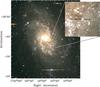 |
Fig. 1 RGB-image of M 33 and Var C. The colour image was generated from the R, V, and B band images from the Thüringer Landessternwarte (TLS) Tautenburg taken 6 January 2008. North is up and east to the left. |
LBVs have a high mass loss rate. During their quiet phase, this mass loss rate is of the order of 10-7–10-5M⊙/yr, while during their S Dor eruption phase, this can reach up to 10-5–10-4M⊙/yr (Humphreys & Davidson 1994).
By sweeping up the slower older stellar wind of earlier phases and S Dor cycles, as well as through mass ejections during a giant eruption, small (<5 pc, Weis 2011) circumstellar LBV nebulae are formed. These LBV nebulae contain CNO processed material from the star and are therefore rich in nitrogen and helium but low in oxygen and carbon (Maeder 1983).
To further determine the characteristics of LBVs it is necessary to find more of these stars. In Local Group galaxies, stars can be resolved spatially, and individual stellar parameters can be derived. The Local Group also provides different types of galaxies, hence different environments, and is therefore an ideal place to look for LBVs.
Periodicity on smaller timescales has already been known to occur in LBVs. The photometric variations in AG Car, an LBV in the Milky Way, where found by van Genderen (2001) to oscillate with periods of the order of one year (P0 = 371.4 d; P1 = 305 d or 475 d). Both periods appear superimposed. Shemmer et al. (2000) reported the M 33 candidate LBV UIT301 (also named B416) to show a periodicity of 8.26 days.
The periodicities found so far belong to the short S Dor variability (S-SD). Only a few indications for periodicities of the long S Dor type (L-SD) have been reported (van Genderen et al. 1997). A likely reason for it is that for most LBVs, the time baseline of the light curve is too short. Even if data from past centuries are available, these are often only a few data points so that the resulting light curve is quite patchy. A recently reported exception is the LMC LBV R71 (Walborn et al. 2014).
The Local Group spiral galaxy M 33 (classified as Scd) is located at a distance of approximately 840 kpc (distance modulus of 24.53±0.11 mag, Scowcroft et al. 2009). The proximity and low inclination of M 33 make it an excellent target for studying single stars. It also provides the possibility to study LBVs in an environment with a fairly low metallicity (Z = 0.008).
Hubble & Sandage (1953) first noticed the variability of several massive stars, which include Var C in M 33. Based on this publication, those stars were referred to as Hubble-Sandage variables. Finally together with the P Cyg- and S Dor-like variables, they were united under the term LBVs (Conti 1984).
With α2000 = 1:33:35.14 and δ2000 = 30:36:00.55, Var C is located only about 5′ south-west of the centre of M 33 (Fig. 1). Figure 2 shows the Hα-image (upper panel) and the continuum-subtracted Hα-image (lower panel) of Var C and its surroundings. After comparing both images, Var C shows a bright Hα emission, while neighbouring stars do not.
In the continuum-subtracted Hα-image, Var C seems to be surrounded by a faint ring-nebular-like structure with a radius of approximately 50 pc, which would be consistent with the star’s main sequence bubble. Weaver et al. (1977) give a radius of approximately 30 pc for the size of such a bubble, depending on the density of the surrounding interstellar medium (ISM).
Since both photometric and spectral observations of Var C have been made numerous times in the past, this provides us with the rare chance to trace the behaviour of an LBV over a wide span of time. For Var C we compiled a light curve that has a significant length (more than 100 years) in combination with a reasonable coverage of data points. This gives the chance not only to look for long time variations, but also to check whether these variations might be periodic. Since the origin of the variabilities in LBVs is not known yet, finding a periodic behaviour could give a hint of the underlying mechanism for these variations.
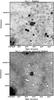 |
Fig. 2 Hα-image (upper panel) and continuum-subtracted Hα-image (Hα – R; lower panel) of Var C and its surroundings. Images were produced from NOAO LGGS data and have a size of about 150 pc × 150 pc. North is up and east is to the left. |
Log of observations.
2. Observations and data analysis
2.1. CCD imaging
2.1.1. Observations from TLS
Observations with the 2 m-telescope of the Thüringer Landessternwarte (TLS) Tautenburg in its Schmidt mode were taken during several runs between January 2006 and October 2011. The SITe detector was used with 2048 × 2048 pixels and an image scale of 1.̋23/pixel (FOV: 42′ × 42′) in combination with broadband Johnson B, V, R filters or a narrowband (100 Å) Hα filter, respectively. A standard data reduction (bias correction, flatfielding) was carried out using IRAF and a photometric analysis was performed using CCDCAP (Mighell 1998).
2.1.2. Observations from CAHA
We derived photometric data during our M 33 survey using the Calar Alto Faint Object Spectrograph (CAFOS) in its imaging mode at the 2.2 m-telescope at the Calar Alto Observatory (Centro Astronómico Hispano Alemán (CAHA)). The data were recorded from July to October 2006 during three runs in service mode using CAFOS at the 2.2 m-telescope. SITe-1d detector with 2048 × 2048 pixels, an image scale of 0.̋53/pixel and a field of view of about 16′ × 16′ was used. Images were taken in B and R filters. Basic data reduction was performed using IRAF. Subsequently, photometry was carried out using DOLPHOT (Dolphin 2000).
2.1.3. Observations from COoSAI
CCD observations at the Crimean Observatory of Sternberg Astronomical Institute (COoSAI) were made during 19 nights between October 2005 and October 2009. The 60 cm reflector (C60) equipped with an Apogee AP47 camera and a wide-field telescope (the 50 cm Maksutov camera-AZT-5) equipped with a Pictor camera were used. The typical uncertainty of our estimates is 0.1 mag (0.2−0.5 mag for stars fainter than 17 mag).
2.1.4. Observations from WIYN
Between August 2002 and July 2005, observations were made with the 3.5 m-telescope at the Wisconsin-Indiana-Yale-NOAO (WIYN) Observatory. The Mini-Mosaic imager consisting of two CCDs with 4096 × 2048 pixels, a field of view of 9′6 × 9′6, and an effective sampling of 0.̋28/pixel was used. A basic data reduction was performed using IRAF. PSF photometry was carried out using IRAF/DAOPHOT. A detailed description of the analysis method is given in Pellerin & Macri (2011).
2.1.5. Observations from the DIRECT project
Unpublished data from the DIRECT project taken between September 1996 and November 1998 were used to supplement the light curve. A description of the data and the analysis method can be found in Pellerin & Macri (2011). The DIRECT project (e.g. Kaluzny et al. 1998) was carried out to determine the direct distances to M 31 and M 33 using Cepheids and detached eclipsing binaries. CCD observations with 1-m class telescopes in BVI filters started in 1996.
2.1.6. Archival data from NOAO
Archival data from the National Optical Astronomy Observatory Local Group Galaxies Survey (NOAO LGGS; Massey et al. 2001) taken with the 4 m-telescope at Kitt Peak National Observatory (KPNO) in October 2000 and September 2001 were also used to perform photometric analysis. These images consisted of 8192 × 8192 pixels and had an image scale of 0.̋271/pixel (FOV: 36′ × 36′).
A basic data reduction (bias correction, flat fielding, etc.) was already done by Massey et al. (2002), but photometry was not yet available when we started our project. We therefore performed PSF photometry using IRAF/DAOPHOT. The comparison with Massey et al. (2006) revealed only a small photometric offset of a tenth of a magnitude, which was corrected.
2.2. Photographic plate scans from TLS
Our photometric data set was supplemented by archival photographic plates of M 33 taken between August 1963 and December 1996 with the Tautenburg Schmidt telescope (free aperture 1.34 m, focal length 4 m). A single Tautenburg plate covers an unvignetted field of  with a plate scale of
  per mm. We made use of 77 B plates, all of which had been digitised with the Tautenburg Plate Scanner (Brunzendorf & Meusinger 1999). The digital images have a pixel size of
  .
.
Data was reduced in an analogous way to the method applied by Henze et al. (2008) for analysing digitised photographic plates of M 31 taken with the same telescope. We used the Source Extractor package (Bertin & Arnouts 1996) for object detection, background correction, and relative photometry. The photometric calibration was done using the M 33 part of the Local Group Galaxies Survey (LGGS, Massey et al. 2006). A detailed description of the analysis method is given in Henze et al. (2008).
2.3. Heidelberg Digitized Astronomical Plates
We used the Heidelberg Digitized Astronomical Plates (HDAP) to obtain additional datapoints for the sparsely sampled era at the beginning of the 20th century. Twelve photographic plates of M 33 were taken with the 72 cm Walz-Reflector between 1908 and 1922. No detailed or specific information on the spectral sensitivity of the emulsions that were used could be derived from the observers’ notebook, except for one case (“blue sensitive”). We therefore treated all plates as blue-sensitive “normal” plates and calibrated the magnitudes into B band. We measured the brightness of Var C to fill the sparsely populated light curve for those epochs. The large spread in the quality of the plates prevented a consistent linearisation for this dataset. Therefore, magnitudes were derived using the classical Argelander method (Nijland 1901).
2.4. Historical data taken from literature
To trace the behaviour of Var C in the past, a light curve was created using data from both the literature and the archive. Since the historical data were either photographic magnitudes (mpg) or B magnitudes, we compiled a light curve in B. We calculated mpg into Johnson B magnitudes using the following conversion given in Meusinger et al. (2010): 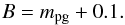 (1)B magnitudes were calculated for data points taken from Hubble & Sandage (1953), Sharov (1973), Rosino & Bianchini (1973), Lovas & Zsoldos (1988), and Sharov (1990).
In case no tabulated data existed, mpg data points were extracted from given light curves using DEXTER (Demleitner et al. 2001). Errors in time and magnitude are mainly due to uncertainties from extracting the data. A maximum error was assumed to be half the size of the data point symbol in the light curve plot. This gave an error of JD±36 days and mpg ± 0.051 mag for data values taken from Hubble & Sandage (1953), JD±18 days and mpg ± 0.023 mag for values from Rosino & Bianchini (1973), and JD±220 days and B ± 0.094 mag for values from Zharova & Sholukhova (2004).
Magnitudes derived from photographic plates or photometers already given in B magnitudes were taken from van den Bergh et al. (1975), Humphreys (1978), Humphreys & Warner (1978), Humphreys et al. (1984, 1988), and Kurtev et al. (1999). Further B CCD-photometry values came from Wilson (1991), Massey et al. (1995), Szeifert et al. (1996), Mochejska et al. (2001), Viotti et al. (2006), Humphreys et al. (2013b), and Valeev et al. (2013).
All B data values are collected in Tables 3 and 4.
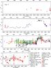 |
Fig. 3 B light curve of Var C between 1899 and 2013. For reasons of clarity and readability error bars are only given for data with uncertainties of more than 0.4 mag. The data values are listed in Tables 3 and 4. |
Additional V band data used in Fig. 8 are from Spiller (1992), Macri et al. (2001), and Shporer & Mazeh (2006).
For completeness, in the following we list published values for Var C, which had no observation times given. Therefore, these values could not be included in the light curves. The catalogue from Ivanov et al. (1993) lists Var C as star IFM_B 600. Values of V = 15.20 mag, B − V = 0.30 mag (B = 15.50 mag), and U − B = −0.40 mag (U = 15.10 mag) are given. Var C is listed as v267 by Fabrika & Sholukhova (1995) with values of V = 16.70 mag and B − V = 0.30 mag (B = 17.00 mag).
2.5. Spectral observations from SAO RAS
Two spectra were taken on 13 November 2004 and 22 October 2008 with the 6 m-telescope at the Special Astrophysical Observatory of the Russian Academy of Sciences (SAO RAS). The Multi-Pupil Fiber Spectrograph (MPFS; Sholukhova et al. 2007) and the Spectral Camera with Optical Reducer for Photometrical and Interferometrical Observations (SCORPIO; Afanasiev & Moiseev 2005) were used respectively.
3. Light curve of Var C
A light curve of Var C between 1899 and 2013 containing values from the literature, photometry done on archival data, and our observations is presented in Fig. 3. The corresponding data values are listed in Tables 3 and 4.
The earliest four data points found in the literature spread over almost 20 years and vary over one magnitude. Low data coverage during that time prevented us from reconstructing the stars photometric behaviour on short timescales. The overall trend indicates a peak around 1905 and, in total, a decline until 1915.
Additional plate data from HDAP (Fig. 3; filled red diamonds) further confirm the indication from the Mount Wilson data (Hubble & Sandage 1953; black dots) of a broad maximum between 1900 and 1915. The lack of data around 1905 and before 1899 prevents us from putting stronger constrains on the maximum.
More regular time coverage of Var C is available starting in 1918 when the star showed a brightness of approximately 17.5 mag in B consistently in the Mount Wilson and HADP data. Until the mid 1930s, the star remained at almost constant luminosity apart from some smaller variations of less than half a magnitude. Subsequently, the luminosity of Var C started to increase over more than ten years until it reached its first established prominent maximum. With a gap in the data coverage present between 1941 and 1945, the slope of the light curve towards the maximum is not sampled very well. This maximum around 1947 with a maximum brightness in B of about 15.4 mag lasted at least three years. The luminosity started to decline around 1950. The sparse data coverage also makes it hard to determine the minimum value with good accuracy, which is probably almost as faint as before rising.
Minor increases of up to one magnitude are seen around 1957 and 1963. Especially the later rise and decrease is very narrow with almost one magnitude in less than one month. A broader and less luminous minor maximum around 1967 can be assumed.
With the exception of smaller variations between 1970 and 1982, Var C stayed constant at a B brightness of ≈17 mag. Since most of the values at this phase are photographic or photoelectric measurements, there might be a zeropoint or colourterm offset. When taking this into account, it is probably more significant for judging the variability to only look at variations within each set of data values separately. Since all data of one data set were very likely processed in the same way, variations in the data values can be trusted to be real.
The next prominent maximum occurred around 1986 where the luminosity again rose to about 15.4 mag for about four years. The rapid rise – in particular in the R band (compare Fig. 1 from Humphreys et al. 1988) – was followed by a steep decline in luminosity, which occurred at the end of 1986. It can be seen well in the TLS plate data (Fig. 3, red crosses) but is also present in the data by Humphreys et al. (1988; Fig. 3, blue diamonds) and Massey et al. (1995; Fig. 3, yellow four-ray star). Within 120 days, variations of about one magnitude are seen.
Around 1990 the luminosity in B of Var C was almost back to a value before the rise. During the next 20 years minor and/or steeper increases and declines took place, namely in 1992, 1996, end of 2002, and 2007. The maximum around 2002/2003 was nearly as bright as the two previous prominent maxima, but a much steeper increase and a decrease is present in this one.
In September 2009 the luminosity in B was 17.56 mag. It brightened in October 2011 and reached a new maximum value of 15.87 mag on 1 September 2013 (Humphreys et al. 2013b) and has stayed at this new maximum light level ever since. That Var C stayed at maximum light during this time and did not pass through two close and short maxima, is even more evident in the V light curve, that has additional measurements (see Fig. 8, middle panel).
4. Spectra of Var C
The first spectra of Var C have already been reported in Hubble & Sandage (1953). Spectra were taken between November 1946 and November 1951. The first two spectra were taken in November 1946 and in August 1947, when Var C was in a phase of maximum light (see Fig. 3). The spectra show Ca ii K (λ3933) and Ca ii H (λ3968) in absorption. Both lines have nearly equal strengths. According to Hubble & Sandage (1953), this is “[...] indicating that the spectral class is at least later than F0”. In the first of these two spectra, Hγ and Hδ are weakly present in absorption, while the second one shows no hydrogen lines. The next spectra were taken during descending light. In 1949 the spectra showed faint Hβ emission but no Ca ii K or Ca ii H lines were visible. The spectra taken from August to October 1951 show a much stronger Hβ line and an Hγ line, both in emission. Ca ii K and Ca ii H were seen in absorption. In November 1951, Hβ and Hγ were still seen in emission, but no Ca ii K and Ca ii H lines were visible.
Based on their spectrum obtained in September 1973, Sharov et al. (1975) reported that Var C was displaying a bright Hα emission. Humphreys (1975) recorded two spectra taken in October and November 1974 that showed several hydrogen, He i Fe ii, and [Fe ii] lines in emission, as well as Ca ii K in absorption. She stated that Var C is an η Carina-like object.
Humphreys (1978) compared a spectrum taken two years later in August 1976 with the two spectra taken previously. The hydrogen and He i emission lines had become weaker and some of the Fe ii and [Fe ii] lines were no longer seen.
The spectra taken in November 1983 by Kenyon & Gallagher (1985) showed Hα, Hγ, and numerous Fe ii lines in emission. All these lines showed pronounced P-Cygni profiles. Strong Mg iiλ4481 was seen in absorption. Kenyon & Gallagher (1985) suggested a temperature for Var C at that time of only slightly less than <10 000 K.
Several optical spectra of Var C taken between November 1985 and September 1987, as well as one UV spectrum (August 1986), were presented in Humphreys et al. (1988). The spectra of Var C taken in 1985 – corresponding to a maximum phase of Var C – showed only Hα and Hβ in emission. Several strong lines of ionised metals including Fe ii were seen in absorption. Humphreys et al. (1988) stated that the spectrum resembles that of an early F-type supergiant (F0Ia–F5Ia). They estimated a surface temperature of ≈7500 K. The optical spectra taken in 1986 showed weaker metallic lines, indicating – together with its ratio of the Ca ii K and Ca ii H lines – a higher surface temperature of up to 9000 K and a spectral type of about A2 to A3 (Humphreys et al. 1988).
The UV spectrum showed no emission lines, but Fe ii lines in absorption underlined the estimation of Var C being an A-type star at that time. In the high-resolution spectra taken in September 1987 Fe ii and other metallic lines were seen in absorption, as well as several Fe ii-lines in emission. Hα, Hβ, and Hγ showed P-Cygni profiles.
Szeifert et al. (1996) presented optical spectra taken in November 1991, October 1992, and December 1992. An additional UV spectrum was taken in July 1992. The 1992 spectra were described to show weak He i lines in absorption corresponding to a temperature >10 000 K at that time. A comparison made between the spectra from 1987 (presented in Humphreys et al. 1988), 1991, and 1992 shows that the hydrogen and Fe ii emission lines were getting stronger. Both optical and UV spectra were described to be consistent with a post-maximum phase of Var C.
A spectrum taken in December 1993 (Massey et al. 1995, 1996, 2007) showed pronounced hydrogen lines in emission and several Fe ii and [Fe ii] in emission. He i is weakly seen. Spectra taken in December 2004 and January 2005 by Viotti et al. (2006) showed strong hydrogen lines in emission. Several Fe ii and [Fe ii] lines were seen in emission. A spectral type of B[e] was given.
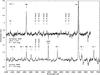 |
Fig. 4 SAO RAS spectra of Var C taken on 13 November 2004 (upper spectrum) and 22 October 2008 (lower spectrum). |
Clark et al. (2012) reported on two spectra taken on 30 November 2003 and 29 September through 2 October 2010. The first one showed Hβ in emission and numerous metallic absorption lines. The spectrum was compared to a spectrum of the F0-F5Ia+ hypergiant B324. The spectrum taken in 2010 showed Hα, Hβ, and Hγ in emission. Several He i lines were also seen in emission, as was Fe ii. The emission lines showed P-Cygni profiles. Var C became hotter from 2003 to 2010. As seen from the light curve, the luminosity of Var C decreased during this time.
Two SAO RAS spectra taken on 13 November 2004 and 22 October 2008 are presented in Fig. 4. The spectrum recorded in November 2004 shows Hα, Hβ, and Hγ in emission. Several weak Fe ii lines are present in emission. In the spectrum from October 2008, Hα and Hβ are seen in emission. Several He i and some Fe ii lines are very present in emission. Comparing this development with the slope of the light curve shows that Var C faded between the end of 2004 and the end of 2008 of about 0.7 mag. This is consistent with the spectra and indicates that the star is entering a hot phase.
A spectrum of Var C taken 3 October 2010 (Humphreys et al. 2014) shows Balmer lines in emission. Several He i and numerous Fe ii and [Fe ii] lines are also seen in emission. Pronounced P-Cygni profiles are present in the spectrum. With respect to the light curve, the spectrum was taken after a minimum, with Var C increasing its luminosity, but still representing a hot star.
A low-resolution spectrum taken on 18 September 2013 by Viotti et al. (2013) is described to show hydrogen lines in emission.
Two spectra taken on 5 October 2013 and 1−2 November 2013 were reported by Valeev et al. (2013). The spectra were described to show Fe ii lines in emission, as well as [Fe ii] and strong hydrogen lines. He i was seen very weakly in absorption. P-Cygni profiles were present in the hydrogen lines and the majority of the Fe ii lines.
Another spectrum taken on 7 October 2013 by Humphreys et al. (2014) showed much weaker hydrogen lines in emission, Ca ii and Mg ii in absorption, and Fe ii in emission with P-Cygni profiles. The spectrum is classified as late A-type. This spectral type was still confirmed with an LBT IR spectrum taken January 2014.
Table 2 summarises the optical spectral observations of Var C. The spectrum reported by Burggraf et al. (2011) taken in September 2007 was not that of Var C, but of a different star1. Where not already given in the literature, a spectral type has been estimated based upon the description of the spectrum in the literature. The criteria for classifications were derived from spectral descriptions given by Jaschek & Jaschek (1987).
5. Discussion
5.1. Periodicity
While several semi-periodic structures are known to exist in the light curves of LBVs on timescales of about ten years, the periods are less stable than in Cepheids (van Genderen 2001), for example. The extremely long light curve of Var C that we established manifests an excellent unique data set to make a reliable analysis for even long-term trends and periods. A first inspection of the light curve of Var C reveals two pronounced maxima. The first maximum occurred around 1947 and a second one around 1986. To investigate the long scale variability in B of Var C, we analysed the periodicity using a Fourier analysis performed with Period04 (Lenz & Breger 2005). Data values from van den Bergh et al. (1975) were excluded because of the relatively large magnitude uncertainties of 0.7 mag, as was one data point from WIYN for the same reason. The B data values were averaged by month in order to avoid being sensitive to small scale variations (below a month). A light curve of these averaged data is presented in Fig. 7 (upper panel).
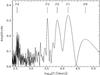 |
Fig. 5 Power spectrum derived from the B magnitude values presented in the upper panel of Fig. 7. The highest peak (P1) corresponds to a period of 42.3 years. The values for the other peaks are given in Table 5. |
Figure 5 shows the power spectrum derived from the B data values. A bright peak is seen at P1 = 15 440 days = 42.3 years. Two more peaks are present at P2 = 6926 days = 19.0 years and P3 = 3356 days = 9.2 years. The peaks around P4 corresponding to a period of approximately one year are most probably due to the sampling of the data. The very broad and low amplitude peak (P0) with the highest period is due to the apparent overall increase in the luminosity. Such a secular trend of brightening is also seen in the light curve of other LBVs like η Car. Table 5 lists the parameters of the main peaks labelled in Fig. 5.
As seen from Table 5 periods, P1 and P2 are roughly multiples of period P3. The amplitudes of P1, P2, and P3 are also in the same order of magnitude. This could mean that the 40-year period is not real, which would then favour the twenty- or ten-year period.
To gain a better understanding of the structures found in the power spectrum, synthetic light curves were produced. Therefore, synthetic data modelling the main features of Var C’s light curve were generated. Subsequently, Period04 was used on these data.
One of these synthetic light curves was generated with one data point per month at only six months per year, while no data points were set the other half of the year. This was done to reproduce that M 33 is only observable during roughly half a year each year from the northern hemisphere. Using this setup, we were able to reproduce the broad bump consisting of several peaks around P4. When adding data points for the other six months, this peaks vanish. This indicates that the peak around P4 is indeed produced by the sampling of the data.
As another test, data points were added to the light curve of Var C by averaging neighbouring data points and adding the averaged value as a new data point in between them. This method was applied twice, so that a light curve with two times and another with four times the original number of data points were created. Both times Period04 found the same peaks (P1, P2, P3) with P1 having the highest amplitude, even though this still does not necessarily mean that the 40-year period is real.
The phase diagram corresponding to the maximum peak at a frequency of ν = 6.477 × 10⁻⁵ per day (corresponding to period P1 = 15 440 days = 42.3 years) is given in Fig. 6. The data has been binned into eight bins and these binned data has been fitted with an akima spline. A zero point offset in time of 3000 days was applied.
At least one prominent maximum is seen in the phase diagram. A second, smaller maximum at approximately half of the period might be assumed, but data scattering is much larger and renders it quite uncertain. This minor maximum is represented in Fig. 5 by peak P1. It still might be that the period is only approximately 18−20 years with the maximum amplitude not always equally strong. Another interpretation would be that the period is ≈40 years with a major maximum and a minor maximum. Assuming the last major maximum was around 1986, the next strong maximum phase of Var C should occur around 2028±3. Nevertheless, (semi-)periodic behaviour on large time scales is seen in the light curve.
Some uncertainties arise from the fact that the data are from various telescopes and that transformations had to be made between different magnitude systems (mpg, B). Assuming all data of one dataset have been processed in the same way, variations within such a dataset are more significant and give information about variability on smaller scales.
van Genderen (2001) found two frequencies (both roughly a year; P0 = 371.4 days; P1 = 305 days or 475 days) present in AG Car and superimposed on each other, resulting in a beat cycle of about 20 years. This looks similar to the 20-year period found in Var C’s light curve (if assuming maxima of different amplitudes).
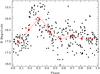 |
Fig. 6 Phase diagram using a frequency of ν = 6.477 × 10⁻⁵ 1/d (P1 ≈ 42.3 years). The data has been binned (red dots) and the binned data fitted with an akima spline (red line). A zero point offset in time of 3000 days was applied. |
To check whether the periodicity in Var C’s light curve on this long time scale might only be the result of a superposition of periodicities on smaller timescales, we also looked at the small variations of Var C. For this we used the data from the TLS plate scans to have a consistent data set. In addition we also used V band data from Macri et al. (2001; images taken between September 1996 and October 1997) and Shporer & Mazeh (2006; images taken between September 2000 and November 2003), covering a range of six years to search for periodicity.
Even though variabilities on smaller scales are obviously present in the light curve of Var C, no clear period around a year was found. Such small and intermediate scale periodicities are not even seen when looking only at separate datasets and at datasets with the highest data coverage. This means either that the data coverage is still not good enough to find these small scale periodicities or that the long-term periodicity found in Var C is not just a beat cycle resulting from the superposition of two or more frequencies, as in AG Car. This could mean that the periodicity of Var C is caused by a different mechanism than the long-term periodicity of AG Car.
Also no periodicity of days was found in Var C’s light curve as in UIT301. Shemmer et al. (2000) reported the M 33 LBV UIT301 (also named B416) to show a periodicity of 8.26 days. Even though Sholukhova et al. (2004) stated that this is the half of the orbital period and therefore light variations are due to a close interacting binary rather than to intrinsic variability in luminosity.
With an amplitude of approximately 1.5−2 mag for the major peak (and 0.5 mag for a minor peak – if present) and with an assumed length of 42 years, Var C can be classified as a strong-active S Dor member with a long S Dor (L-SD) cycle, as defined by van Genderen (2001). Comparing Var C’s light curve with the light curves of other strong-active S Dor members given in van Genderen (2001), it is seen that, induced by sparse data coverage, the light curves are quite patchy. Time approximations for the L-SD durations indicate variabilities of decades, but no periodicity on these timescales can obviously be seen from the light curves. Most light curves show secular trends of de- or increasing light (e.g. R110). Some light curves show a single maximum (e.g. R116).
So far, regular–periodic–variations have not been known to be a common feature of LBVs. With the really long-term light curves, which have come up more recently, the first cases are being observed right now. Walborn et al. (2014) have reported on the LMC LBV R71 to show periodic variability on a timescale of about 40 years. More recently, the maxima have appeared more frequently and with a larger amplitude. This is similar to what was observed for the LBV Var B in M 33 between 1930 and 1950, when Hubble & Sandage (1953) found three maxima with steadily increasing amplitudes.
Periodicity on a timescale of several decades is unusually long. Common mechanisms causing periodic light variations, such as the κ-mechanism, occur on much smaller timescales (days up to a few months). So far, no intrinsic stellar mechanism has been known to cause such long-term periodicity.
Recently, Koenigsberger et al. (2010) have found a 40-year cyclic variation in HD 5980, which is a multiple system consisting of a close binary (two Wolf-Rayet type stars orbiting each other with a period of 19.3 days) and a third O-type star component. The authors suggest that the observed slow variations due to changes in the radius were superimposed by strong and short-duration eruptions caused by the binary companion.
The similarity in the length of the periods found in Var C and HD 5980 might lead to the question of whether periodicity caused by interaction in a binary system is a general phenomenon and thus whether Var C might also consist of more than one component. So far, no hints of binarity have been reported for Var C. Also the available high-resolution spectra do not show evidence of any binarity.
Nevertheless, the photometric variations seen in HD 5980 and Var C appear to be quite different. The light curve of HD 5980 (see Koenigsberger et al. 2010 Fig. 1) shows a sudden, short eruption after a slow brightening over several years. This peak is very steep and narrow. In contrast to that, Var C’s first maximum shows a relatively slow rise and fall. The second maximum appears slightly steeper and narrower than the first one, but is still much broader than the peak seen in HD 5980. Both of Var C’s maxima last at least a few years.
If Var C is indeed a single star, the similarity of the period might just be coincidental. In that case a completely different underlying mechanism has to be responsible for the (semi-)periodicity of Var C.
5.2. Temperature variations
By converting the photometrical colours of Var C into temperatures, a more physical interpretation can be made. For this we used Eqs. (4b) through (4e) from Parker & Garmany (1993; see also references within).
For (B − V)0< 0.0 we used Eq. (4b):  (2)for 0.0 ≤ (B − V)0< 0.2 Eq. (4c) was applied:
  (3)For 0.2 ≤ (B − V)0< 0.5 Eq. (4d) was used,
  (4)and for 0.5 ≤ (B − V)0 Eq. (4e) was applied:
  (5)Parker & Garmany (1993) used these equations to calculate Teff for stars with only photometric values available, hence for stars without any further spectral classification. According to them, Eq. (2) is not valid for supergiants. Supergiants would be cooler (a few 1000 K, depending on the spectral type) than dwarfs of the same spectral type. Therefore, the estimated temperature would be to high, if the star was a supergiant.
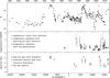 |
Fig. 7 B light curve of Var C (upper panel). In comparison to Fig. 3, the B values here have been averaged by month. The corresponding temperatures and spectral types are given in the middle and lower panels, respectively. |
Furthermore, the calculation of the temperature strongly depends on the assumed reddening of the star. Therefore, we determined the reddening from an U − B versus B − V colour–colour diagram using stars in the surrounding of Var C. Since Var C only has a few neighbouring stars, the determination of reddening is rendered somewhat uncertain. A mean value of 0.17±0.07 was found. This is in good agreement with a reddening value for Var C from e.g. Viotti et al. (2006), who used AV = 0.6, which equals E(B − V) = 0.19. We calculated temperatures for three different values of E(B − V) of 0.10, 0.17, and 0.24.
Because of these uncertainties (validity of equations, reddening), these temperature calculations can only give a rough estimate. Nevertheless, they can be used to trace the general development of Var C’s temperature curve. Table 6 lists the calculated temperatures. The calculations were done for colours derived from own photometries and from photometries from the literature. The resulting temperature curve is given in Fig. 7 (middle panel).
Figure 7 illustrates the connection between light variations and changes in temperature, hence in spectral type. The upper panel shows the B light curve of Var C. In contrast to the light curve presented in Fig. 3, the B values here were averaged by month. These are also the B values used for analysing the periodicity. The middle panel presents the corresponding temperatures. Literature values and temperature estimated from photometric values are plotted. Finally, the lower panel shows the spectral types of Var C at different times. Values are either taken directly from the literature or are estimated spectral types from the description of a spectrum in the literature (see also Table 2).
Even though the coverage with spectral data is quite patchy, it is seen that during maximum light, the star resembles an A- or F-type star. During phases of minimum light an O- or B-type star is seen. Since changes in the spectral type are caused by changes in the temperature, this trend is also seen in the temperature curve. For example, during the maximum around 1986, temperatures around 10 000 K are seen, while temperatures above 16 000 K are present just before this maximum. Also the decrease in luminosity between 2003 and 2010 is accompanied by a rise in the temperature curve, while lower temperatures are measured again in the beginning maximum after 2010.
Some additional V band data were available for Var C. Therefore, a V light curve is also presented in the middle panel of Fig. 8. For a comparison, the B light curve is shown in the upper panel of the same figure. The corresponding B − V colour curve is given in the lower panel.
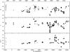 |
Fig. 8 B and V light curves and B − V colour curve of Var C. Crosses: TLS plate data; filled upwards triangles: DIRECT; stars: NOAO; filled downwards triangles: WIYN; stars with six rays: TLS CCD data; filled squares: COoSAI; filled diamonds: Humphreys (1978), Humphreys & Warner (1978), Humphreys et al. (1984, 1988); open four-ray stars: Massey et al. (1995); open circles: Wilson (1991); filled circle: Spiller (1992); open squares: Szeifert et al. (1996); open upwards triangles: Macri et al. (2001); open diamonds: Mochejska et al. (2001); plus signs: Shporer & Mazeh (2006); filled five-ray stars: Viotti et al. (2006); filled small dots: Viotti et al. (2013); open small dot: Roberto Viotti, Franco Montagni (priv. comm.); open five-ray stars: John Martin (priv. comm.); filled four-ray stars: Humphreys et al. (2013b); and open downwards triangles: Valeev et al. (2013). Only data sets containing V band data were used in these plots. Only errors larger than 0.3 mag are shown. |
As for changes in the spectral type, changes in the colour (here B − V) also represent changes in the temperatures of a star. Larger B − V values indicate redder, hence cooler stars. As seen from Fig. 8, the B − V colour curve also shows that Var C is redder and cooler when it is in maximum light.
All these described trends in the temperature and light variations – cooler when in minimum light and hotter while in maximum light – indicate S-Dor behaviour, the variability intrinsic to LBVs. A detailed SED fitting, however, is not possible because for most epochs, no multi-wavelength observations have been recorded.
6. Conclusions
We investigated the long-term photometric and spectral behaviour of the LBV Var C in M 33. We classified Var C as a strong-active S Dor member with a long S Dor (L-SD) cycle. A long-term (semi-)periodicity with a period of 42.3 years is detected with the chance of the real period being 19.0 years or even 9.2 years. If a long-term periodicity of approximately 42 years is present in the B light curve of Var C, the next maximum light should occur around 2028±3. However, developments since 2010 have shown that Var C is already entering a phase of maximum light 15 years earlier, which is not consistent with the longest possible period, but is within the uncertainty that matching both the shorter periods.
Var C has been in maximum light for more than one year now (Humphreys et al. 2013b). Even though Var C is approximately 0.5 mag fainter than during the two prominent maxima in 1947 and 1986, the slope of the rise and the duration so far fits the previous two bright maxima, indicating a comparable eruptive state. Var C’s spectral, colour, and temperature curves, together with its corresponding light curves, show variations that indicate an S Dor variability.
Several measurements were reported during the tracing of the current changes in the light curve of Var C. This shows that even though Var C is a long known LBV, it is still necessary and important to trace its behaviour further in order to fully understand the various features of LBVs.
As recently shown for the LBV R71 in the LMC (Walborn et al. 2014), only by compiling a light curve over ~100 years is it possible to detect photometric variation on long timescales. These features’ (as in the case of R71) two broad maxima at 1914 and 1939 give rise to physical events in the star, which are currently unknown and far from being understood. The brightness of R71 has increased during the last five years and reached the highest maximum ever reported (Walborn et al. 2014). In addition, the R71 photometric behaviour seems like what we found for Var C. Indications of regular change between bright and dim peaks with similar maxima and minima (in magnitudes) are visible in R71, as for Var C. R71 shows broad and overlayed narrow maxima that appear to have some (but not necessarily strict) periodicity, similar to the structures in the light curve of Var C that we report in this paper. Also, an overlayed secular trend towards higher luminosity seems to be present, again very similar to the one in Var C.
Another feature of the R71 light curve is the trend toward the duration of the maxima being shorter with increasing amplitudes (Walborn et al. 2014). This may also be present in the light curve of Var C. It also may explain the rather small amplitude of the 1905 maximum of Var C indicated in our light curve. The increasing time interval between outbursts of R71 (Walborn et al. 2014) does not appear to be present in the light curve of Var C. Therefore, Var C may not (yet) be in an evolutionary phase of accelerated changes (e.g. Moriya et al. 2014). This is also supported by the absence of Ca ii emission lines (and therefore a dense envelope), as reported for R71 (Bonanos et al. 2009; Gamen et al. 2012; Mehner et al. 2013). The historic light curve of R71 appears to be rather more strongly modulated than that of Var C, and especially the recent outburst of R71 (Gamen et al. 2012; Mehner et al. 2013) is much more extreme than the one of Var C (Humphreys et al. 2013a).
Based on the similarity to R71, one may speculate that the semi-periodicity plus the secular brightening trend in the light curve of Var C is an indication that the evolutionary state of both stars is going to change, and the current, rather unexpected brightening of Var C is an indication of a coming large eruption as in R71. If this should happen to Var C soon, it would give rise to a new phenomenon in LBVs: large eruptions following L-S Dor variability are overlayed on a secular brightening trend on timescales of 100 years and may be linked to accelerated evolution towards a supernova. A monitoring of the subsequent development of the current bright state of Var C is therefore much needed. Clearly, a hunt for more historic plates will be very fruitful.
Online material
Summary of optical spectra of Var C.
Light curve data from the literature.
Light curve data.
Based on a misidentification during service.
Acknowledgments
We thank Marko Röder and Bringfried Stecklum for service observations with the 2 m-Alfred-Jensch-telescope of the Thüringer Landessternwarte (TLS) Tautenburg. Thanks go to Otmar Stahl for helpful comments on the classification of our spectrum of Var C and Gloria Koenigsberger for discussions on the variability of massive stars. We thank Roberta M. Humphreys and Kris Davidson for inspiring discussions and helpful comments. Special thanks go to Roberta M. Humphreys for her help with line identification. We are grateful to Artie P. Hatzes, John Martin, and René Hudic for comments and Chris Evans for a spectrum of Var C. B. Burggraf is thankful for support by a stipend from the “Wilhelm and Günter Esser foundation”. O. Sholukhova and A. Zharova are grateful for RFBR grant No. 13-02-00885, the grant “Leading Scientific Schools of Russia”, and grant No. 14-50-00043 of the Russian Scientific Foundation. This work made use of the HDAP which was produced at the Landessternwarte Heidelberg-Königstuhl under grant No. 00.071.2005 of the Klaus-Tschira-Foundation. We thank the referee for detailed comments.
References
- Afanasiev, V. L., & Moiseev, A. V. 2005, Astron. Lett., 31, 194 [NASA ADS] [CrossRef] [Google Scholar]
- Bertin, E., & Arnouts, S. 1996, A&AS, 117, 393 [NASA ADS] [CrossRef] [EDP Sciences] [Google Scholar]
- Bonanos, A. Z., Massa, D. L., Sewilo, M., et al. 2009, AJ, 138, 1003 [NASA ADS] [CrossRef] [Google Scholar]
- Brunzendorf, J., & Meusinger, H. 1999, A&AS, 139, 141 [NASA ADS] [CrossRef] [EDP Sciences] [Google Scholar]
- Burggraf, B., Weis, K., Bomans, D. J., & Henze, M. 2011, Bull. Soc. Roy. Sci. Liège, 80, 356 [NASA ADS] [Google Scholar]
- Clark, J. S., Castro, N., Garcia, M., et al. 2012, A&A, 541, A146 [NASA ADS] [CrossRef] [EDP Sciences] [Google Scholar]
- Conti, P. S. 1984, in Observational Tests of the Stellar Evolution Theory, eds. A. Maeder, & A. Renzini, IAU Symp., 105, 233 [Google Scholar]
- Demleitner, M., Accomazzi, A., Eichhorn, G., et al. 2001, in Astronomical Data Analysis Software and Systems X, eds. F. R. Harnden, Jr., F. A. Primini, & H. E. Payne, ASP Conf. Ser., 238, 321 [Google Scholar]
- Dolphin, A. E. 2000, PASP, 112, 1383 [NASA ADS] [CrossRef] [Google Scholar]
- Fabrika, S., & Sholukhova, O. 1995, Ap&SS, 226, 229 [NASA ADS] [CrossRef] [Google Scholar]
- Gamen, R., Walborn, N., Morrell, N., Barba, R., & Fernandez Lajus, E. 2012, Central Bureau Electronic Telegrams, 3192, 1 [NASA ADS] [Google Scholar]
- Henze, M., Meusinger, H., & Pietsch, W. 2008, A&A, 477, 67 [NASA ADS] [CrossRef] [EDP Sciences] [Google Scholar]
- Hubble, E., & Sandage, A. 1953, ApJ, 118, 353 [NASA ADS] [CrossRef] [Google Scholar]
- Humphreys, R. M. 1975, ApJ, 200, 426 [NASA ADS] [CrossRef] [Google Scholar]
- Humphreys, R. M. 1978, ApJ, 219, 445 [NASA ADS] [CrossRef] [Google Scholar]
- Humphreys, R. M., & Davidson, K. 1994, PASP, 106, 1025 [NASA ADS] [CrossRef] [Google Scholar]
- Humphreys, R. M., & Warner, J. W. 1978, ApJ, 221, L73 [NASA ADS] [CrossRef] [Google Scholar]
- Humphreys, R. M., Blaha, C., D’Odorico, S., Gull, T. R., & Benvenuti, P. 1984, ApJ, 278, 124 [NASA ADS] [CrossRef] [Google Scholar]
- Humphreys, R. M., Leitherer, C., Stahl, O., Wolf, B., & Zickgraf, F.-J. 1988, A&A, 203, 306 [NASA ADS] [Google Scholar]
- Humphreys, R. M., Davidson, K., Grammer, S., et al. 2013a, ApJ, 773, 46 [NASA ADS] [CrossRef] [Google Scholar]
- Humphreys, R. M., Weis, K., Burggraf, B., et al. 2013b, ATel, 5362, 1 [NASA ADS] [Google Scholar]
- Humphreys, R. M., Davidson, K., Gordon, M. S., et al. 2014, ApJ, 782, L21 [NASA ADS] [CrossRef] [Google Scholar]
- Ivanov, G. R., Freedman, W. L., & Madore, B. F. 1993, ApJS, 89, 85 [NASA ADS] [CrossRef] [Google Scholar]
- Jaschek, C., & Jaschek, M. 1987, Sky and Telescope, 74, 612 [NASA ADS] [Google Scholar]
- Kaluzny, J., Stanek, K. Z., Krockenberger, M., et al. 1998, AJ, 115, 1016 [NASA ADS] [CrossRef] [Google Scholar]
- Kenyon, S. J., & Gallagher, III, J. S. 1985, ApJ, 290, 542 [NASA ADS] [CrossRef] [Google Scholar]
- Koenigsberger, G., Georgiev, L., Hillier, D. J., et al. 2010, AJ, 139, 2600 [NASA ADS] [CrossRef] [Google Scholar]
- Kurtev, R. G., Corral, L. J., & Georgiev, L. 1999, A&A, 349, 796 [NASA ADS] [Google Scholar]
- Lenz, P., & Breger, M. 2005, Commun. Asteroseismol., 146, 53 [NASA ADS] [CrossRef] [Google Scholar]
- Lovas, M., & Zsoldos, E. 1988, IBVS, 3193, 1 [NASA ADS] [Google Scholar]
- Macri, L. M., Stanek, K. Z., Sasselov, D. D., Krockenberger, M., & Kaluzny, J. 2001, AJ, 121, 870 [NASA ADS] [CrossRef] [Google Scholar]
- Maeder, A. 1983, A&A, 120, 113 [NASA ADS] [Google Scholar]
- Massey, P., Armandroff, T. E., Pyke, R., Patel, K., & Wilson, C. D. 1995, AJ, 110, 2715 [NASA ADS] [CrossRef] [Google Scholar]
- Massey, P., Bianchi, L., Hutchings, J. B., & Stecher, T. P. 1996, ApJ, 469, 629 [Google Scholar]
- Massey, P., Hodge, P. W., Holmes, S., et al. 2001, BAAS, 33, 1496 [NASA ADS] [Google Scholar]
- Massey, P., Hodge, P. W., Holmes, S., et al. 2002, BAAS, 34, 1272 [NASA ADS] [Google Scholar]
- Massey, P., McNeill, R. T., Olsen, K. A. G., et al. 2007, AJ, 134, 2474 [NASA ADS] [CrossRef] [Google Scholar]
- Massey, P., Olsen, K. A. G., Hodge, P. W., et al. 2006, AJ, 131, 2478 [NASA ADS] [CrossRef] [Google Scholar]
- Mehner, A., Baade, D., Rivinius, T., et al. 2013, in Massive Stars: From alpha to Omega, Conf., 168 [Google Scholar]
- Meusinger, H., Henze, M., Birkle, K., et al. 2010, A&A, 512, A1 [NASA ADS] [CrossRef] [EDP Sciences] [Google Scholar]
- Meynet, G., & Maeder, A. 2005, A&A, 429, 581 [Google Scholar]
- Mighell, K. J. 1998, CCDCAP: CCD Circular Aperture Photometry, www.noao.edu/noao/staff/mighell/ccdcap/ [Google Scholar]
- Mochejska, B. J., Kaluzny, J., Stanek, K. Z., Sasselov, D. D., & Szentgyorgyi, A. H. 2001, AJ, 122, 2477 [NASA ADS] [CrossRef] [Google Scholar]
- Moriya, T. J., Maeda, K., Taddia, F., et al. 2014, MNRAS, 439, 2917 [NASA ADS] [CrossRef] [Google Scholar]
- Nijland, A. A. 1901, Astron. Nachr., 154, 413 [NASA ADS] [CrossRef] [Google Scholar]
- Parker, J. W., & Garmany, C. D. 1993, AJ, 106, 1471 [NASA ADS] [CrossRef] [Google Scholar]
- Pellerin, A., & Macri, L. M. 2011, ApJS, 193, 26 [NASA ADS] [CrossRef] [Google Scholar]
- Rosino, L., & Bianchini, A. 1973, A&A, 22, 453 [NASA ADS] [Google Scholar]
- Scowcroft, V., Bersier, D., Mould, J. R., & Wood, P. R. 2009, MNRAS, 396, 1287 [NASA ADS] [CrossRef] [Google Scholar]
- Sharov, A. S. 1973, Peremennye Zvezdy, 19, 3 [Google Scholar]
- Sharov, A. S. 1990, Sov. Astron., 34, 364 [NASA ADS] [Google Scholar]
- Sharov, A. S., Esipov, V. F., & Lyutyi, V. M. 1975, Sov. Astron. Lett., 1, 30 [NASA ADS] [Google Scholar]
- Shemmer, O., Leibowitz, E. M., & Szkody, P. 2000, MNRAS, 311, 698 [NASA ADS] [CrossRef] [Google Scholar]
- Sholukhova, O., Fabrika, S., Roth, M., & Becker, T. 2004, Balt. Astron., 13, 156 [Google Scholar]
- Sholukhova, O., Abolmasov, P., Fabrika, S., & Afanasiev, V. 2007, 361, 491 [Google Scholar]
- Shporer, A., & Mazeh, T. 2006, MNRAS, 370, 1429 [NASA ADS] [CrossRef] [Google Scholar]
- Spiller, F. O. 1992, Ph.D. Thesis, Universität Heidelberg [Google Scholar]
- Szeifert, T., Humphreys, R. M., Davidson, K., et al. 1996, A&A, 314, 131 [NASA ADS] [Google Scholar]
- Valeev, A., Fabrika, S., & Sholukhova, O. 2013, ATel, 5538, 1 [NASA ADS] [Google Scholar]
- van den Bergh, S., Herbst, E., & Kowal, C. T. 1975, ApJS, 29, 303 [NASA ADS] [CrossRef] [Google Scholar]
- van Genderen, A. M. 2001, A&A, 366, 508 [NASA ADS] [CrossRef] [EDP Sciences] [Google Scholar]
- van Genderen, A. M., Sterken, C., & de Groot, M. 1997, A&A, 318, 81 [NASA ADS] [Google Scholar]
- Viotti, R., Rossi, C., Montagni, F., & Gualandi, R. 2013, ATel, 5403, 1 [NASA ADS] [Google Scholar]
- Viotti, R. F., Rossi, C., Polcaro, V. F., et al. 2006, A&A, 458, 225 [NASA ADS] [CrossRef] [EDP Sciences] [Google Scholar]
- Walborn, N. R., Gamen, R. C., Barba, R. H., & Morrell, N. I. 2014, ATel, 6295, 1 [NASA ADS] [Google Scholar]
- Weaver, R., McCray, R., Castor, J., Shapiro, P., & Moore, R. 1977, ApJ, 218, 377 [NASA ADS] [CrossRef] [Google Scholar]
- Weis, K. 2011, Bull. Soc. Roy. Sci. Liège, 80, 440 [Google Scholar]
- Weis, K., & Bomans, D. J. 2005, A&A, 429, L13 [Google Scholar]
- Wilson, C. D. 1991, AJ, 101, 1663 [NASA ADS] [CrossRef] [Google Scholar]
- Zharova, A., & Sholukhova, O. 2004, Commun. Asteroseismol., 145, 28 [NASA ADS] [Google Scholar]
All Tables
All Figures
|
Fig. 1 RGB-image of M 33 and Var C. The colour image was generated from the R, V, and B band images from the Thüringer Landessternwarte (TLS) Tautenburg taken 6 January 2008. North is up and east to the left. |
| In the text | |
|
Fig. 2 Hα-image (upper panel) and continuum-subtracted Hα-image (Hα – R; lower panel) of Var C and its surroundings. Images were produced from NOAO LGGS data and have a size of about 150 pc × 150 pc. North is up and east is to the left. |
| In the text | |
|
Fig. 3 B light curve of Var C between 1899 and 2013. For reasons of clarity and readability error bars are only given for data with uncertainties of more than 0.4 mag. The data values are listed in Tables 3 and 4. |
| In the text | |
|
Fig. 4 SAO RAS spectra of Var C taken on 13 November 2004 (upper spectrum) and 22 October 2008 (lower spectrum). |
| In the text | |
|
Fig. 5 Power spectrum derived from the B magnitude values presented in the upper panel of Fig. 7. The highest peak (P1) corresponds to a period of 42.3 years. The values for the other peaks are given in Table 5. |
| In the text | |
|
Fig. 6 Phase diagram using a frequency of ν = 6.477 × 10⁻⁵ 1/d (P1 ≈ 42.3 years). The data has been binned (red dots) and the binned data fitted with an akima spline (red line). A zero point offset in time of 3000 days was applied. |
| In the text | |
|
Fig. 7 B light curve of Var C (upper panel). In comparison to Fig. 3, the B values here have been averaged by month. The corresponding temperatures and spectral types are given in the middle and lower panels, respectively. |
| In the text | |
|
Fig. 8 B and V light curves and B − V colour curve of Var C. Crosses: TLS plate data; filled upwards triangles: DIRECT; stars: NOAO; filled downwards triangles: WIYN; stars with six rays: TLS CCD data; filled squares: COoSAI; filled diamonds: Humphreys (1978), Humphreys & Warner (1978), Humphreys et al. (1984, 1988); open four-ray stars: Massey et al. (1995); open circles: Wilson (1991); filled circle: Spiller (1992); open squares: Szeifert et al. (1996); open upwards triangles: Macri et al. (2001); open diamonds: Mochejska et al. (2001); plus signs: Shporer & Mazeh (2006); filled five-ray stars: Viotti et al. (2006); filled small dots: Viotti et al. (2013); open small dot: Roberto Viotti, Franco Montagni (priv. comm.); open five-ray stars: John Martin (priv. comm.); filled four-ray stars: Humphreys et al. (2013b); and open downwards triangles: Valeev et al. (2013). Only data sets containing V band data were used in these plots. Only errors larger than 0.3 mag are shown. |
| In the text | |
Current usage metrics show cumulative count of Article Views (full-text article views including HTML views, PDF and ePub downloads, according to the available data) and Abstracts Views on Vision4Press platform.
Data correspond to usage on the plateform after 2015. The current usage metrics is available 48-96 hours after online publication and is updated daily on week days.
Initial download of the metrics may take a while.